PM1 Chemical Characterization during the ACU15 Campaign, South of Mexico City


1
UMDI-Juriquilla Facultad de Ciencias, Universidad Nacional Autónoma de México, Blvd. Juriquilla 3001, Querétaro 76230, Mexico
2
Facultad de Ciencias, Universidad Nacional Autónoma de México, Ciudad Universitaria, Ciudad de México 04510, Mexico
3
Centro de Ciencias de la Atmósfera, Universidad Nacional Autónoma de México, Ciudad Universitaria, Ciudad de México 04510, Mexico
*
Author to whom correspondence should be addressed.
Atmosphere 2018, 9(6), 232; https://doi.org/10.3390/atmos9060232
Submission received: 20 April 2018
/
Revised: 8 June 2018
/
Accepted: 12 June 2018
/
Published: 15 June 2018
(This article belongs to the Special Issue Aerosol Mass Spectrometry)
Abstract
:The “Aerosoles en Ciudad Universitaria 2015” (ACU15) campaign was an intensive experiment measuring chemical and optical properties of aerosols in the winter of 2015, from 19 January to 19 March on a site in the south of Mexico City. The mass concentration and chemical composition of the non-refractory submicron particulate matter (NR-PM1) was determined using an Aerodyne Aerosol Chemical Speciation Monitor (ACSM). The total NR-PM1 mass concentration measured was lower than reported in previous campaigns that took place north and east of the city. This difference might be explained by the natural variability of the atmospheric conditions, as well as the different sources impacting each site. However, the composition of the aerosol indicates that the aerosol is more aged (a larger fraction of the mass corresponds to sulfate and to low-volatility organic aerosol (LV-OOA)) in the south than the north and east areas; this is consistent with the location of the sources of PM and their precursors in the city, as well as the meteorological patterns usually observed in the metropolitan area.
1. Introduction
The Mexico City Metropolitan Area (MCMA) has had bad air quality problems for at least 30 years due to high concentrations of ozone and particulate matter (PM) [1], caused by the large number of sources of pollutants and their precursors within a relatively small area surrounded by mountains on three sides, which limits ventilation. In addition, the city is located in a tropical latitude (19° N) and high altitude (2240 m above sea level), which promotes the production of secondary pollutants [2]. The MCMA frequently presents regular or bad air quality with respect to PM [1,3,4,5,6], which represents a health hazard for the more than 20 million people living there [7].
In general, the spatial distribution of air pollutants in the MCMA is very heterogenous as a reflection of the distribution of the sources and the meteorological patterns within the basin [4,8]. The major sources of CO and NOX in the city are the vehicles emissions (96.1% and 78.5%, respectively, of total emissions); hence the highest concentrations of these pollutants usually occur in the center and north of the city, where the highest traffic density occurs. For volatile organic compounds (VOCs), area sources (such as industrial solvents and household products) account for 63.7% of the total emissions, while mobile sources account for only 20%. VOC sources are more homogenously distributed in the city, but still show larger concentration in its center. Ozone precursors (NOx and VOCs), which are emitted in higher concentrations in the center and north of the city, are usually transported towards the south, where they accumulate due to the mountains, causing the highest concentrations of ozone. PM10 displays the highest concentration toward the north, where the agricultural activities and resuspension in eroded areas are important, in addition to the vehicular sources. PM2.5, on the other hand, shows more homogeneous concentrations across the city. The main source of SO2 in the city is the Tula Industrial Complex (see Figure 1), located approximately 77 km north from the center of the city; together with other area sources in the north part of the metropolitan area. Because of this, the concentration of SO2 decreases from north to south [9].
The chemistry, and processes of the atmosphere in Mexico City have been broadly studied in two large campaigns: MCMA03 which occurred in April of 2003 [10], and MILAGRO (Megacity Initiative: Local And Global Research Observations) in March 2006 [11]. MCMA03 focused on mobile laboratory measurements, and on a highly instrumented “supersite” at the urban site CENICA (CEN) located east of the city. During MILAGRO, a much wider range of instruments at ground sites, on aircrafts, and satellites was used; the urban “supersite” T0 was located north of the city (see Figure 1). During these studies, a large amount of information regarding the PM in the MCMA was collected in real-time with high resolution, using Aerodyne Aerosol Mass Spectrometers (AMSs) [12,13,14,15,16,17,18]. A more recent similar study was published by Guerrero et al. [19] describing the PM1 chemical composition in a site near T0 (Laboratorio de Análisis Ambiental, LAA) during the 2013–2014 winter/spring season, using an Aerodyne Aerosol Chemical Speciation Monitor (ACSM) [20]. These studies showed that the composition of the submicron particulate matter (PM1) during the spring is very similar in both areas of the city (north and east), and that it has not changed significantly from 2003 to 2014. The organic matter represents the most abundant fraction of the aerosol, which has a primary component, an oxygenated one, and some contribution from biomass burning and other industrial sources. The nitrate concentration correlates well with the local photochemical activity in the atmosphere; while sulfate is produced on a regional scale. During March and April, the aerosol appears to be neutralized most of the time; however, in November and December the aerosol can be acidic due to lower NH3 concentrations.
No similar studies to MCMA03 or MILAGRO have been performed south of Mexico City. The “Aerosoles en Ciudad Universitaria 2015” (ACU15) campaign was an intensive experiment measuring chemical properties of aerosols during the beginning of 2015 at a site south of Mexico City. The campaign intended to describe and understand differences observed in the atmospheric aerosol in this area with respect to the north and south. In this paper, we discuss the chemical composition of PM1 determined using an ACSM. Its variations are analyzed along with other meteorological variables and pollutants concentrations, and compared with results from previous similar campaigns.
2. Experiments
2.1. ACU15 Campaign
The “Aerosoles en Ciudad Universitaria 2015” campaign took place in the winter of 2015, from 19 January to 19 March. During this time, data and samples were collected on the roof of Centro de Ciencias de la Atmósfera (CCA), located at 19°19′34.12″ N, 99°10′33.86″ W within the Mexico National University Campus (Ciudad Universitaria, CU) in Mexico City. CU consists of a large closed area (1,765,000 Ha), where only private vehicles can enter; it includes part of the Pedregal Ecological Reserve, and large green and open areas. Approximately 300 m away from the CCA site, there is a large public transportation station with heavy traffic all day. The campus is in the southern part of the MCMA, which is mainly residential (see Figure 1).
The ACU15 campaign occurred during the cool-dry season in Mexico City (approximately from November to March), when rain is scarce. In general, this season is followed by a warm-dry period until May, when the rainy season starts and extends until October with an average annual rainfall of more than 1000 mm [21].
2.2. Aerosol Chemical Speciation Monitor (ACSM)
An ACSM (Aerodyne Research Inc., Billerica, MA, USA) sampled ambient air from a PM2.5 cyclone (model 2000-30EQ, URG Corp., Chapel Hill, NC, USA) at a flow rate of ~3.2 L min−1 through a ~3 m, 3/8” OD (outside diameter) copper line. A multi-tube Nefion dryer Module (Aerodyne Research Inc., Billerica, MA, USA) was used to dry the ambient air coming into the instrument, keeping its relative humidity (RH) < 40%. Using the Particle Loss Calculator tool [22] we estimated that the wall losses in the inlet line, given its total length and configuration, are in the range of 1 to 1.5% for particles in between 0.1 and 1 µm.
The ACSM was calibrated for ionization efficiency (IE) with ammonium nitrate and ammonium sulfate, following the procedures detailed by Ng et al. [20]. During ACU15, the ACSM was operated with a time resolution of approximately 30 min from m/z 10 to 148. The ACSM data were analyzed for the mass concentrations and composition with the standard ACSM data analysis software written in Igor Pro (WaveMetrics Inc., Tigard, OR, USA). A collection efficiency (CE) of 0.5 was assumed to account for detection losses due to bounce of particles off the vaporizer [23]. This value was chosen in accordance to previous studies in Mexico City using other AMSs [13,18].
The ACSM measures the concentration of the non-refractory components in submicron particles (NR-PM1), which includes sulfate, nitrate, ammonium, chloride, and organic matter. The instrument is not able to detect components such as black carbon (BC), geological or metallic material, and salts with high fusion temperature. The uncertainties for the NR-PM1 are estimated to be −30 to +10% [13,18].
The PM1 organic mass spectra were analyzed using the Positive Matrix Factorization (PMF) version 4.2 [24] and the PMF Evaluation Tool (PET, v3.01) [25].
Aerosol mass concentrations are in µg m−3 at local ambient pressure and temperature conditions (local pressure is approximately 76 kPa). All data in this paper are reported in Local Time, which corresponds to Central Standard Time (CST) or Coordinated Universal Time (UTC) minus 6 h. We used the built-in fitting routines included in Igor Pro 6.36 data analysis software [26] for the statistical analysis. In all cases, we use Pearson’s r (r) to describe the linear dependence between two variables.
2.3. Other Co-Located Measurements
A Photoacoustic Extinctiometer (PAX, Droplet Measurement Technologies, Longmont, CO, USA) was used to measure the black carbon (BC) mass concentration in ambient air from a PM2.5 cyclone (model 2000-30ED, URG Corp., Chapel Hill, NC, USA). The PAX use a modulated diode laser to simultaneously measure in-situ light absorption (Babs) and scattering (Bscat) of aerosol particles, from which it derives extinction, single scattering albedo, and BC concentration. The Babs is measured using a photoacoustic sensor, and the Bscat a nephelometer; both measurements are performed at 870 nm [27]. The PAX was calibrated before and after the campaign according to the method recommended by Droplet Measurement Technologies using ammonium sulfate particles and soot particles at high concentrations [28], following the procedure in the PAX Operator Manual. A value of the mass absorption efficiency (MAE) = 4.74 m2 g−1 was used to estimate black carbon concentrations at 870 nm, which was derived using the λ−1 correction to the 7.5 m2 g−1 value recommended by Bond and Bergstrom [29]. There is evidence suggesting that BC optical properties are affected by aging processes [30], which was investigated during ACU15 [31]. However, there are large uncertainties on the best value of MAE to use, the variables that affect it, and how those variables would affect the calculation of BC concentration. On the other hand, in this manuscript, only the total average BC concentration is used to estimate the non-refractory material in the PM and we do not expect that the conclusions would be affected by this issue.
Concentrations of other pollutants (CO, SO2, NO, NO2, O3, and PM2.5) were obtained using an Airpointer unit (Mlu-Recordum Environmental Monitoring Solutions, Wiener Neudorf, Austria). Air quality data were also available from the Mexico City’s Atmospheric Monitoring Network (Sistema de Monitoreo Atmosférico de la Ciudad de México, SIMAT) [32] at the CCA site.
3. Results and Discussion
3.1. PM Concentrations
A comparison of the time series of the mass concentration of the total NR-PM1 (organics + sulfate + nitrate + ammonium + chloride) and PM2.5 (from the Airpointer unit and SIMAT) during ACU15 is shown in Figure S1. All PM1 and PM2.5 concentrations showed a good correlation (r ≥ 0.862), being the correlation between ACSM NR-PM1 and PM2.5 Airpointer the best one (r = 0.929). This supports the reliability of the ACSM data. During ACU15, NR-PM1 represented approximately 100% of the PM2.5, indicating that the non-refractory components (BC and crustal material, for example) comprised only a small fraction of the fine particles.
Table 1 presents the average PM concentrations measured during ACU15, at LAA [19], and during other previous campaigns in Mexico City using an Aerodyne AMS (MCMA-03 [18], and MILAGRO [13]). The concentrations of NR-PM1, BC, and PM2.5 showed some variability among campaigns, with the largest concentrations in 2003 and the lowest in 2015. However, it is not possible to conclude that there has been a reduction of the PM concentrations in Mexico City from 2003 to 2015, given the yearly variability observed in between the campaigns. Figure S2 shows the PM2.5 average monthly concentrations reported by the Mexico City’s Atmospheric Monitoring Network (SIMAT) [32] at three different sites from August 2003 to December 2015 (PM2.5 concentrations were not reported prior to 2003). Camarones (CAM) is the network’s station closest to T0 and LAA, UAM Iztapalapa (UIZ) to CEN, and Coyoacan (COY) to CCA. PM2.5 concentrations in the three sites were very variable on a monthly basis, and each site showed periods with the lowest or highest concentrations at different times.
According to Table 1, PM1 represented a larger fraction of PM2.5 during ACU15 than during previous campaigns, probably reflecting a different aerosol composition due to the specific sources impacting each site. The CCA site is situated south of Mexico City, which is mainly a residential area with a minimum of industry, while the other sites are north (T0 and LAA) and east of the city (CEN), with a larger presence of diverse industries. Traffic density is also larger north of the city, and much diverse (light and heavy vehicles) than in the south. In addition, agricultural activities and resuspension in eroded areas are more important in the latter [34].
3.2. NR-PM1 Chemical Composition
Figure 2 shows the time series of the mass concentration and composition of the NR-PM1 measured with the ACSM during ACU15, the meteorological variables (temperature (T), relative humidity (RH), wind speed (WS) and direction (WD), and rain), and the concentration of BC, and other pollutants (CO, SO2, O3, and NOx) measured with the Airpointer unit. The average concentration and composition of the NR-PM1 during the campaign are shown in Table 1 and are compared with results from previous AMS campaigns in Mexico City. The concentration of the NR-PM1 components followed the same trend as the total mass concentration: they were largest during MCMA03, and lowest during ACU15; except for sulfate, which had the largest concentration in 2015. In all cases, the organic fraction was the major component, ranging from 69.9% in 2003 to 53.2% in 2015. On the other hand, while the mass fraction of nitrate and chloride, remained approximately constant, the mass fraction of sulfate showed a large variability from 10.1% during 2003 to 24.8% in 2015.
The pie chart and the diurnal profile in Figure 3 show that, although the organic fraction was the major one in the NR-PM1, the sulfate represented 25% of the aerosol mass during ACU15, which is a larger fraction than found in the north and east of the city. The relatively high contribution of sulfate to the aerosol mass at CCA can probably be partly explained by the fact that the site is farther away from the main sources of SO2 (precursor of sulfate) in the MCMA than the other sites, which gives more time for the conversion of SO2 to sulfate. Sulfur dioxide’s major source is the Tula Industrial Complex, located about 77 km northwest of the MCMA (see Figure 1). The other important urban sources, which correspond to smaller industries, are also located in the northern part of the city. The Popocatepetl Volcano (Popo, see Figure 1) is located 67 km southeast from the center of the MCMA; however, it is usually a minor source, on a regional scale, of SO2 impacting the MCMA [9,34]. Given that sulfate is formed in a regional scale [13,18], a larger fraction of this component could also indicate that the aerosol was more aged than in other sites during previous campaigns, which is consistent with the patterns of air circulation that have been described in the Mexico City basin by de Foy et al. [35] during the month of April 2003 for the MCMA03 campaign. The same patterns were observed during the MILAGRO campaign in 2006 [36], and are expected to have occurred during ACU15 because the three campaigns occurred in the dry season. In general, northerly surface winds in the morning meet a southwest flow from a mountain gap south east of the Mexico City basin, which generate a convergence zone in the afternoon where the highest ozone concentrations of the day are detected. Depending on the relative strength of both flows, the convergence zone is located south (O3-South pattern) or along south-west area (O3-North). During “el Norte events” (Cold-Surge), stable conditions cause larger concentrations of pollutants in the center of the city. In all cases, the northerly winds could transport SO2 from north to south, causing larger concentrations of sulfate generated during the transport. De Foy et al. [9] showed some examples during MILAGRO, where a plume from Tula takes few hours to move from the north of the city to the south. This might be enough time to generate few µg m−3 of sulfate (depending on the SO2 concentration, temperature, and RH) as Salcedo et al. [18] estimated sulfate production rates from only gas phase oxidation of 0.1–0.2 µg m−3 h−1 during MCMA03 at CEN.
Diurnal profiles of all the components of the NR-PM1 during all the campaigns are compared in Figure 4. Nitrate, ammonium, and chloride had similar diurnal cycles during all the campaigns. Chloride, which may have an industrial source, had a maximum early in the morning due to its high volatility. Nitrate and ammonium showed a maximum in the mid-morning related to photochemistry, which produced nitric acid from the NOx emissions of the morning rush hour. The acid combines with NH3 to condense as ammonium nitrate; however, as the temperature increases, the gas-particle equilibrium of the salt shifts towards the gas phase. On the other hand, sulfate exhibited a more variable diurnal cycle because it is produced on a regional scale and, hence, it is more dependent on the meteorology. Finally, the diurnal cycles of the organic fraction were very similar at the CEN, T0, and LAA sites; however, it behaved uniquely a the CCA site. This difference will be further explored in Section 3.4.
3.3. NR-PM1 Acidity
In Figure 5a, we calculated the necessary ammonium to completely neutralize the nitrate, sulfate, and chloride (ammonium_pred) in the aerosol during ACU15 and plotted it against the measured ammonium to identify the acidity of the aerosol at CCA. Most of the data in the scatter plot fall on the 1:1 line, indicating that the aerosol was neutralized most of the time. The data points on the upper part of the line correspond to an acidic aerosol because there is not enough ammonium to completely neutralize the anions. The difference between ammonium_pred and ammonium is the ammonium missing (ammonium_mis) for a neutral aerosol, and its time series is plotted in Figure 5b. For visualization purposes, data points with ammonium_mis larger than the average plus one standard deviation are colored in black. During ACU15, there were two distinct periods with an acidic aerosol: from 13 to 15 February, and on 6 March from 6:20 to 15:24. In both cases, the acidity is related to higher concentration of sulfate in the particles (see Figure 2).
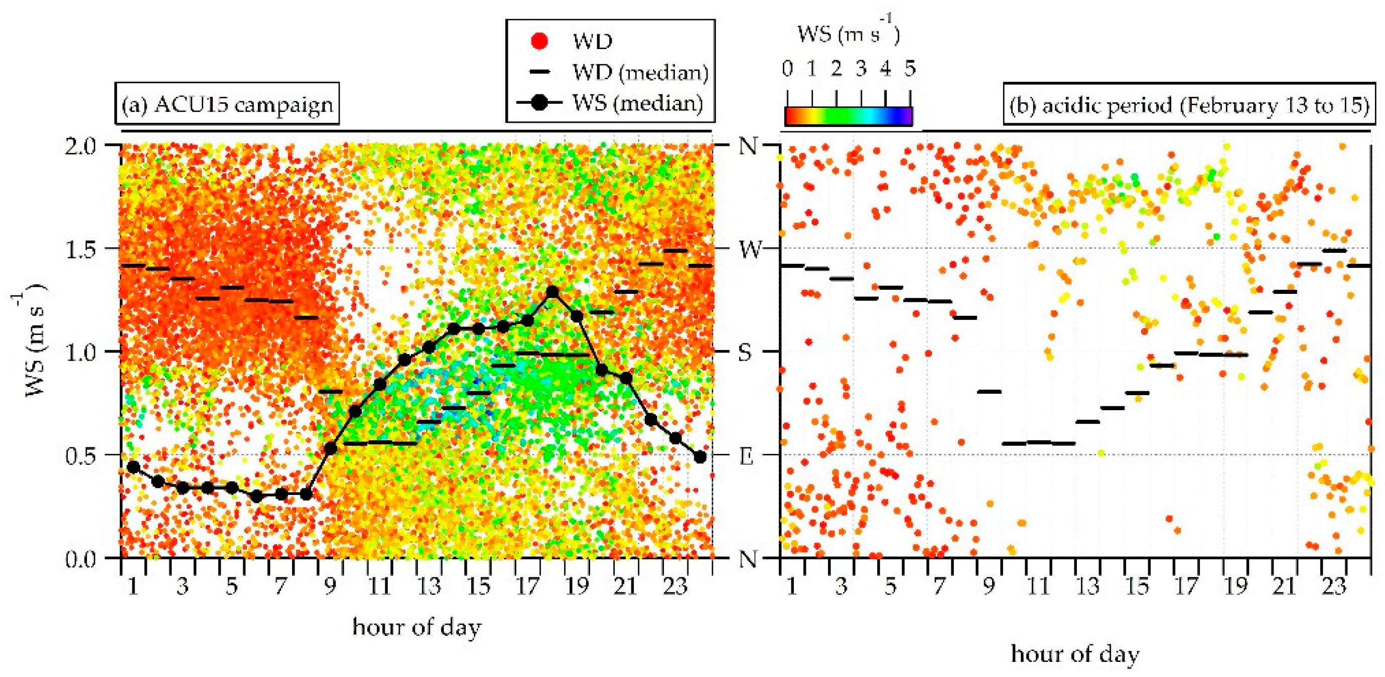
During the first acidic period, the meteorological conditions (wind speed and direction, temperature, and relative humidity) were different from the rest of the campaign: the temperature was lower (Tacidic-period = 11.9 °C, Tcampaing-average = 15.2 °C) and the relative humidity higher (RHacidic-period = 57.7%, RHcampaign-average = 46.0%). In general, both conditions promote the acidity of aerosols because a lower temperature shifts the phase equilibrium of nitric acid to the condensed phase, and a higher relative humidity enhances the conversion of SO2 to sulfate [37]. The wind patterns also showed a different behavior than average during the acidic period as shown in Figure 6. Panel a, shows the wind direction (5-min average) as a function of time of day; the median WD and WS during the whole campaign are also shown. In general, there were north-westerly winds during the night, which shifted direction (south-easterly) around 8 a.m., with increased speed. The wind direction in the afternoon was very variable, with a median from the south-east until 9 p.m. However, panel b shows that during the acidic period the afternoon wind came predominantly from the north, with highest wind velocities around 5 p.m. Northerly winds, in general, are expected to transport air from the main sources of SO2 in the metropolitan area [9,34]. Although the SO2 concentration during the acidic period was relatively high (see Figure 2), there were other periods with higher SO2 concentration with no acidic characteristics. This is an indication that all conditions (northerly winds, low temperatures, and high relative humidity) were responsible for the acidity during the discussed period.
The second period (3 March from 6:20 to 15:24) was very short and the meteorological conditions were not significantly different from the rest of the campaign.
Another explanation for the ion imbalance observed could be the presence of organic nitrates (ON), which would generate nitrate ions in the mass spectrometer, but would not contribute to the acidity of the particles. Unfortunately, the identification of ONs, especially with a unit mass resolution spectrometer such as the ACSM, is difficult because they are expected to occur along with the inorganic nitrate, which generates a large background signal. To date, there is no known unambiguous ion marker to identify the organic nitrates [38]. It is expected that organic nitrates are present in secondary organic aerosol (SOA); however, during the acidic periods described above, the oxygenated organic aerosol (OA, see next section for details) did not correlate with ammonium_miss, while sulfate did. Hence, the effect of the presence of ON on the ion balance might be small, which is consistent with results during MILAGRO, when little indication was found of the presence of a large amount of ON in the atmosphere [13].
3.4. Organic Fraction
The PMF model was used to further investigate the nature of the organic fraction of the aerosol. A solution with three factors was chosen based on the suggestions from Zhang, et al. [39] to evaluate the results of the model. In addition, mass spectra profiles, time series, diurnal cycles, and correlations with other species were analyzed too, as described below.
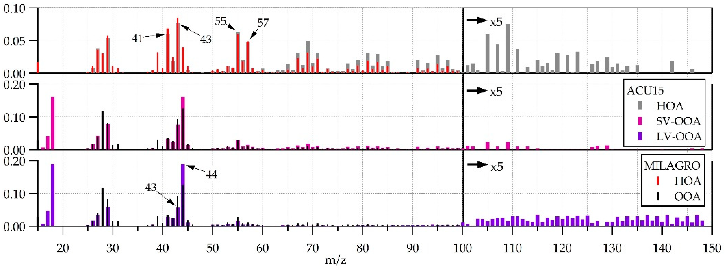
The PMF solution chosen consisted of three factors which were assigned to hydrocarbon-like organic aerosol (HOA), semi-volatile oxygenated organic aerosol (SV-OOA), and low-volatility oxygenated organic aerosol (LV-OOA). Figure 7 shows the mass spectra of the three profiles. The HOA factor is compared to the HOA factor found during MILAGRO, where the ion series CnH+2n+1 and CnH2+2n−1 (which includes m/z 41, 43, 55, 57) are distinguishable. The two OOA factors are compared to the one OOA factor found during MILAGRO, where the ion at m/z 44 (CO2+) is predominant [40].
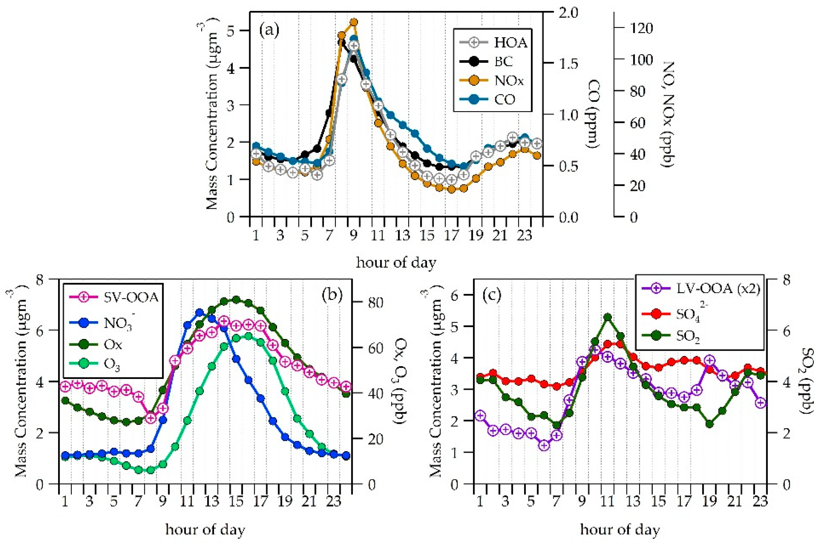
The classification of the organic factors is further justified in Figure 8, by comparing their diurnal profiles to those of other species. The HOA factor, as expected from fresh organic emissions from vehicles, shows a maximum at 9 a.m. together with CO and NOx which is the time at which most activity starts at the university campus. NO and BC seems to peak one hour before, which probably is explained by the public transport station located approximately 300 m from the site, where activities start earlier. On the other hand, the SV-OOA factor has a maximum similar to the “total oxidant” Ox (Ox = O3 + NO2), which is a proxy for the “real” photochemical production of O3 because it takes into account the rapid interconversion between NO2 and O3 [41]. This similarity is indicative of fresh production of secondary organic aerosol. Although the increase of the SV-OOA component starts at the same time as the nitrate, the latter decreases around noon while the organics remain high. This observation is probably related to the relative volatility of both aerosol components: the ammonium nitrate might be more volatile and tend to evaporate faster as the temperature increases during mid-morning. Finally, the LV-OOA has a diurnal cycle very similar to sulfate and SO2. In the figure, the acidic period was not included in the calculation of the hourly averages. As explained above, the SO2 is primarily emitted in the northern part of the city and the sulfate is known to have a regional character in the MCMA [18]; hence, the LV-OOA probably corresponds to an aged organic aerosol.
The PMF model was not able to resolve a biomass burning organic aerosol factor (BBOA, with a relatively large contribution of the ion ate m/z 60), which was found during MILAGRO using high resolution mass spectra, probably due to the low resolution in time and m/z of the ACSM. Figure 9 shows the time series of the ions at m/z 60, which had two periods with large plumes at the end of February and the beginning of April. Plumes of HOA and SV-OOA were also observed during those periods.
The time series, and diurnal cycles of the PMF organic factors are shown in Figure 10. The percent composition of the OA is also shown in the figure. The LV-OOA is the largest fraction of the OOA (63%), followed by HOA (22%), and SV-OOA is the smallest fraction (15%). During MILAGRO the HOA comprised a larger fraction (29%) [13], which is an indication of the impact of the primary sources, which are larger in the north of the city [34]. The OOA contribution to the organic mass (SV-OOA + LV-OOA = 78%) is larger during ACU15 than during MILAGRO (OOA 46%), even including BBOA (16%), due to the importance of the LV-OOA.
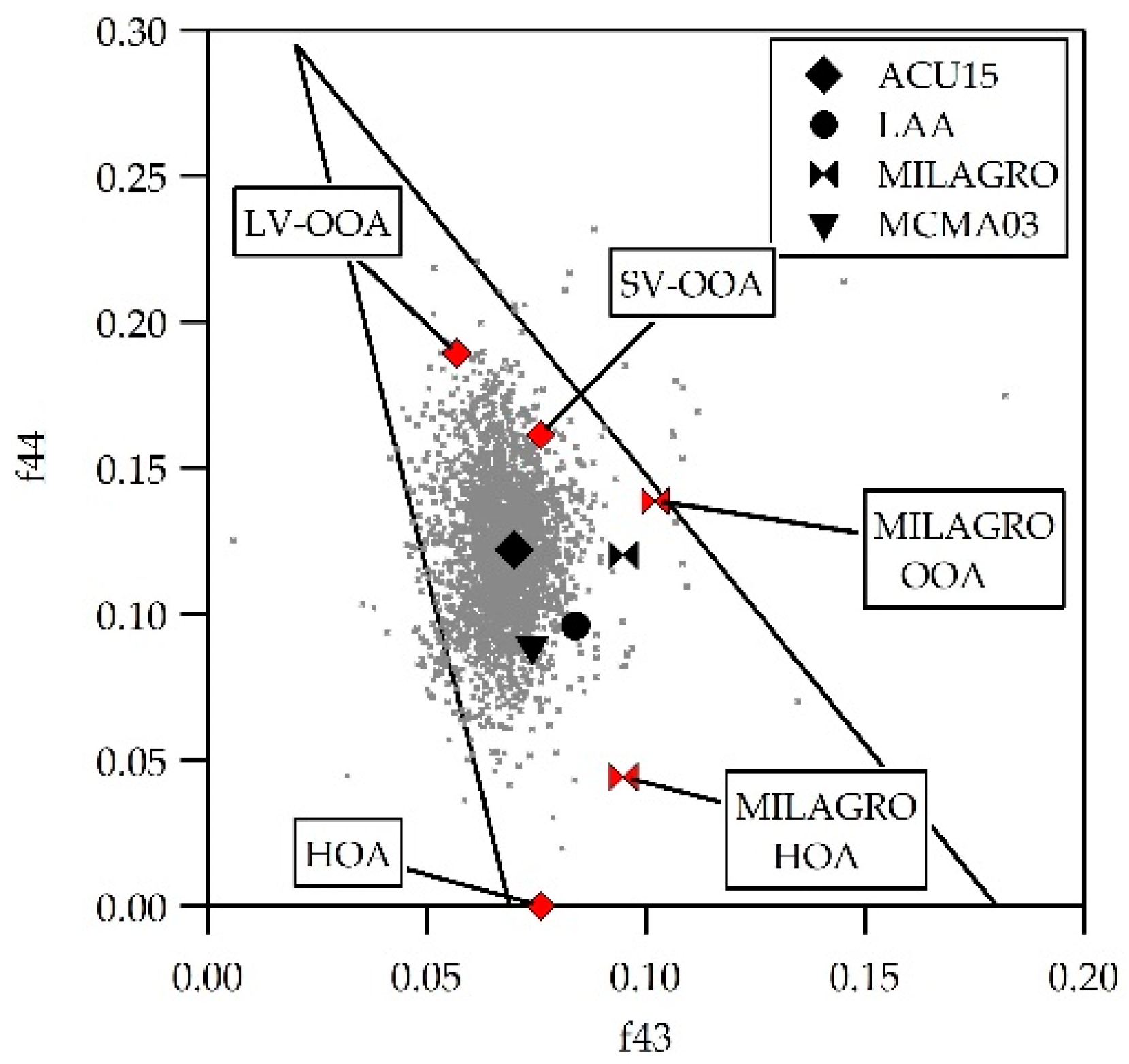
The triangle plot described by Ng et al. [40] can be of further help to classify the organic components described above. The analysis uses ions m/z 44 and m/z 43 as a diagnostic for the aging of the OA. By plotting f44 vs. f43 (fm/z is the fraction of the ion’s signal to the total signal of the component), it is easy to see that the OOA components tend to become similar to fulvic acid and HULIS (humic-like substances). In Figure 11, f44 data during ACU15 are plotted vs. f43. The average f44 vs. f43 for all the AMS campaigns is also shown. The lines in the figure are added as guidelines and define region where ambient OOA data fall. In this diagram, the closer the data are to the intersection of the lines, the more oxidized is the organic component, i.e., it is more aged. Hence, the position that corresponds to the ACU15 indicates more aged aerosol than the observed previously, which is also consistent with a larger fraction of sulfate as previously discussed. In addition, the LV-OOA is also more oxidized than SV-OOA, which is consistent with the classification.
4. Conclusions
The chemical composition of NR-PM1 in a site south of Mexico City was reported for the first time with a high time resolution. The mass concentration in the site was lower than reported in previous campaigns that took place north and east of the city, using similar equipment. This difference in total NR-PM1 mass concentration might be explained by the natural variability of the atmospheric conditions, as well as the different sources impacting each site.
In general, the daily variability of all the aerosol components were as expected from previous campaigns. However, regarding the chemical composition of the aerosol, we found significant differences which indicate that the aerosol is more aged in the south than the north and east of the MCMA. During ACU15, half of the NR-PM1 mass consisted of organic matter, of which almost three quarters correspond to a low volatile oxygenated organic aerosol. In addition, one quarter of the total NR-PM1 mass corresponded to sulfate, which was significantly higher than what was reported in other sites. These observations are indicative of a more processed aerosol, which is consistent with the distribution of the PM sources and precursors within the city, as well as with the meteorological patterns that usually occur in the metropolitan area.
The results presented in this study suggest that the aerosol composition across Mexico City, as well as the processes associated with them, are more heterogenous than previous studies (which occurred in specific sites and time of the year) had suggested. Hence, it is important to have more studies on larger time and space scales, in order to understand the aerosol chemistry in the city under different meteorological conditions, and in sites with different characteristics.
Supplementary Materials
The following are available online at https://www.mdpi.com/2073-4433/9/6/232/s1, Figure S1: Time series and scatter plots of PM mass concentration from co-located instruments, Figure S2: Time series of PM2.5 monthly concentration at three sites of the Mexico City’s Atmospheric Monitoring Network.
Author Contributions
O.P. and T.C. designed and coordinated the ACU15 campaign; D.S. and H.A.-O. oversaw the ACSM operation, and the data analysis; D.S. wrote the paper.
Funding
This research was funded by Dirección General de Asuntos del Personal Académico, Universidad Nacional Autónoma de México: PAPIIT IN113416.
Acknowledgments
This research was supported by program UNAM-DGAPA-PAPIIT IN113416. We thank María Isabel Saavedra Rosado for technical help during the campaign.
Conflicts of Interest
The authors declare no conflict of interest. The founding sponsors had no role in the design of the study; in the collection, analyses, or interpretation of data; in the writing of the manuscript; and in the decision to publish the results.
References
- Secretaría del Medio Ambiente de la Ciudad de México (SEDEMA). Calidad del Aire en la Ciudad de México Informe 2014; Secretaría del Medio Ambiente de la Ciudad de México: Ciudad de México, Mexico, 2015.
- Molina, L.; Molina, M. Air Quality in the Mexico Megacity. An Integrated Assessment; Springer: Dordrecht, The Netherlands, 2002; Volume 2. [Google Scholar]
- Secretaría del Medio Ambiente de la Ciudad de México (SEDEMA). Calidad del Aire en la Ciudad de México Informe 2015; Secretaría del Medio Ambiente de la Ciudad de México: Ciudad de México, Mexico, 2016.
- Secretaría del Medio Ambiente de la Ciudad de México (SEDEMA). Calidad del Aire en la Ciudad de México Informe 2016; Secretaría del Medio Ambiente de la Ciudad de México: Ciudad de México, Mexico, 2017.
- Secretaría del Medio Ambiente del Gobierno del Distrito Federal (SMADF). Calidad del Aire en la Ciudad de México Informe 2011; Secretaría del Medio Ambiente del Gobierno del Distrito Federal: Mexico City, Mexico, 2012.
- Secretaría del Medio Ambiente del Gobierno del Distrito Federal (SMADF). Calidad del Aire en la Ciudad de México Informe 2013; Secretaría del Medio Ambiente del Gobierno del Distrito Federal: Mexico City, Mexico, 2014.
- Instituto Nacional de Estadística y Geografía (INEGI). Encuesta Origen Destino en Hogares de la Zona Metropolitana del Valle de México 2017; Instituto Nacional de Estadística y Geografía: Aguascalientes, Mexico, 2018.
- Carreón-Sierra, S.; Salcido, A.; Castro, T.; Celada-Murillo, A.-T. Cluster analysis of the wind events and seasonal wind circulation patterns in the mexico city region. Atmosphere 2015, 6, 1006–1031. [Google Scholar] [CrossRef]
- De Foy, B.; Krotkov, N.A.; Bei, N.; Herndon, S.C.; Huey, L.G.; Martínez, A.P.; Ruiz-Suárez, L.G.; Wood, E.C.; Zavala, M.; Molina, L.T. Hit from both sides: Tracking industrial and volcanic plumes in Mexico city with surface measurements and OMI SO2 retrievals during the milagro field campaign. Atmos. Chem. Phys. 2009, 9, 9599–9617. [Google Scholar] [CrossRef]
- Molina, L.T.; Kolb, C.E.; de Foy, B.; Lamb, B.K.; Brune, W.H.; Jimenez, J.L.; Ramos-Villegas, R.; Sarmiento, J.; Paramo-Figueroa, V.H.; Cardenas, B.; et al. Air quality in north america’s most populous city—Overview of the MCMA-2003 campaign. Atmos. Chem. Phys. 2007, 7, 2447–2473. [Google Scholar] [CrossRef]
- Molina, L.T.; Madronich, S.; Gaffney, J.S.; Apel, E.; de Foy, B.; Fast, J.; Ferrare, R.; Herndon, S.; Jimenez, J.L.; Lamb, B.; et al. An overview of the milagro 2006 campaign: Mexico city emissions and their transport and transformation. Atmos. Chem. Phys. 2010, 10, 8697–8760. [Google Scholar] [CrossRef] [Green Version]
- Aiken, A.C.; de Foy, B.; Wiedinmyer, C.; DeCarlo, P.F.; Ulbrich, I.M.; Wehrli, M.N.; Szidat, S.; Prevot, A.S.H.; Noda, J.; Wacker, L.; et al. Mexico city aerosol analysis during milagro using high resolution aerosol mass spectrometry at the urban supersite (T0)—Part 2: Analysis of the biomass burning contribution and the non-fossil carbon fraction. Atmos. Chem. Phys. 2010, 10, 5315–5341. [Google Scholar] [CrossRef] [Green Version]
- Aiken, A.C.; Salcedo, D.; Cubison, M.J.; Huffman, J.A.; DeCarlo, P.F.; Ulbrich, I.M.; Docherty, K.S.; Sueper, D.; Kimmel, J.R.; Worsnop, D.R.; et al. Mexico city aerosol analysis during milagro using high resolution aerosol mass spectrometry at the urban supersite (T0)—Part 1: Fine particle composition and organic source apportionment. Atmos. Chem. Phys. 2009, 9, 6633–6653. [Google Scholar] [CrossRef]
- Baumgardner, D.; Grutter, M.; Allan, J.; Ochoa, C.; Rappenglueck, B.; Russell, L.M.; Arnott, P. Physical and chemical properties of the regional mixed layer of mexico’s megapolis. Atmos. Chem. Phys. 2009, 9, 5711–5727. [Google Scholar] [CrossRef]
- DeCarlo, P.; Dunlea, E.; Kimmel, J.; Aiken, A.; Sueper, D.; Crounse, J.; Wennberg, P.; Emmons, L.; Shinozuka, Y.; Clarke, A. Fast airborne aerosol size and chemistry measurements above Mexico city and central Mexico during the milagro campaign. Atmos. Chem. Phys. 2008, 8, 4027–4048. [Google Scholar] [CrossRef]
- Dzepina, K.; Arey, J.; Marr, L.C.; Worsnop, D.R.; Salcedo, D.; Zhang, Q.; Onasch, T.B.; Molina, L.T.; Molina, M.J.; Jimenez, J.L. Detection of particle-phase polycyclic aromatic hydrocarbons in Mexico city using an aerosol mass spectrometer. Int. J. Mass Spectrom. 2007, 263, 152–170. [Google Scholar] [CrossRef]
- Salcedo, D.; Onasch, T.B.; Aiken, A.C.; Williams, L.R.; de Foy, B.; Cubison, M.J.; Worsnop, D.R.; Molina, L.T.; Jimenez, J.L. Determination of particulate lead using aerosol mass spectrometry: Milagro/MCMA-2006 observations. Atmos. Chem. Phys. 2010, 10, 5371–5389. [Google Scholar] [CrossRef] [Green Version]
- Salcedo, D.; Onasch, T.B.; Dzepina, K.; Canagaratna, M.R.; Zhang, Q.; Huffman, J.A.; DeCarlo, P.F.; Jayne, J.T.; Mortimer, P.; Worsnop, D.R.; et al. Characterization of ambient aerosols in Mexico city during the MCMA-2003 campaign with aerosol mass spectrometry: Results from the cenica supersite. Atmos. Chem. Phys. 2006, 6, 925–946. [Google Scholar] [CrossRef]
- Guerrero, F.; Álvarez-Ospina, H.; Retama, A.; López-Medina, A.; Castro, T.; Salcedo, D. Seasonal changes in the PM1 chemical composition north of Mexico city. Atmósfera 2017, 30, 243–273. [Google Scholar] [CrossRef]
- Ng, N.L.; Herndon, S.C.; Trimborn, A.; Canagaratna, M.R.; Croteau, P.L.; Onasch, T.B.; Sueper, D.; Worsnop, D.R.; Zhang, Q.; Sun, Y.L.; et al. An aerosol chemical speciation monitor (ACSM) for routine monitoring of the composition and mass concentrations of ambient aerosol. Aerosol Sci. Technol. 2011, 45, 780–794. [Google Scholar] [CrossRef]
- Retama, A.; Baumgardner, D.; Raga, G.B.; McMeeking, G.R.; Walker, J.W. Seasonal and diurnal trends in black carbon properties and co-pollutants in Mexico city. Atmos. Chem. Phys. 2015, 15, 9693–9709. [Google Scholar] [CrossRef]
- Von der Weiden, S.L.; Drewnick, F.; Borrmann, S. Particle loss calculator—A new software tool for the assessment of the performance of aerosol inlet systems. Atmos. Meas. Tech. 2009, 2, 479–494. [Google Scholar] [CrossRef]
- Canagaratna, M.R.; Jayne, J.T.; Jimenez, J.L.; Allan, J.D.; Alfarra, M.R.; Zhang, Q.; Onasch, T.B.; Drewnick, F.; Coe, H.; Middlebrook, A.; et al. Chemical and microphysical characterization of ambient aerosols with the aerodyne aerosol mass spectrometer. Mass Spectrom. Rev. 2007, 26, 185–222. [Google Scholar] [CrossRef] [PubMed]
- Paatero, P.; Tapper, U. Positive matrix factorization: A non-negative factor model with optimal utilization of error estimates of data values. Environmetrics 1994, 5, 111–126. [Google Scholar] [CrossRef]
- Ulbrich, I.M.; Canagaratna, M.R.; Zhang, Q.; Worsnop, D.R.; Jimenez, J.L. Interpretation of organic components from positive matrix factorization of aerosol mass spectrometric data. Atmos. Chem. Phys. 2009, 9, 2891–2918. [Google Scholar] [CrossRef]
- Wavemetrics. Igor Pro v6.36 User's Guide; Wavemetrics Inc.: Lake Oswego, OR, USA, 2014. [Google Scholar]
- Patrick Arnott, W.; Moosmüller, H.; Fred Rogers, C.; Jin, T.; Bruch, R. Photoacoustic spectrometer for measuring light absorption by aerosol: Instrument description. Atmos. Environ. 1999, 33, 2845–2852. [Google Scholar] [CrossRef]
- Wang, Q.; Huang, R.J.; Cao, J.; Han, Y.; Wang, G.; Li, G.; Wang, Y.; Dai, W.; Zhang, R.; Zhou, Y. Mixing state of black carbon aerosol in a heavily polluted urban area of China: Implications for light absorption enhancement. Aerosol Sci. Technol. 2014, 48, 689–697. [Google Scholar] [CrossRef]
- Bond, T.C.; Habib, G.; Bergstrom, R.W. Limitations in the enhancement of visible light absorption due to mixing state. J. Geophys. Res. Atmos. 2006, 111. [Google Scholar] [CrossRef] [Green Version]
- He, C.; Liou, K.N.; Takano, Y.; Zhang, R.; Levy Zamora, M.; Yang, P.; Li, Q.; Leung, L.R. Variation of the radiative properties during black carbon aging: Theoretical and experimental intercomparison. Atmos. Chem. Phys. 2015, 15, 11967–11980. [Google Scholar] [CrossRef]
- Pavia-Hernández, R. Eficiencia de Absorción de Masa de Carbono Elemental y Propiedades Ópticas de Partículas Atmosféricas PM2.5; Universidad Nacional Autónoma de México (UNAM): Mexico City, Mexico, 2016. [Google Scholar]
- SIMAT. Available online: http://www.aire.cdmx.gob.mx (accessed on 24 April 2018).
- Querol, X.; Pey, J.; Minguillón, M.C.; Pérez, N.; Alastuey, A.; Viana, M.; Moreno, T.; Bernabé, R.M.; Blanco, S.; Cárdenas, B.; et al. Pm speciation and sources in Mexico during the milagro-2006 campaign. Atmos. Chem. Phys. 2008, 8, 111–128. [Google Scholar] [CrossRef]
- Secretaría del Medio Ambiente de la Ciudad de México (SEDEMA). Inventario de Emisiones de la CDMX 2014. Contaminates Criterio, Tóxicos y de Efecto Invernadero; Secretaría del Medio Ambiente de la Ciudad de México: Ciudad de México, Mexico, 2016.
- De Foy, B.; Caetano, E.; Magaña, V.; Zitácuaro, A.; Cárdenas, B.; Retama, A.; Ramos, R.; Molina, L.T.; Molina, M.J. Mexico city basin wind circulation during the MCMA-2003 field campaign. Atmos. Chem. Phys. 2005, 5, 2267–2288. [Google Scholar] [CrossRef]
- De Foy, B.; Fast, J.D.; Paech, S.J.; Phillips, D.; Walters, J.T.; Coulter, R.L.; Martin, T.J.; Pekour, M.S.; Shaw, W.J.; Kastendeuch, P.P.; et al. Basin-scale wind transport during the milagro field campaign and comparison to climatology using cluster analysis. Atmos. Chem. Phys. 2008, 8, 1209–1224. [Google Scholar] [CrossRef]
- Seinfeld, J.H.; Pandis, S.N. Atmospheric Chemistry and Physics: From Air Pollution to Climate Change; John Wiley & Sons: Hoboken, NJ, USA, 2012. [Google Scholar]
- Rollins, A.W.; Fry, J.L.; Hunter, J.F.; Kroll, J.H.; Worsnop, D.R.; Singaram, S.W.; Cohen, R.C. Elemental analysis of aerosol organic nitrates with electron ionization high-resolution mass spectrometry. Atmos. Meas. Tech. 2010, 3, 301–310. [Google Scholar] [CrossRef] [Green Version]
- Zhang, Q.; Jimenez, J.L.; Canagaratna, M.R.; Ulbrich, I.M.; Ng, N.L.; Worsnop, D.R.; Sun, Y. Understanding atmospheric organic aerosols via factor analysis of aerosol mass spectrometry: A review. Anal. Bioanal. Chem. 2011, 401, 3045–3067. [Google Scholar] [CrossRef] [PubMed]
- Ng, N.L.; Canagaratna, M.R.; Zhang, Q.; Jimenez, J.L.; Tian, J.; Ulbrich, I.M.; Kroll, J.H.; Docherty, K.S.; Chhabra, P.S.; Bahreini, R.; et al. Organic aerosol components observed in northern hemispheric datasets from aerosol mass spectrometry. Atmos. Chem. Phys. 2010, 10, 4625–4641. [Google Scholar] [CrossRef]
- Lu, K.; Zhang, Y.; Su, H.; Brauers, T.; Chou Charles, C.; Hofzumahaus, A.; Liu Shaw, C.; Kita, K.; Kondo, Y.; Shao, M.; et al. Oxidant (O3 + NO2) production processes and formation regimes in beijing. J. Geophys. Res. Atmos. 2010, 115. [Google Scholar] [CrossRef]
Figure 1.
Map of the Mexico City Metropolitan Area, showing the sites mentioned in the text (red stars). Thick black lines represent state boundaries, and thin grey contour lines represent topographical features. Urban areas are colored in grey. LAA: Laboratorio de Análisis Ambiental; CCA: Centro de Ciencias de la Atmósfera.
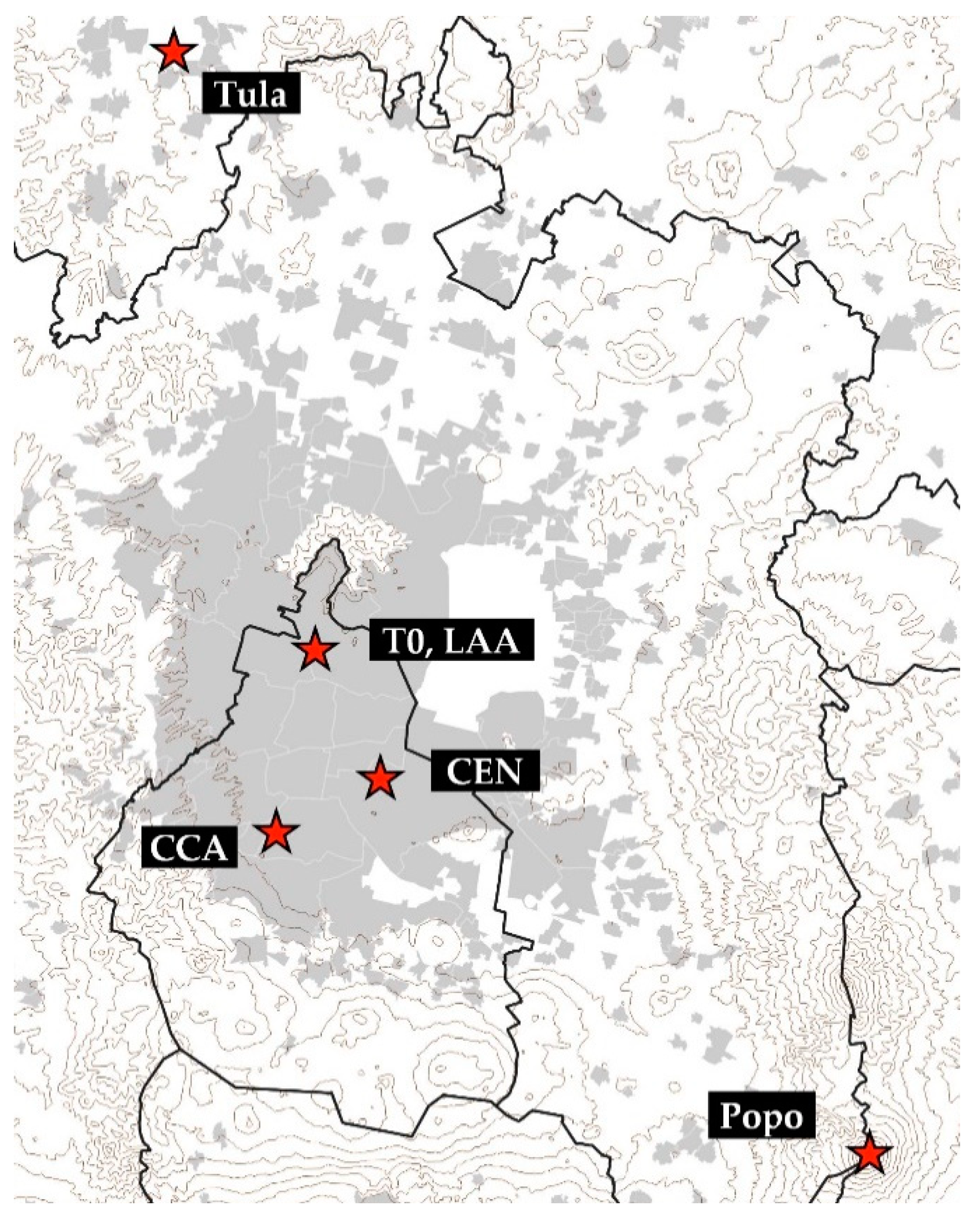
Figure 2.
Time series of the mass concentration and fraction of the non-refractory submicron particulate matter (NR-PM1) components (organics, sulfate, nitrate, ammonium, and chloride), meteorological variables (temperature (T), relative humidity (RH), wind speed (WS) and direction (WD), and rain), black carbon (BC), and other pollutants (CO, SO2, O3, and NOx) during ACU15. The gray area highlights the acidic periods mentioned in Section 3.3. ACU15: Aerosoles en Ciudad Universitaria 2015.
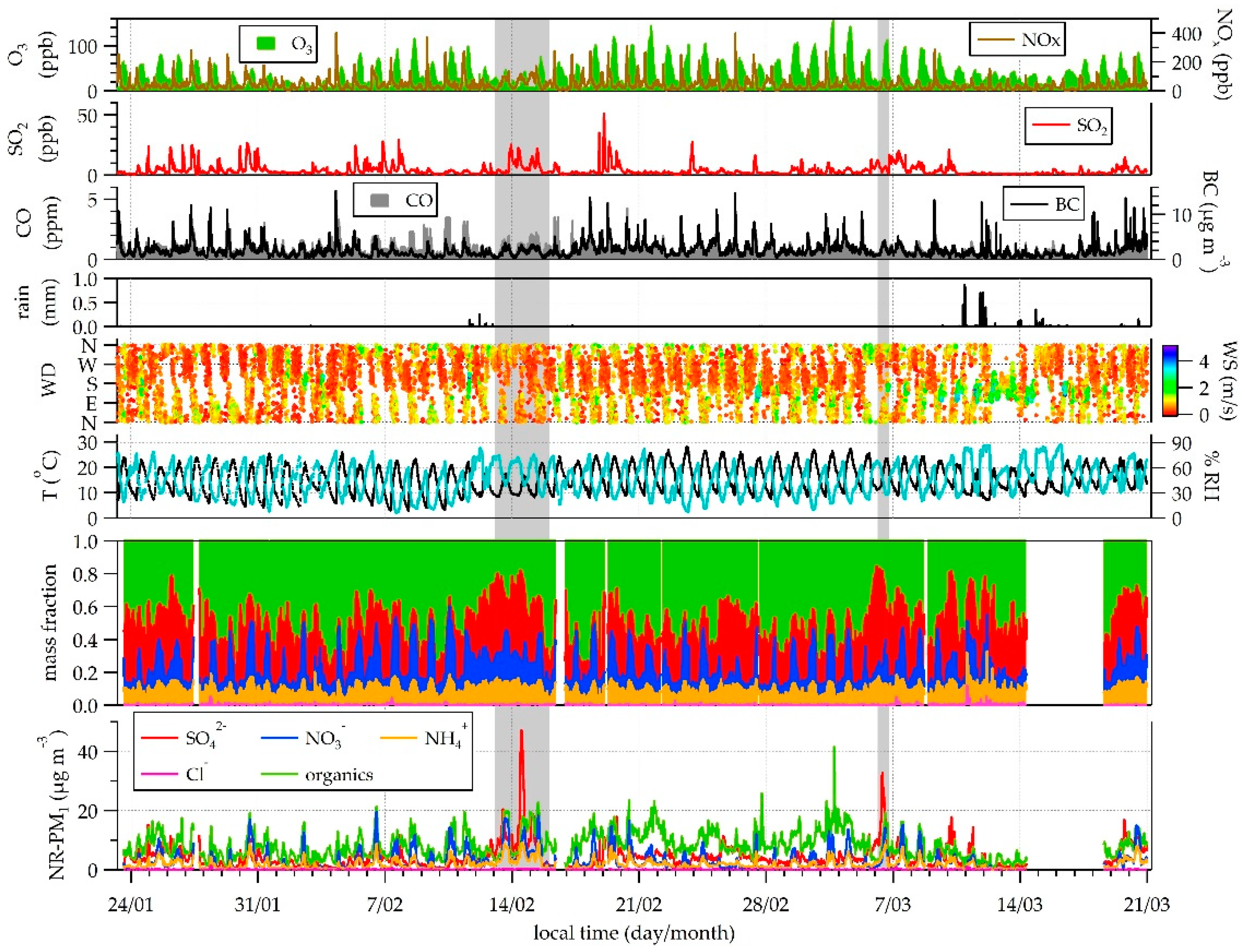
Figure 3.
Average mass fraction diurnal profile and average percent composition of NR-PM1 as determined by the Aerosol Chemical Speciation Monitor (ACSM) during ACU15.
Figure 3.
Average mass fraction diurnal profile and average percent composition of NR-PM1 as determined by the Aerosol Chemical Speciation Monitor (ACSM) during ACU15.
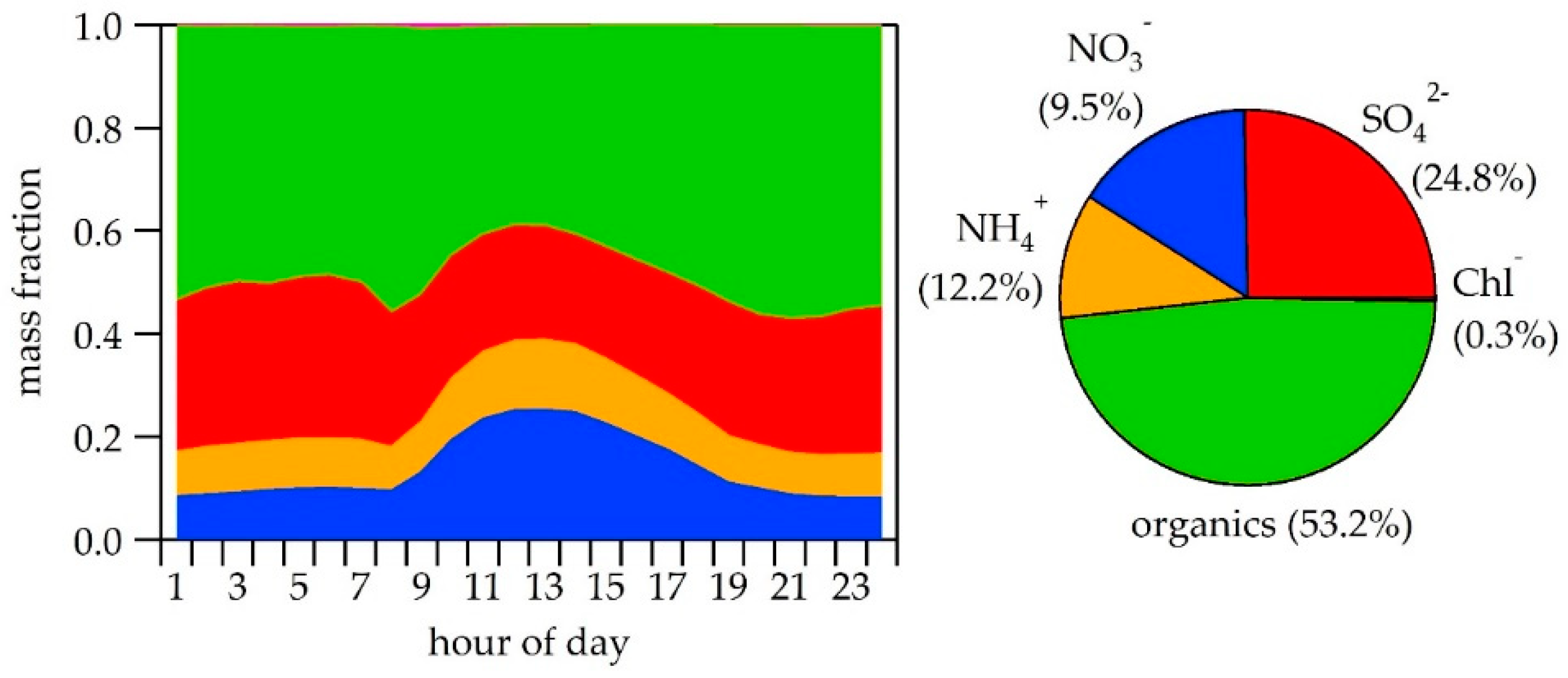
Figure 4.
Average diurnal profiles of the mass concentration of the total NR-PM1 and its component during ACU15 and previous studies in Mexico City involving an AMS [13,18,19]. AMS: Aerosol Mass Spectrometer.
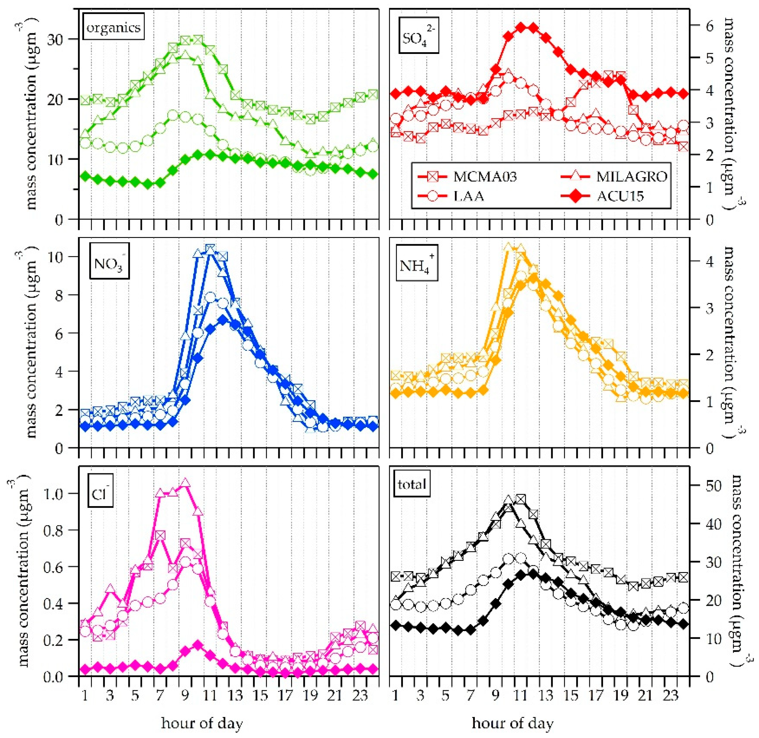
Figure 5.
(a) Scatter plot of the predicted ammonium assuming neutrality (ammonium_pred) vs. the measured ammonium. (b) Time series of the extra ammonium needed to neutralize the aerosol (ammonium_mis). Data points with ammonium_mis larger than the average plus one standard deviation are colored in black for visualization purposes.
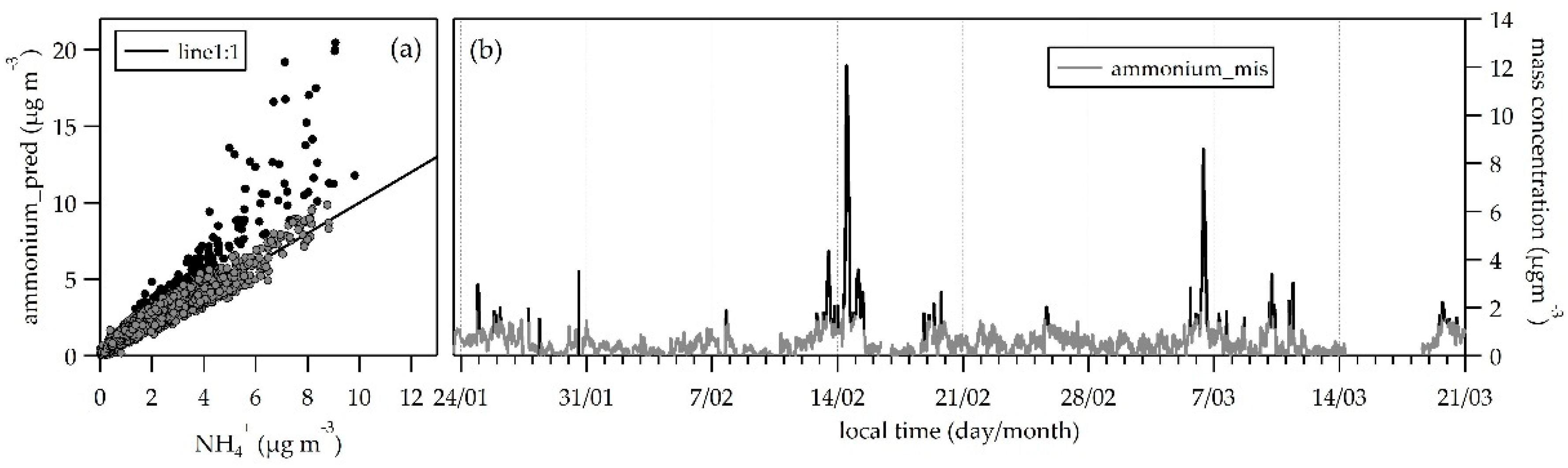
Figure 6.
Wind speed (WS) and wind direction (WD) vs. hour of the day. Black circles represent the median WS during the campaign, and black horizontal bars in both panels represent the median WD during the campaign. Colored small circles, are 15 min wind data for the whole campaign (a) and during the first acidic period (b).

Figure 7.
Mass spectra of the Positive Matrix Factorization (PMF) organic factors during ACU15 and MILAGRO (Megacity Initiative: Local And Global Research Observations) [13]. HOA: hydrocarbon-like organic aerosol; SV-OOA: semi-volatile oxygenated organic aerosol; LV-OOA: low-volatility oxygenated organic aerosol.

Figure 8.
Average diurnal profiles of the mass concentration of the PMF-AMS organic factors during ACU15. Each factor is compared with other atmospheric species as markers of primary emissions (a), photochemistry (b), and regional transport (c).
Figure 8.
Average diurnal profiles of the mass concentration of the PMF-AMS organic factors during ACU15. Each factor is compared with other atmospheric species as markers of primary emissions (a), photochemistry (b), and regional transport (c).

Figure 9.
(a) Time series of the signal of ion m/z 60 during ACU15. (b) Times series of the signal of ion m/z 60, organics in NR-PM1, and hydrocarbon-like organic aerosol (HOA) and semi-volatile oxygenated organic aerosol (SV-OOA) PMF factors from 27 February to 5 March. All signals are scaled arbitrarily.
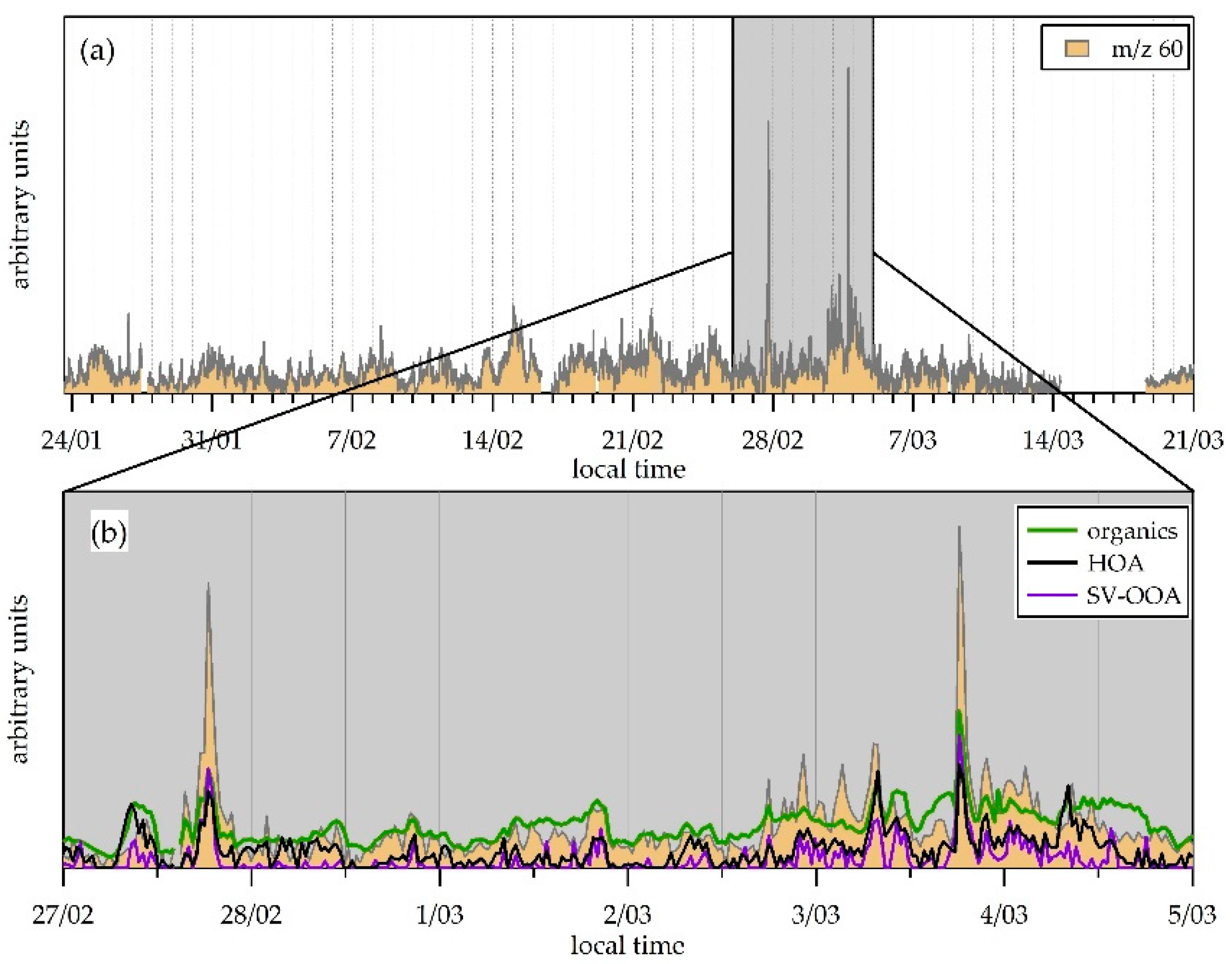
Figure 10.
Time series, diurnal profiles, and percent of total organic mass of PMF organic factors.
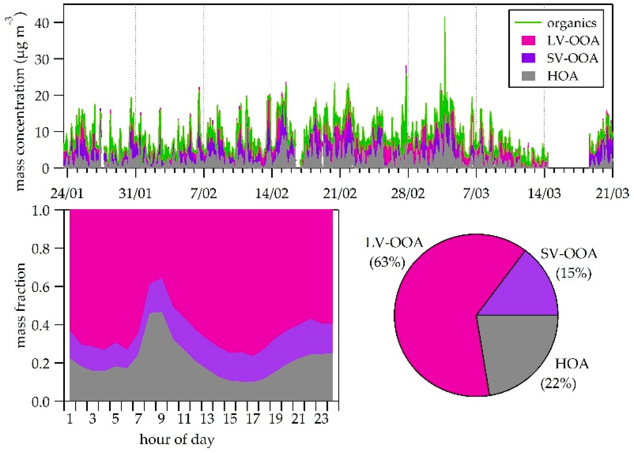
Figure 11.
f44 vs. f43 of the Organics mass spectra. Grey points correspond to all data points during ACU15. Black symbols correspond to average f44 vs. f43 during the AMS campaigns [13,18,19]. Red symbols correspond to the PMF OOA factors during ACU15 and MILAGRO [13].


Table 1.
Summary of PM data during ACU15 and previous studies in Mexico City involving an AMS.
| ACU15 (CCA) | LAA [19] | MILAGRO (T0) [13] | MCMA03 (CEN) [18] | ||||||
|---|---|---|---|---|---|---|---|---|---|
| 21 January–23 March 2015 | 13 November 2013–30 April 2014 | 1 March–4 April 2006 | 31 March–4 May 2003 | ||||||
| (µg m−3) | % | (µg m−3) | % | (µg m−3) | % | (µg m−3) | % | ||
| NR-PM1 | organics | 8.1 | 53.2 | 12.0 | 59.3 | 17.3 | 64.6 | 21.6 | 69.9 |
| sulfate | 4.3 | 24.8 | 3.2 | 16.1 | 3.6 | 13.4 | 3.1 | 10.1 | |
| nitrate | 2.7 | 12.2 | 2.9 | 14.4 | 3.5 | 13.1 | 3.7 | 11.9 | |
| ammonium | 1.8 | 9.5 | 1.8 | 9.0 | 2.0 | 7.7 | 2.2 | 7.0 | |
| chloride | 0.05 | 0.3 | 0.2 | 1.2 | 0.4 | 1.5 | 0.3 | 1.0 | |
| ACSM total | 16.9 | 20.2 | 26.8 | 30.9 | |||||
| BC (PM2.5) | 2.1a | 3.03 a | 4.2 *,c | 3.4 *,c | |||||
| soil (PM2.5) | 1.7 § | 2.1 | |||||||
| metals (PM2.5) | 1.0 | ||||||||
| PM2.5 | 17.5 b, 16.1 c | 37.0 b | 40.0 d [33] | 35.7 b, 40.0 e | |||||
| PM1 | 27.8 b | 33.0 d [33] | |||||||
* PM2.0; § PM1; a PAX (Photoacoustic Extinctiometer); b Tapered element oscillating microbalance (TEOM); c Nephelometer; d Optical particle counter (OPC); e Dusttrak. PM: particulate matter; ACU15: Aerosoles en Ciudad Universitaria 2015; AMS: Aerosol Mass Spectrometer; CCA: Centro de Ciencias de la Atmósfera; LAA: Laboratorio de Análisis Ambiental; MCMA: Mexico City Metropolitan Area; MILAGRO: Megacity Initiative: Local And Global Research Observations; NR-PM1: non-refractory submicron particulate matter; ACSM: Aerosol Chemical Speciation Monitor; BC: black carbon.
© 2018 by the authors. Licensee MDPI, Basel, Switzerland. This article is an open access article distributed under the terms and conditions of the Creative Commons Attribution (CC BY) license (http://creativecommons.org/licenses/by/4.0/).
Share and Cite
MDPI and ACS Style
Salcedo, D.; Alvarez-Ospina, H.; Peralta, O.; Castro, T. PM1 Chemical Characterization during the ACU15 Campaign, South of Mexico City. Atmosphere 2018, 9, 232. https://doi.org/10.3390/atmos9060232
AMA Style
Salcedo D, Alvarez-Ospina H, Peralta O, Castro T. PM1 Chemical Characterization during the ACU15 Campaign, South of Mexico City. Atmosphere. 2018; 9(6):232. https://doi.org/10.3390/atmos9060232
Chicago/Turabian StyleSalcedo, Dara, Harry Alvarez-Ospina, Oscar Peralta, and Telma Castro. 2018. "PM1 Chemical Characterization during the ACU15 Campaign, South of Mexico City" Atmosphere 9, no. 6: 232. https://doi.org/10.3390/atmos9060232
Note that from the first issue of 2016, this journal uses article numbers instead of page numbers. See further details here.