Application of Artificial Neural Networks in the Prediction of PM10 Levels in the Winter Months: A Case Study in the Tricity Agglomeration, Poland

Department of Meteorology and Landscape Architecture, West Pomeranian University of Technology in Szczecin, Papieża Pawła VI St 3A, 71-459 Szczecin, Poland
Atmosphere 2018, 9(6), 203; https://doi.org/10.3390/atmos9060203
Submission received: 21 March 2018
/
Revised: 1 May 2018
/
Accepted: 17 May 2018
/
Published: 23 May 2018
(This article belongs to the Section Air Quality)
Abstract
:Poor urban air quality due to high concentrations of particulate matter (PM) remains a major public health problem worldwide. Therefore, research efforts are being made to forecast ambient PM concentrations. In this study, artificial neural networks (ANNs) were employed to generate models forecasting hourly PM10 concentrations 1–6 h ahead, involving 3 measurement locations in the Tricity Agglomeration, Poland. In Poland, the majority of high PM concentration cases occurs in winter due to coal combustion being the main energy carrier. For this reason, the present study covers only the periods of the winter calendar (December, January, February) in the period 2002/2003–2016/2017. Inputs to the models were the values of hourly PM10 concentrations and meteorological factors such as air temperature, relative humidity, air pressure, and wind speed. The results of the neural network models were satisfactory and the values of the coefficient of determination (R2) for the independent test set for three sites ranged from 0.452 to 0.848. The values of the index of agreement (IA) were from 0.693 to 0.957, the fractional mean bias (FB) values were 0 or close to 0 and the root mean square error (RMSE) values varied from 8.80 to 23.56. It is concluded that ANNs have been proven to be effective in the prediction of air pollution levels based on the measured air monitoring data.
1. Introduction
Particle pollution, also known as particulate matter (PM) or particulates, is a complex mixture of different chemical components including water-soluble ions, trace metals, and organic compounds that emerge from a wide range of natural and anthropogenic sources [1,2,3,4]. Generally, two fractions of particulate matter are distinguished: PM10 which is less than 10 µm in particle diameter and PM2.5 which is less than 2.5 µm in diameter. The two fractions differ not only in diameter but also in the time of their formation, their chemical composition, and their half-life time. The structure of the mass size distribution patterns may provide valuable information about the possible PM emission sources. The natural sources significantly affect PM2.5–10 levels, while anthropogenic sources mainly affect the fine fraction [5,6]. In the case of PM originating from industrialized and highly urbanized regions in which nonindustrial combustion (municipal and residential sectors) and traffic are also dominant emission sources, large concentrations of toxic heavy metals are observed [7].
The negative effect of particulate matter pollution on human health, even at relatively low mass concentrations, is widely documented in the literature on the subject [8,9,10,11,12,13,14,15]. According to the latest data, atmospheric PM pollution constitutes the 6th leading risk factor (among 43 ranked), which corresponds to over 3 million deaths worldwide every year [16]. However, contrary to common knowledge and numerous legislative actions (for example, Directive 2008/50/EC in force in the EU) aimed at improving the air quality, pollution from particulate matter still poses the greatest risk to human health. According to the latest report of the European Environmental Agency [17], in 2015, a total of 19% of the EU-28 urban population was exposed to PM10 levels above the daily limit value and approximately 53% was exposed to concentrations exceeding the stricter value for PM10 set by the World Health Organisation (WHO). Moreover, only 2% of the global urban population resides in areas where PM10 concentrations are lower than the values given by the WHO air quality guideline [18]. It is important to note that during smog episodes, the recorded concentrations largely exceed the norm. For example, Kukkonen et al. [19] stated that the recorded maximum 24-h concentrations amounted to 130 μg·m−3 in London (February 2003), approximately 250 μg·m−3 in Oslo (January 2003) and Helsinki (April 2002), and around 400 μg·m−3 in Milan (December 1998). In turn, in the extremely cold January of 2006, the average 24-h PM10 concentration recorded in Kraków exceeded the value of 500 μg·m−3 [20] by three times.
Hence, to take precautions before and during situations in which air quality levels are close to or above the alarm thresholds, researchers have been developing intelligent air pollution forecasting methodologies for public health concerns, mostly based on local modelling works through monitoring data [21,22,23]. Researchers have used statistical modelling techniques and machine learning methods to analyse, engage the proper variables within modelling framework, and, finally, predict the concentrations of particulate matter. The most preferred approaches are multiple linear regression, stepwise regression, artificial neural networks, principal component analysis, and clustering methods [21,22,23,24,25,26,27,28,29]. It should be noted that a number of studies have compared the performance of various modelling approaches to determine the best model for the prediction of PM10 in different locations. Sayegh et al. [25] showed the possibilities of predicting urban PM10 concentrations in the City of Makkah, Saudi Arabia using multiple linear regression, quantile regression model, generalized additive model, and boosted regression trees. Taşpınar and Bozkurt, [26] presented an artificial neural networking model and a multiple linear regression model to forecast the maximum daily PM10 concentrations one day ahead in Düzce, Turkey. In turn, Pires et al. [30] investigated the performance of five linear models (multiple linear regression, principal component regression, independent component regression, quantile regression, and partial least squares regression) to predict the daily mean PM10 concentrations in the Oporto Metropolitan Area.
Many researchers combine numerous statistical methods for the purpose of formulating the most accurate prediction. Voukantsis et al. [31] formulated and employed a novel hybrid scheme in the selection process of input variables for the forecasting models, involving a combination of linear regression and artificial neural networks models for forecasting PM10 and PM2.5 concentrations in Thessaloniki and Helsinki. Ul-Saufie et al. [24] presented the results of daily PM10 forecasting hybrid models obtained from principal component analysis with multiple regression (PCA-MLR) and principal component analysis with feed-forward artificial neural networks (PCA-ANN), comparatively. Similarly, Azid et al. [32] presented the combination of principal component analysis and artificial neural networks allowing for the prediction of the air pollutant index (API) in Malaysia.
Apart from emission, the predictors used in most prognostic models of air quality are weather conditions. The dispersion of pollutants is mainly determined by thermal conditions, air movement dynamics, and the type of circulation or thermal stratification within the atmospheric boundary layer [20,33,34,35,36,37,38,39,40].
Poland wrestles with the problem of excessive particulate matter concentration which is predominantly recorded in urban areas in winter. In Poland, just as in other countries in Central and Eastern Europe, the dependency of the economy on coal is still high. The hard coal and lignite amount to approximately 50, 80, and 77% in the structure of primary energy, electricity, and heat consumption, respectively. It is well recognized that coal combustion is one of the main sources of primary PM and precursor gases emissions [41]. The European Environmental Agency [17] estimated that only in 2012, approximately 44,600 of premature deaths in Poland were attributed to being exposed to PM10. Additionally, two previous winter seasons (D, J, F, 2016/2017 and 2017/2018) in Poland were marked by numerous cases of excessive 24-h PM10 concentrations. In many southern regions of Poland, the Provincial Environmental Protection Inspectorate issued notifications informing on the excessive concentrations both in terms of the need to inform the population (hourly values of 200 μg·m−3), as well as the risk of exceeding the alert levels (hourly values of 300 μg·m−3). In Poland, the concentrations thresholds of PM10 are governed by the Regulation of the Minister of the Environment on 24 August 2012 concerning levels of certain substances in the air. However, it must be emphasized that, in Poland, the thresholds entailing the obligation to inform the population and indicate the risk of exceeding the alert level are, on average, two times (at times even four times) higher than in other European countries.
Therefore, the present paper addresses the topical issue of air quality and aims at presenting the possibility of artificial neural network application to forecast PM10 concentrations in the winter period, 1 to 6 h ahead of time, as conducted in the Tricity Agglomeration on the basis of measurements taken at 3 locations.
2. Materials and Methods
2.1. Research Area
The Tricity Agglomeration is a polycentric metropolitan area located on the coast of Gdańsk Bay in northern Poland. The agglomeration consists of three cities (Gdynia, Sopot, and Gdańsk) with a total area of 414 km2. The main and the most populated city of the agglomeration is Gdańsk. Additionally, Gdańsk and Gdynia are cities which belong to the European Transport Corridor connecting Scandinavia to the rest of Europe. Sopot is a small city providing numerous tourist attractions and is well known for its spas. Sopot is also the most densely populated area of the region. According to data from 31 December 2017, the population of the agglomeration is 747,000 [42]. The basis for the agglomeration’s development and, at the same time, the major source of pollution is the maritime economy—predominantly the shipbuilding industry. Currently, in the agglomeration, there are two ports with numerous container terminals, seven shipyards, and many companies providing services to the aforementioned facilities. The manufacturing-repair character of the ports and shipyards affects the natural environment of the area. Particularly in the area of the shipyards and ports, the air is exposed to pollutants emission, predominantly dust, due to the day-to-day work performed in such facilities (for example, sandblasting, paintwork, or coating) as well as due to transport and loading. Apart from the shipyard industry, a significant share of the pollution is caused by the electrical engineering and petroleum industries. Despite the above, Tricity is characterized by a relatively good air quality regarding the main pollutants [43]. This is due to the favourable location of the agglomeration, as well as due to the fact that in the area of the Tricity agglomeration, the percentage of households connected to the municipal heating network is very high. Furthermore, the percentage of households using gas heating, which greatly limits the pollution that originates from the private use of fossil fuels for domestic heating, is also very high. Additionally, due to a good municipal communication infrastructure, the traffic congestion in the Tricity is relatively small in comparison with other agglomerations in Poland.
2.2. PM10 Data and Meteorological Observation
The study was based on the measurement results of the atmospheric air quality obtained from three monitoring stations located within the area of the Tricity agglomeration and operated by the Foundation Agency of Regional Air Quality Monitoring in Gdańsk (ARMAAG) (Figure 1). The basic materials for the study were the hourly values of PM10 particulate matter concentration, air temperature (AT), relative humidity (RH), atmospheric pressure (PRES), and wind speed (WS), all obtained for the period of the winter calendar (December–February) in the years 2002/2003–2016/2017. The expanded uncertainty of the PM10 measurements in the analysed period amounted to 25%, which is in line with the guidelines of the Directive on Ambient Air Quality and Cleaner Air for Europe [44]. All the stations are defined as urban background stations. Gdańsk Wrzeszcz (λE 21°02′; φN 52°09′) and Gdynia Pogórze (λE 21°02′; φN 52°09′) are located in the built-up and the station in Sopot (λE 21°02′; φN 52°09′) is located in the area of urban allotment gardens.
2.3. Statistical Methods
Artificial neural networks (ANNs) were applied in this research to predict PM10 levels.
Network ANNs are a family of computational machine learning algorithms inspired by the way biological nervous systems process and learn from information [22]. ANNs are one of the favoured techniques in predicting a complex system and can perform any complex function mapping with arbitrarily desired accuracy [23,24]. The neural networks constitute a sophisticated modelling technique which allows for the depiction of the most complex functions. In particular, ANNs are of nonlinear character, which significantly extends the possibilities of application. The basic structure of ANNs is composed of input and output neurons with weights of interconnection placed in different layers and their internal transfer functions. In almost all cases where air pollution models have been developed using ANNs for modelling and forecasting, ANNs have been found to provide more accurate predictions than the traditional linear statistical approaches [22,45,46].
In the end, the models allowing for the prediction of PM10 were created with the following time schedules:
PM10, h+1—the forecast of the PM10 hourly concentration for the next hour
PM10, h+2—the forecast of the PM10 hourly concentration for the next two hours
PM10, h+3—the forecast of the PM10 hourly concentration for the next three hours
PM10, h+4—the forecast of the PM10 hourly concentration for the next four hours
PM10, h+5—the forecast of the PM10 hourly concentration for the next five hours
PM10, h+6—the forecast of the PM10 hourly concentration for the next six hours
To assess the models’ performance between the observed and predicted concentrations of PM10, statistical parameters were used. The following were calculated as performance indicators: index of agreement (IA), fractional mean bias (FB), root mean square error (RMSE), and the coefficient of determination (R2). IA expresses the difference between the predicted and observed values. It is limited to the range 0–1, with high values indicating a good agreement between observations and predictions. FB measures the tendency of a model to over-predict (2 being extreme over-prediction) or under-predict (−2 being extreme under-prediction); the target value for FB is 0. RMSE shows the overall accuracy of the model; smaller values of RMSE denote better model performance. According to Voukantsis [31], RMSE is among the most commonly used indicators when evaluating the performance of ANNs. R2 is considered the basic measure of matching the model to the observed data points; the value range is from 0–1. Its closeness to 1.0 indicates the greater explained variance [23,26,29,31,47]. The indicators used were calculated according to Equations (1)–(4):
where: —total number of measurements at a particular station
—predicted values
—observed values
—mean of the predicted values
—mean of the observed values
—standard deviation of the predicted values
—standard deviation of the observed values
—index of agreement
—fractional mean bias
—root mean square error
—coefficient of determination
All the calculations and statistical analyses were conducted using the STATISTICA Neural Networks software version 12 (Stat Soft, Inc., Tulsa, OK, USA).
3. Results and Discussion
3.1. General Description of PM10 and Meteorology Variables
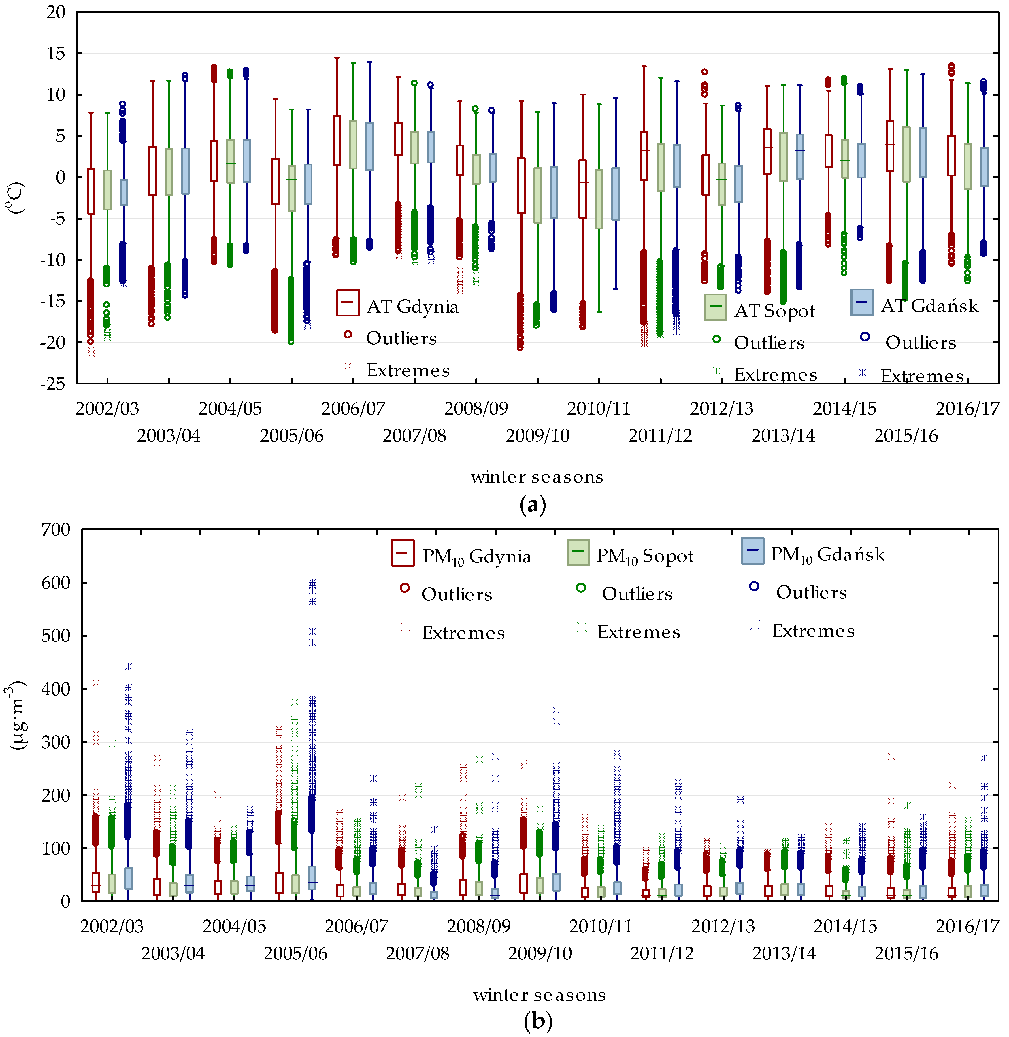
The descriptive statistics of hourly variations of PM10 and meteorological elements used in this study were summarized in Table 1. The temporal variations of the seasonal PM10 and air temperature were illustrated in Figure 2.
The average hourly PM10 concentrations in the 15 analysed winter seasons (2002/2003–2016/2017) (D, J, F) ranged from 26.9 ± 24.9 μg·m−3 in Gdynia, 25.1 ± 23.5 μg·m−3 in Sopot, and 31.0 ± 32.8 μg·m−3 in Gdańsk. For 75% of the hours, the PM10 hourly concentrations were lower than 38 μg·m−3 in Gdańsk, 35 μg·m−3 in Gdynia, and 32 μg·m−3 in Sopot (Table 1). The absolute maximum hourly concentrations recorded in the analysed seasons were 15–20 times higher than the average. In all of the stations, the maximum hourly concentrations exceeded 300 μg·m−3, and in Gdańsk, amounted to approximately 600 μg·m−3 in the winter season of 2005/2006 (Table 1, Figure 2). Such high concentrations were reported in January 2006, when extremely unfavourable meteorological conditions caused by the influence of a Siberian high-pressure system were found to be associated with the occurrence of severe PM10 episodes all over Poland [20,48].
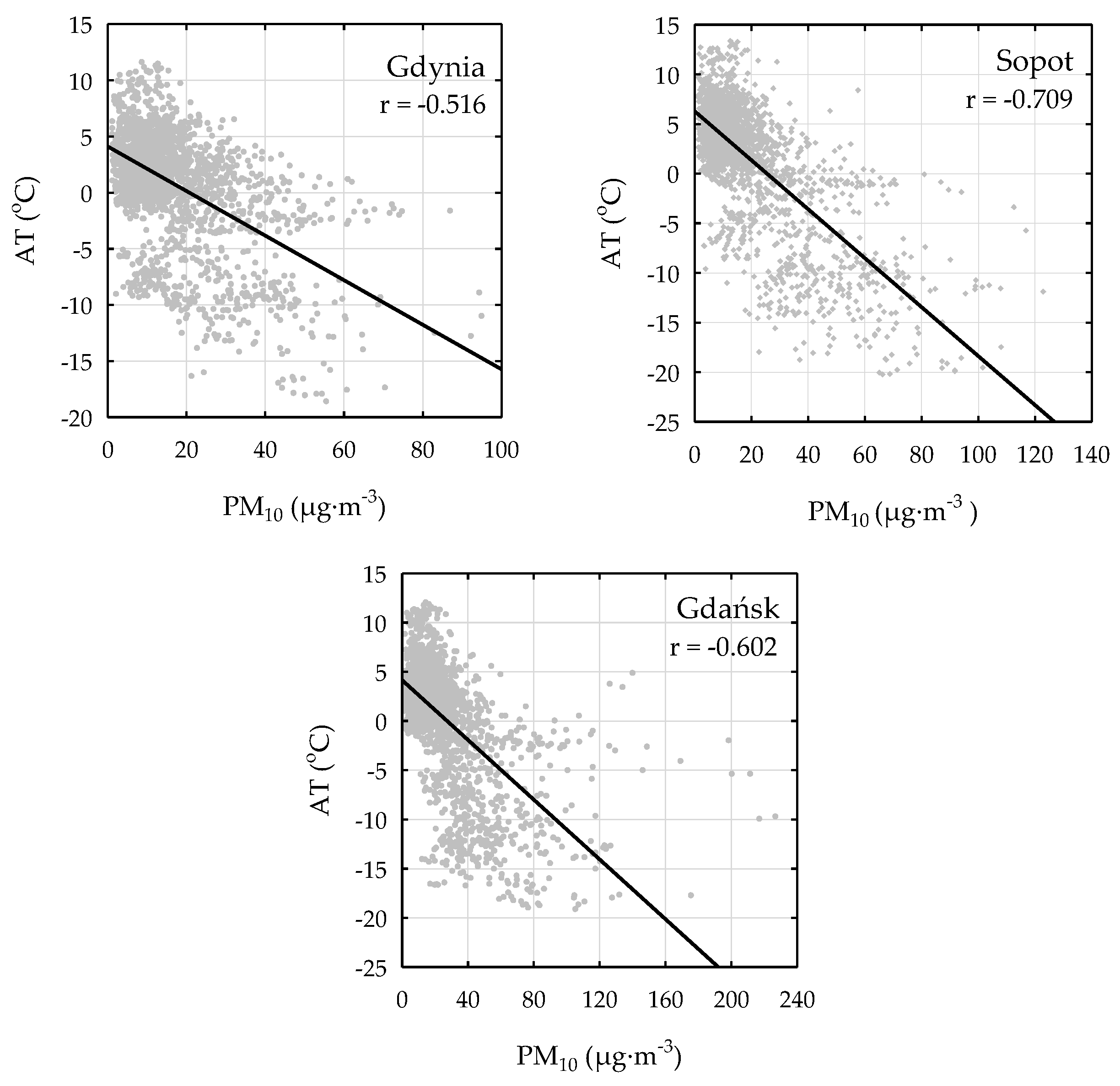
Even though the agglomeration of Tricity is one of the regions in Poland characterised by, on average, the lowest particulate matter pollution, almost every winter, the recorded concentrations exceed the EU 24 h limit value for PM10 [20,27,39,49]. High PM10 concentrations, as well as those exceeding the standards set by the EU limit value, are recorded predominantly during the heating seasons and mainly result from the emissions due to combustion for energy generation purposes [41], the intensity of which is determined by the course of the air temperature. This is illustrated in Figure 2 which shows the temporal variations of seasonal PM10 and the air temperature in particular winter seasons, at the same time, indicating the interdependence of the two values. In the analysed winter seasons, the highest negative correlation between the PM10 values and the air temperature was determined in the season of 2011/2012 (Gdynia r = −0.516; Sopot r = −0.709; Gdańsk r = −0.602), shown in Figure 3, followed by the winter season of 2005/2006 (Gdynia r = −400; Sopot r = −459; Gdańsk r = −0.482). The causal link between the air temperature and the PM10 concentrations is recognized and described in detail in the literature on the subject, and also for the conditions found in the Tricity Agglomeration [27,37,49]. Generally, the most unfavourable conditions of air quality occur in winter during anticyclonic weather in which very low temperatures (≤0 °C), weak winds or calms, clear sky conditions, and a stable equilibrium in the atmosphere leads to the formation of temperature inversions [49]. The role of inversion in shaping PM10 concentrations in the winter seasons (D, J, F) in the years of 2004/2005–2012/2013 in Tricity was presented by Czarnecka and Nidzgorska-Lencewicz [39]. The results obtained by the authors show that the unfavourable conditions for PM10 dispersion in the lower troposphere were mainly determined by the elevated inversion which occurred with comparable (almost 90%) frequency both during the day as well as night. However, a predominant role was played by the altitude of the base of the daytime elevated inversion.
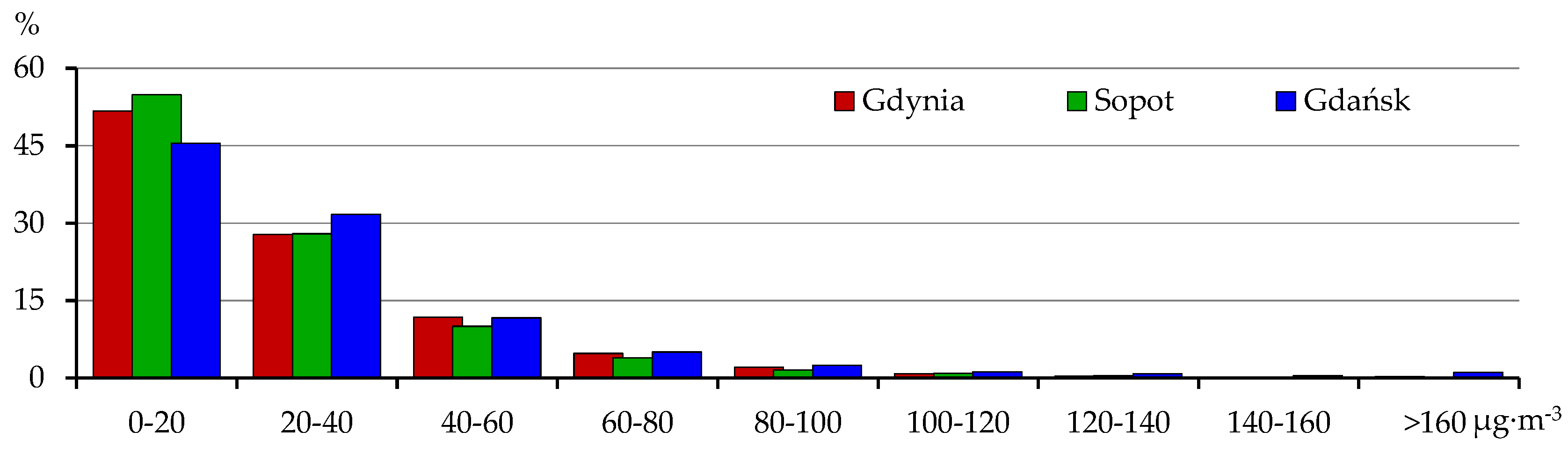
A histogram presenting the frequency of the adopted ranges of hourly concentrations recorded in the analysed winter seasons complements the characteristics of the PM values (Figure 4). Generally, the similarity of the distribution of the adopted ranges of concentrations is notable. Regardless of the particular station, the predominant concentrations are within the range of 0–20 μg·m−3, which, in Gdynia, Sopot, and Gdańsk, occur with a frequency of 55–45%. The cases of hourly concentrations over 100 μg·m−3 occurred in Sopot and Gdynia with a frequency of no more than 1.8% and, in Gdańsk, approximately twice more often. The distribution of the hourly PM10 concentration presented above is characteristic for the whole region of northern Poland, as was shown by Rawicki et al. [50].
3.2. Artificial Neural Networks
There are many types and variants of neural networks which differ in structure and way of operation, but the most common types of ANNs used in forecasting studies are multilayer perceptron neural networks (MLP-ANN) which are constructed with three layers: input, hidden, and output layers. Keeping in mind the results obtained by other authors [22,23,26,31,32,46] who, using MLP models, successfully predicted PM10 concentrations, in the current study, the ANN-MLP models have been applied in order to forecast hourly concentrations of particulate matter in three stations in Tricity. The input variable to the model consisted of hourly values of the PM10 concentrations, air temperature, relative humidity, atmospheric pressure, and wind speed. In the selection of input variables, the ANN-MLP models have been suggested by previous studies [20,27,31,37,38,40,45] and our understanding of atmospheric processes. However, data availability limitations needed to be taken into account. For the purpose of training the network, learning algorithms belonging to quasi-Newton methods were used, that is, the error back propagation algorithm and the Broyden–Fletcher–Goldfarb–Shanno (BFGS) algorithm. In terms of the analysed data, the optimum activation function (identity, logistic, tangent-hyperbolic, or exponential) was obtained using the Automated network search. This module is an extremely useful tool which facilitates the most tedious and time-consuming stage of establishing neural networks: the testing and selecting of different models. Each ANN was trained with 20 initialisations to ensure that they best fit the concentrations [51].
The analysis of ANNs undergoes three phases, the training, testing, and validation of the data, to which 70%, 15%, and 15% of the data was assigned randomly [26,45]. The training subset is used to estimate and learn the parameter’s patterns in the data point. Since ANNs are extremely versatile estimators of data which, following the appropriate number of iterations, can be allocated to almost every dataset, including insignificant noise (PM10 concentration time series data that are typically noisy and contain outliers) and experimental errors, the process of network learning was controlled by validating the subset which is used to evaluate the generalization ability of the supposedly trained network. In other words, the model is trained only to the point when the decrease in the prediction error for a given training set is accompanied by a decrease in the prediction error for the validating set. The test subset (not included in the training of the model) is responsible for performing the final check on the trained network.
Finally, models allowing for the prediction of PM10 concentration from 1 to 6 h in advance were created. The analysis was initiated by training the 20 models for each variant, out of which the Automated network search selected 5 models with the best fitting PM10 concentrations. In this way, a total of 90 models were selected (30 for each station) which were later assessed according to the adopted performance criteria. The quality of the obtained models was assessed by analysing the error rate expressed by the IA, FB, RMSE, and R2 values described in Section 2.3 and individually calculated for the training, validating, and testing set. The results of the particular models constituted the grounds for selecting one model for each time frame characterised by the best fitting parameters in terms of the test data. Accordingly, Table 2 presents the best structures for the hourly models and ANN topologies in the form of input-hidden-output neuron count. In this work, 3–11 neurons in the hidden layer have been tried. On the whole, almost 2/3 of the obtained models generated the best results with 9, 10, or 11 neurons in the hidden layer. The data presented in Table 2 show that the tangent-hyperbolic function was the most common activation function in the hidden layer and that the exponential function was the most common activation function for the output layer.
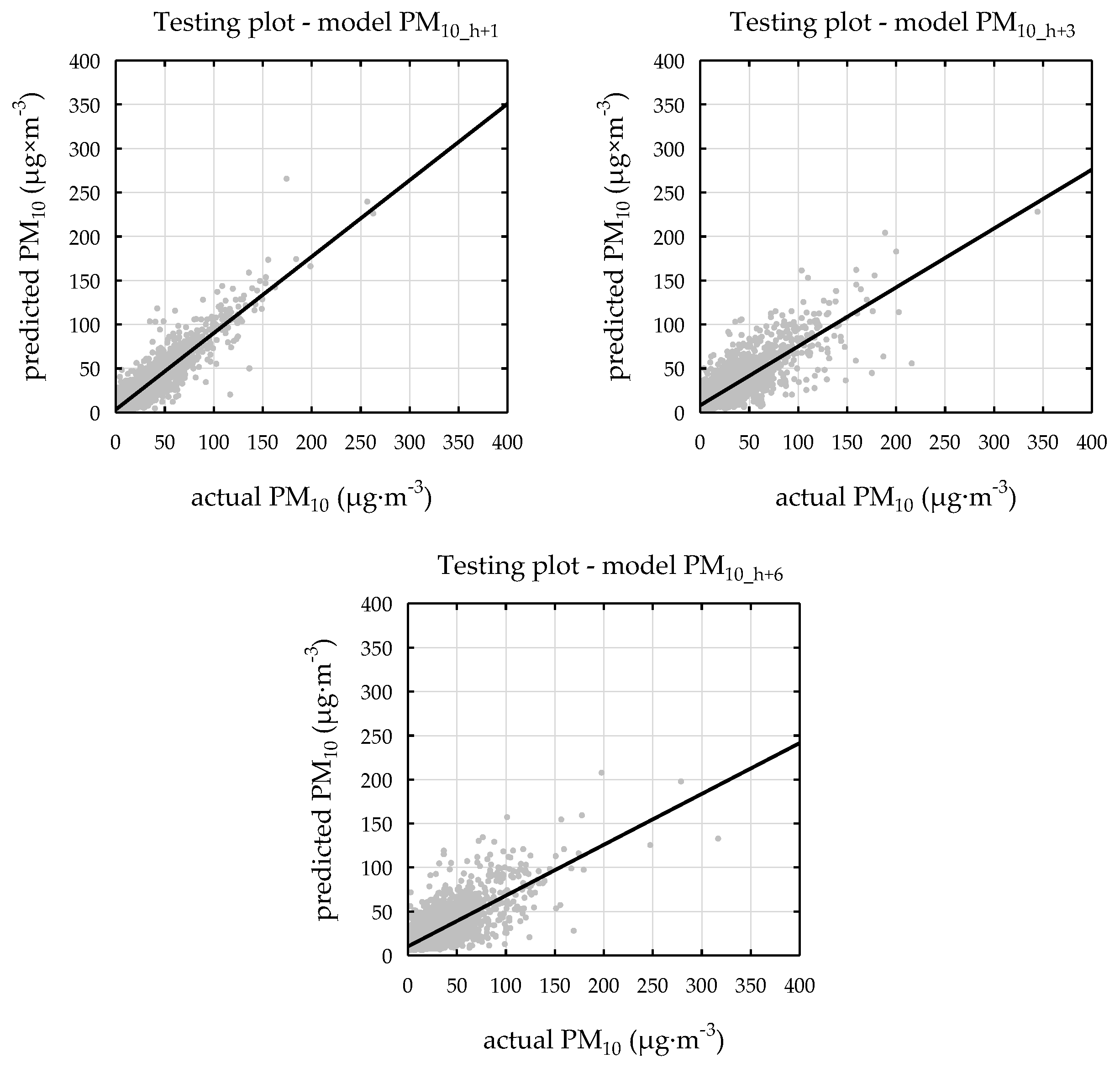
The obtained ANN models showed that the overall agreement in training denoted by IA between the modelled and observed values varied in the range of 0.802–0.956, the RMSE values ranged from 9.32 to 22.82, and the R2 values ranged from 0.487 to 0.844. In comparison to the training subset, the statistical parameters for the test and validation sets showed slightly lower values of IA (except for the PM10_h+1 and PM10_h+2 models for Gdańsk), whereas the RMSE, depending on the analysed variant and station, showed lower or higher values. In turn, as for R2, the values obtained in the test series were higher compared to the training series for Sopot and Gdańsk, as is presented in Table 2. In all three stations, the best agreement of IA was within the range of 0.944–0.956 with R2 in the range of 0.805–0.844, found for the PM10_h+1 model, that is, the shortest forecast of 1 h. The longer the time covered by the prognosis, the smaller the ability of the model to generate a forecast. This is illustrated by the scatter plots in Figure 5, showing the conformity of the models’ results in testing the subsets; the actual versus predicted values of the hourly PM10 levels in Sopot for the PM10_h+1 and PM10_h+6 models. Regardless of the analysed time variant and station, the FB values obtained from the estimate ANN models varied around 0. This means that the discussed models did not show a tendency to over-predict and under-predict the hourly PM10 concentrations. Additionally, this shows that no systematic errors are made even if random errors are present [51].
Out of the three analysed stations, by far the best results were obtained for Sopot. All the ANN models were characterised by superior results of the tests in the test subset, the IA, and the R2, respectively, in the ranges of 0.957–0.811 and 0.578–0.848 with the smallest RMSE error ranging from 8.80 to 14.96. The poorest test results were obtained for the models generated for the Gdańsk station, mainly due to the highest values of the RMSE. Undoubtedly, this is connected with not only the, on average, highest PM10 concentrations recorded in this station, but also with their very high variability. The SD values given in Table 1 show approximately 40% and 33% greater fluctuation rates in the hourly PM10 concentrations, as compared with Sopot and Gdynia, respectively. Such a high variability is also clearly illustrated in Figure 2, showing a generally greater range of outliers and extremes values, particularly in the seasons 2002/2003, 2005/2006, and 2009/2010. Even though ANNs are considered very good estimators and generally allow for more accurate predictions than traditional linear statistical approaches, as has already been discussed, it is worthwhile to keep in mind that the high variability in data may affect the obtained results. This was proven by Taşpınar [23] who, differentiating the data series into the winter and summer data subsets, obtained better test parameters for the ANN models.
Generally, keeping in mind the results of the tests, as well as the relatively low number of input variables, the obtained ANN models can be considered satisfactory. Using ANNs on the basis of 8 variables (7 meteorological elements and PM10 concentration) Grivas and Chaloulakou [45] developed models showing the predictive ability for 24-h-in-advance hourly PM10 concentrations at four sampling locations of different types in Athens (Greece). The authors concluded that the obtained results were rather satisfactory, with values of R2 for the independent test sets ranging between 0.50 and 0.67 for the four sites and values of the IA ranging between 0.80 and 0.89. Additionally, they stated that the performance of the examined neural network models was superior in comparison with the multiple linear regression models that were developed in parallel. Similarly, on the basis of different combinations of 5 variables (4 meteorological elements, and PM10 concentration), Taşpınar [23] obtained seasonal ANN models for the prediction of the daily average PM10 one day ahead in Düzce, Turkey. The agreement in this winter model in training between the modelled and observed values varied in the range of 0.78–0.83 and the R2 values ranged in the range of 0.693–0.722. Additionally, the high values of the index of the agreement between the measured and modelled daily averaged PM10 concentrations, between 0.80 and 0.85, for the forecasting of the daily averaged PM10 in Thessaloniki (Greece) and Helsinki (Finland) were presented by Voukantsis et al. [31]. However, it must be emphasized that the input data set to the ANN models comprised the concentrations of the other pollutants as well, apart from the meteorological elements. It is appropriate to list the results by Hooyberghs et al. [52] on forecasting the daily average PM10 concentrations in Belgium one day ahead with the use of ANN, where the authors used, in their first attempt (model), the boundary layer height and concentrations of the PM10 concentration, gradually increasing the accuracy of the forecast by taking into account the cloud cover, the day of the week, and the wind direction.
4. Conclusions
The main goal of this study was to predict PM10 levels 1 to 6 h ahead. It was shown that ANNs have been proven to be effective prediction techniques for modelling the hourly distribution of PM10 at the Agglomeration of Tricity (Poland) during the winter seasons. The input data in the form of basic meteorological elements and PM10 concentration with use of a multi-layer perceptron ANN (ANN-MLP) appeared to be promising in the testing subset for the three stations with R2 values in the range of 0.452–0.848, IA in the range of 0.693–0.957, and RMSE values in the range of 8.80–23.56. Moreover, the tested models did not show a tendency towards over-predicting or under-predicting the hourly PM10 level. The capability of these techniques to predict PM10 concentrations was certainly the highest for the time of 1 h in advance and the lengthening of the time of prognosis (to 6 h in advance) resulted in a decrease in the capability to generate the forecast. The highest agreement in the training, validating, and testing subset was found for models for Sopot—the station with the average lowest concentrations and variability of PM10 level in the winter season.
The ability to accurately model and predict the ambient concentration of PM10 is essential for effective air quality management and the development of policies relating to air quality. The obtained models can be used in the emergency population warning systems, indicating situations which could potentially cause direct threats to human health.
The ability to accurately model and predict the ambient concentration of PM10 is essential for effective air quality management and policies development.
For future work, I will also enhance the effectiveness of the ANNs by integrating the mechanism of hybrid approaches.
Acknowledgments
The author would like to thank ARMAAG for making the data accessible.
Conflicts of Interest
The authors declare no conflict of interest.
References
- Philip, S.; Martin, R.V.; van Donkelaar, A.; Lo, J.W.-H.; Wang, Y.; Chen, D.; Zhang, L.; Kasibhatla, P.S.; Wang, S.; Zhang, Q.; et al. Global chemical composition of ambient fine particulate matter for exposure assessment. Environ. Sci. Technol. 2014, 48, 13060–13068. [Google Scholar] [CrossRef] [PubMed]
- Taiwo, A.M.; Beddows, D.C.S.; Shi, Z.; Harrison, R.M. Mass and number size distributions of particulate matter components: Comparison of an industrial site and an urban background site. Sci. Total Environ. 2014, 475, 29–38. [Google Scholar] [CrossRef] [PubMed]
- Samek, L.; Stegowski, Z.; Furman, L. Preliminary PM2.5 and PM10 fractions source apportionment complemented by statistical accuracy determination. Nukleonika 2016, 61, 75–83. [Google Scholar] [CrossRef]
- Almeida, S.M.; Pio, C.A.; Freitas, M.C.; Reis, M.A.; Trancoso, M.A. Approaching PM2.5 and PM2.5–10 source apportionment by mass balance analysis, principal component analysis and particle size distribution. Sci. Total Environ. 2006, 368, 663–674. [Google Scholar] [CrossRef] [PubMed]
- Eleftheriadis, K.; Oschenkuhn, K.M.; Lymperopoulou, T.; Karanasiou, A.; Razos, P.; Ochsenkuhn-Petropoulou, M. Influence of local and regional sources on the observed spatial and temporal variability of size resolved atmospheric aerosol mass concentrations and water-soluble species in the Athens metropolitan area. Atmos. Environ. 2014, 97, 252–261. [Google Scholar] [CrossRef]
- Majewski, G.; Rogula-Kozłowska, W. The elemental composition and origin of fine ambient particles in the largest Polish conurbation: First results from the short-term winter campaign. Theor. Appl. Climatol. 2016, 125, 79–92. [Google Scholar] [CrossRef]
- Brunekreef, B.; Holgate, S.T. Air pollution and health. Lancet 2002, 360, 1233–1242. [Google Scholar] [CrossRef]
- Kappos, A.D.; Bruckmann, P.; Eikmann, T.; Englert, N.; Heinrich, U.; Hoppe, P.; Koch, E.; Krause, G.H.M.; Kreyling, W.G.; Rauchfuss, K.; et al. Health effects of particles in ambient air. Int. J. Hyg. Environ. Health 2004, 207, 399–407. [Google Scholar] [PubMed]
- Medina, S.; Plasencia, A.; Ballester, F.; Mucke, H.G.; Schwartz, J. Apheis: Public health impact of PM10 in 19 European cities. J. Epidemiol. Commun. Health 2004, 58, 831–836. [Google Scholar] [CrossRef] [PubMed]
- Wilson, J.G.; Kingham, S.; Pearce, J.; Sturman, A.P. A review of intraurban variation in particulate air pollution: Implications for epidemiological research. Atmos. Environ. 2005, 39, 6444–6462. [Google Scholar] [CrossRef]
- Dominici, F.; Peng, R.D.; Bell, M.L.; Pham, L.; McDermott, A.; Zeger, S.L.; Samet, J.M. Fine particulate air pollution and hospital admission for cardiovascular and respiratory diseases. JAMA 2006, 295, 1127–1134. [Google Scholar] [CrossRef] [PubMed]
- Freitas, M.C.; Pacheco, A.M.G.; Verburg, T.G.; Wolterbeek, H.T. Effect of particulate matter, atmospheric gases, temperature, and humidity on respiratory and circulatory diseases’ trends in Lisbon, Portugal. Environ. Monit. Assess. 2010, 162, 113–121. [Google Scholar] [CrossRef] [PubMed]
- Shi, L.; Zanobetti, A.; Kloog, I.; Coull, B.A.; Koutrakis, P.; Melly, S.J.; Schwartz, J.D. Low-concentration PM2.5 and mortality: Estimating acute and chronic effects in a population-based study. Environ. Health Perspect. 2015, 124, 46. [Google Scholar] [CrossRef] [PubMed]
- Widziewicz, K.; Rogula-Kozłowska, W.; Loska, K.; Kociszewska, K.; Majewski, G. Health Risk Impacts of Exposure to Airborne metals and Benzo(A)Pyrene during Episodes of High PM10 Concentrations in Poland. Biomed. Environ. Sci. 2018, 31, 323–332. [Google Scholar] [CrossRef]
- Zwozdziak, A.; Gini, M.I.; Samek, L.; Rogula-Kozlowska, W.; Sowka, I.; Eleftheriadis, K. Implications of the aerosol size distribution modal structure of trace and major elements on human exposure, inhaled dose and relevance to the PM2.5 and PM10 metrics in a European pollution hotspot urban area. J. Aerosol Sci. 2017, 103, 38–52. [Google Scholar] [CrossRef]
- Lim, S.S.; Vos, T.; Flaxman, A.D.; Danaei, G.; Shibuya, K.; Adair-Rohani, H.; AlMazroa, M.A.; Amann, M.; Anderson, H.R.; Andrews, K.G.; et al. A comparative risk assessment of burden of disease and injury attributable to 67 risk factors and risk factor clusters in 21 regions, 1990–2010: A systematic analysis for the Global Burden of Disease Study 2010. Lancet 2012, 380, 2224–2260. [Google Scholar] [CrossRef]
- European Environment Agency. Air Quality in Europe—2017 Report; European Environment Agency: Copenhagen, Denmark, 2017. [Google Scholar]
- Organization for Economic Cooperation and Development. Environmental Outlook to 2050, the Consequences of Inaction. In Organisation for Economic Co-Operation and Development Publishing; Organization for Economic Cooperation and Development: Paris, France, 2012. [Google Scholar]
- Kukkonen, J.; Pohjola, M.; Sokhi, R.S.; Luhana, L.; Kitwiroon, N.; Fragkou, L.; Rantamäki, M.; Berge, E.; Ødegaard, V.; Slørdal, L.H.; et al. Analysis and evaluation of selected local-scale PM10 air pollution episodes in four European cities: Helsinki, London, Milan and Oslo. Atmos. Environ. 2005, 39, 2759–2773. [Google Scholar] [CrossRef]
- Czarnecka, M.; Nidzgorska-Lencewicz, J. Impact of weather conditions on winter and summer air quality. Int. Agrophys. 2011, 25, 7–12. [Google Scholar]
- Shahraiyni, H.T.; Sodoudi, S. Statistical Modeling Approaches for PM10 Prediction in Urban Areas; A Review of 21st-Century Studies. Atmosphere 2016, 7, 15. [Google Scholar] [CrossRef]
- Whalley, J.; Zandi, S. Particulate matter sampling techniques and data modelling methods. In Air Quality-Measurement and Modeling; INTECH: Morn Hill, UK, 2016; pp. 29–54. [Google Scholar] [CrossRef]
- Taşpınar, F. Improving artificial neural network model predictions of daily average PM10 concentrations by applying principle component analysis and implementing seasonal models. J. Air Waste Manag. Assoc. 2015, 65, 800–809. [Google Scholar] [CrossRef] [PubMed]
- Ul-Saufie, A.Z.; Yahaya, A.S.; Ramli, N.A.; Rosaida, N.; Hamid, H.A. Future daily PM10 concentrations prediction by combining regression models and feedforward backpropagation models with principle component analysis (PCA). Atmos. Environ. 2013, 77, 621–630. [Google Scholar] [CrossRef]
- Sayegh, A.S.; Munir, S.; Habeebullah, T.M. Comparing the performance of statistical models for predicting PM10 concentrations. Aerosol Air Qual. Res. 2014, 14, 653–665. [Google Scholar] [CrossRef]
- Taşpınar, F.; Bozkurt, Z. Application of artificial neural networks and regression models in the prediction of daily maximum PM10 concentration in Düzce, Turkey. Fresenius Environ. Bull. 2014, 23, 2450–2459. [Google Scholar]
- Czarnecka, M.; Nidzgorska-Lencewicz, J. Application of cluster analysis in defining the meteorological conditions shaping the variability of PM10 concentration. Annu. Set Environ. Prot. 2015, 17, 40–61. [Google Scholar]
- Nazif, A.; Mohammed, N.I.; Malakahmad, A.; Abualqumboz, M.S. Application of step wise regression analysis in predicting future particulate matter concentration episode. Water Air Soil Pollut. 2016, 227, 117. [Google Scholar] [CrossRef]
- Qiao, J.; Cai, J.; Han, H.; Cai, J. Predicting PM2.5 concentrations at a regional background station using second order self-organizing fuzzy neural network. Atmosphere 2017, 8, 10–17. [Google Scholar] [CrossRef]
- Pires, J.; Martins, F.; Sousa, S.; Alvim-Ferraz, M.; Pereira, M. Prediction of the daily mean PM10 concentrations using linear models. Am. J. Environ. Sci. 2008, 4, 445–453. [Google Scholar] [CrossRef]
- Voukantsis, D.; Karatzas, K.; Kukkonen, J.; Räsänen, T.; Karppinen, A.; Kolehmainen, M. Intercomparison of air quality data using principal component analysis, and forecasting of PM10 and PM2.5 concentrations using artificial neural networks, in Thessaloniki and Helsinki. Sci. Total Environ. 2011, 409, 1266–1276. [Google Scholar] [CrossRef] [PubMed]
- Azid, A.; Juahir, H.; Toriman, M.E.; Kamarudin, M.K.A.; Saudi, A.S.M.; Hasnam, C.N.C.; Aziz, N.A.A.; Fazureen Azaman, F.; Latif, M.T.; Zainuddin, S.F.M.; et al. Prediction of the Level of Air Pollution Using Principal Component Analysis and Artificial Neural Network Techniques: A Case Study in Malaysia. Water Air Soil Pollut. 2014, 225, 2063. [Google Scholar] [CrossRef]
- Demuzere, M.; Trigo, R.M.; Vila-Guerau de Arellano, J.; van Lipzig, N.P.M. The impact of weather and atmospheric circulation on O3 and PM10 levels at a rural mid-latitude site. Atmos. Chem. Phys. 2009, 9, 2695–2714. [Google Scholar] [CrossRef]
- İçağa, Y.; Sabah, E. Statistical analysis of air pollutants and meteorological parameters in Afyon, Turkey. Environ. Model. Assess. 2009, 14, 259–266. [Google Scholar] [CrossRef]
- Leśniok, M.; Caputa, Z. The role of atmospheric circulation in air pollution distribution in Katowice Region (Southern Poland). Int. J. Environ. Waste Manag. 2009, 4, 62–74. [Google Scholar] [CrossRef]
- Unal, Y.S.; Toros, H.; Deniz, A.; Incecik, S. Influence of meteorological factors and emission sources on spatial and temporal variations of PM10 concentrations in Istanbul metropolitan area. Atmos. Environ. 2011, 45, 5504–5513. [Google Scholar] [CrossRef]
- Nidzgorska-Lencewicz, J.; Czarnecka, M. Winter weather conditions vs. air quality in Tricity, Poland. Theor. Appl. Climatol. 2015, 119, 611–627. [Google Scholar] [CrossRef]
- Li, Y.; Chen, Q.; Zhao, H.; Wang, L.; Tao, R. Variations in PM10, PM2.5 and PM1.0 in an urban area of the Sichuan Basin and their relation to meteorological factors. Atmosphere 2015, 6, 150–163. [Google Scholar] [CrossRef]
- Czarnecka, M.; Nidzgorska-Lencewicz, J. The impact of thermal inversion on the variability of PM10 concentration in winter seasons in Tricity. Environ. Prot. Eng. 2017, 43, 157–172. [Google Scholar]
- Czernecki, B.; Półrolniczak, M.; Leszek Kolendowicz, L.; Marosz, M.; Kendzierski, S.; Pilguj, N. Influence of the atmospheric conditions on PM10 concentrations in Poznań, Poland. J. Atmos. Chem. 2017, 74, 115–139. [Google Scholar] [CrossRef]
- Reizer, M.; Juda-Rezler, K. Explaining the high PM10 concentrations observed in Polish urban areas. Air Qual. Atmos. Health 2016, 9, 517–531. [Google Scholar] [CrossRef] [PubMed]
- Central Statistical Office. Available online: http://stat.gov.pl (accessed on 20 February 2018).
- Państwowy Monitoring Środowiska, Inspekcja Ochrony Środowiska. The Air Quality Assesment in Zones in Poland for 2016, Warsaw 2017 (in Polish). Available online: https://powietrze.gios.gov.pl/pjp/documents/download/102460 (accessed on 20 March 2018).
- Directive CAFÉ. Available online: https://eur-lex.europa.eu/legal-content/PL/TXT/?uri=CELEX%3A32008L0050 (accessed on 20 February 2018).
- Grivas, G.; Chaloulakou, A. Artificial neural network models for prediction of PM10 hourly concentrations, in the Greater Area of Athens, Greece. Atmos. Environ. 2006, 40, 1216–1229. [Google Scholar] [CrossRef]
- Yan Chan, K.; Jian, L. Identification of significant factors for air pollution levels using a neural network based knowledge discovery system. Neurocomputing 2013, 99, 564–569. [Google Scholar] [CrossRef]
- Hanna, S.; Chang, J. Acceptance criteria for urban dispersion model evaluation. Meteorol. Atmos. Phys. 2012, 116, 133–146. [Google Scholar] [CrossRef]
- Juda-Rezler, K.; Reizer, M.; Oudinet, J.P. Determination and analysis of PM10 source apportionment during episodes of air pollution in Central Eastern European urban areas: The case of wintertime 2006. Atmos. Environ. 2011, 45, 6557–6566. [Google Scholar] [CrossRef]
- Jędruszkiewicz, J.; Czernecki, B.; Marosz, M. The variability of PM10 and PM2.5 concentrations in selected Polish agglomerations: The role of meteorological conditions, 2006–2016. Int. J. Environ. Health Res. 2017, 27, 441–462. [Google Scholar] [CrossRef] [PubMed]
- Rawicki, K.; Czarnecka, M.; Nidzgorska-Lencewicz, J. Regions of pollution with particulate matter in Poland. E3S Web Conf. 2018, 28, 01025. [Google Scholar] [CrossRef]
- Lauret, P.; Heymes, F.; Forestierb, S.; Laurent Aprina, L.; Peyb, A.; Perrin, M. Forecasting powder dispersion in a complex environment using Artificial Neural Networks. Process Saf. Environ. Prot. 2017, 110, 71–76. [Google Scholar] [CrossRef]
- Hooyberghs, J.; Mensink, C.; Dumont, G.; Fierens, F.; Brasseur, O. A neural network forecast for daily average PM10 concentrations in Belgium. Atmos. Environ. 2005, 39, 3279–3289. [Google Scholar] [CrossRef]
Figure 1.
The location of the measuring stations in Agglomeration of Tricity (Poland).
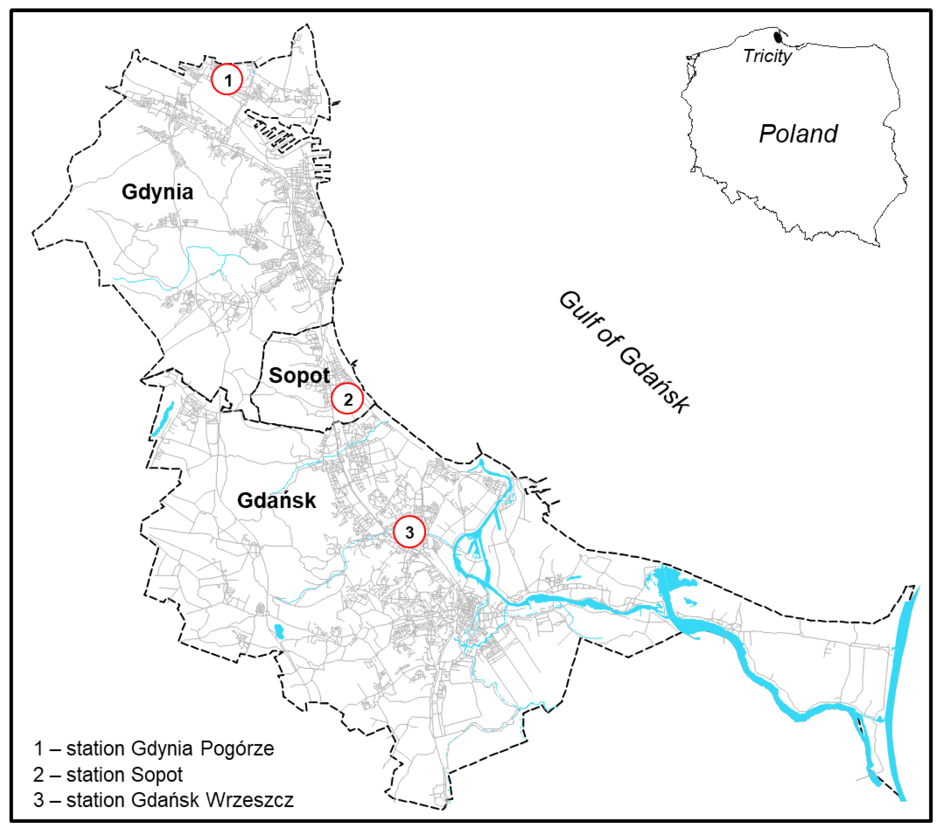
Figure 2.
The distribution of the hourly air temperature (a) and PM10 concentrations (b) in the Agglomeration of Tricity during the winter seasons (D, J, F) from 2002/2003 to 2016/2017. Notes: the boxes show the 25th, 50th, and 75th percentiles; the whiskers show the non-outlier range.
Figure 2.
The distribution of the hourly air temperature (a) and PM10 concentrations (b) in the Agglomeration of Tricity during the winter seasons (D, J, F) from 2002/2003 to 2016/2017. Notes: the boxes show the 25th, 50th, and 75th percentiles; the whiskers show the non-outlier range.

Figure 3.
The correlation between the air temperature and PM10 concentration in the Agglomeration of Tricity during the winter seasons of 2011/2012.
Figure 3.
The correlation between the air temperature and PM10 concentration in the Agglomeration of Tricity during the winter seasons of 2011/2012.

Figure 4.
The frequency distribution of hourly concentrations of PM10 in the Agglomeration of Tricity during the winter seasons (D, J, F) in 2002/2003–2016/2017.
Figure 4.
The frequency distribution of hourly concentrations of PM10 in the Agglomeration of Tricity during the winter seasons (D, J, F) in 2002/2003–2016/2017.

Figure 5.
The testing performance plots of artificial neural networks (ANN) models (PM10_h+1; PM10_h+3; PM10_h+6) in Sopot.
Figure 5.
The testing performance plots of artificial neural networks (ANN) models (PM10_h+1; PM10_h+3; PM10_h+6) in Sopot.


Table 1.
The basic statistics for PM10 and the meteorological elements for each station in the Agglomeration of Tricity during the winter seasons of 2002/2003–2016/2017.
Table 1.
The basic statistics for PM10 and the meteorological elements for each station in the Agglomeration of Tricity during the winter seasons of 2002/2003–2016/2017.
| Variable | Mean | Min | Max | SD |
|---|---|---|---|---|
| Gdynia Pogórze | ||||
| PM10 (μg·m−3) | 26.81 | 1.00 | 324.35 | 24.59 |
| AT (°C) | 1.04 | −18.55 | 14.00 | 4.46 |
| RH (%) | 80.86 | 30.20 | 100.00 | 11.29 |
| PRES (hPa) | 1006.67 | 960.10 | 1047.95 | 13.68 |
| WS (m·s−1) | 1.92 | 0.02 | 8.55 | 1.25 |
| Sopot | ||||
| PM10 (μg·m−3) | 25.13 | 1.00 | 375.7 | 23.39 |
| AT (°C) | 1.26 | −21.40 | 14.45 | 5.00 |
| RH (%) | 82.27 | 30.37 | 100.00 | 10.09 |
| PRES (hPa) | 1008.77 | 964.10 | 1045.60 | 12.30 |
| WS (m·s−1) | 1.92 | 0.03 | 8.00 | 1.14 |
| Gdańsk Wrzeszcz | ||||
| PM10 (μg·m−3) | 31.10 | 1.00 | 599.75 | 32.85 |
| AT (°C) | 0.48 | −19.95 | 13.85 | 5.03 |
| RH (%) | 82.38 | 31.90 | 100.00 | 9.66 |
| PRES (hPa) | 1011.40 | 962.80 | 1043.25 | 12.32 |
| WS (m·s−1) | 2.16 | 0.03 | 8.95 | 1.24 |
AT—air temperature; RH—relative humidity; PRES—atmospheric pressure; WS—wind speed; SD—standard deviation.
Table 2.
The statistics for the best performing ANN models for the forecasting of hourly concentrations of PM10.
Table 2.
The statistics for the best performing ANN models for the forecasting of hourly concentrations of PM10.
| ANN Models | Topology | Activation Function for Hidden Layer | Activation Function for Output Layer | IA | FB | RMSE | R2 | IA | FB | RMSE | R2 | IA | FB | RMSE | R2 |
|---|---|---|---|---|---|---|---|---|---|---|---|---|---|---|---|
| Train | Validation | Test | |||||||||||||
| Gdynia Pogórze | |||||||||||||||
| PM10_h+1 | 5-8-1 | Logistic | Exponential | 0.944 | 0.00 | 10.91 | 0.805 | 0.939 | 0.00 | 11.09 | 0.803 | 0.934 | −0.02 | 10.80 | 0.783 |
| PM10_h+2 | 5-7-1 | Logistic | Identity | 0.901 | 0.00 | 13.81 | 0.686 | 0.889 | 0.01 | 13.72 | 0.706 | 0.888 | 0.00 | 12.91 | 0.673 |
| PM10_h+3 | 5-11-1 | Logistic | Exponential | 0.866 | 0.00 | 15.31 | 0.611 | 0.848 | 0.00 | 15.09 | 0.634 | 0.824 | 0.00 | 15.16 | 0.574 |
| PM10_h+4 | 5-9-1 | Logistic | Tanh | 0.837 | 0.00 | 16.52 | 0.552 | 0.786 | 0.00 | 15.94 | 0.553 | 0.806 | 0.00 | 16.33 | 0.540 |
| PM10_h+5 | 5-10-1 | Exponential | Tanh | 0.811 | 0.00 | 17.39 | 0.504 | 0.751 | 0.00 | 16.65 | 0.510 | 0.757 | 0.00 | 17.50 | 0.482 |
| PM10_h+6 | 5-10-1 | Tanh | Exponential | 0.802 | 0.00 | 17.45 | 0.487 | 0.724 | 0.00 | 17.76 | 0.499 | 0.693 | 0.02 | 18.15 | 0.452 |
| Sopot | |||||||||||||||
| PM10_h+1 | 5-10-1 | Tanh | Identity | 0.956 | 0.00 | 9.32 | 0.844 | 0.951 | 0.00 | 9.42 | 0.832 | 0.957 | 0.00 | 8.80 | 0.848 |
| PM10_h+2 | 5-8-1 | Tanh | Tanh | 0.924 | 0.00 | 11.78 | 0.749 | 0.909 | 0.00 | 11.94 | 0.721 | 0.921 | 0.00 | 11.26 | 0.758 |
| PM10_h+3 | 5-10-1 | Tanh | Exponential | 0.899 | 0.00 | 13.14 | 0.685 | 0.876 | −0.01 | 12.98 | 0.655 | 0.881 | 0.02 | 13.12 | 0.690 |
| PM10_h+4 | 5-7-1 | Logistic | Tanh | 0.876 | 0.00 | 14.19 | 0.632 | 0.847 | 0.00 | 14.02 | 0.600 | 0.855 | 0.01 | 13.97 | 0.643 |
| PM10_h+5 | 5-11-1 | Logistic | Exponential | 0.860 | 0.00 | 14.75 | 0.597 | 0.811 | +0.02 | 15.02 | 0.550 | 0.816 | 0.02 | 15.00 | 0.595 |
| PM10_h+6 | 5-11-1 | Tanh | Exponential | 0.846 | 0.00 | 14.97 | 0.565 | 0.816 | 0.04 | 15.36 | 0.532 | 0.811 | 0.02 | 14.90 | 0.578 |
| Gdańsk Wrzeszcz | |||||||||||||||
| PM10_h+1 | 5-6-1 | Tanh | Exponential | 0.950 | 0.00 | 13.41 | 0.825 | 0.953 | 0.00 | 13.90 | 0.842 | 0.954 | 0.00 | 13.37 | 0.846 |
| PM10_h+2 | 5-6-1 | Exponential | Identity | 0.902 | 0.00 | 17.85 | 0.694 | 0.906 | 0.00 | 17.97 | 0.732 | 0.906 | 0.00 | 17.33 | 0.730 |
| PM10_h+3 | 5-6-1 | Exponential | Logistic | 0.866 | 0.00 | 20.18 | 0.616 | 0.850 | 0.00 | 21.12 | 0.632 | 0.858 | 0.00 | 20.02 | 0.639 |
| PM10_h+4 | 5-9-1 | Exponential | Logistic | 0.833 | 0.00 | 22.02 | 0.551 | 0.820 | 0.00 | 21.93 | 0.562 | 0.828 | 0.00 | 21.04 | 0.572 |
| PM10_h+5 | 5-10-1 | Tanh | Tanh | 0.829 | 0.00 | 22.20 | 0.540 | 0.796 | 0.01 | 23.62 | 0.499 | 0.805 | 0.00 | 22.19 | 0.538 |
| PM10_h+6 | 5-9-1 | Tanh | Exponential | 0.812 | 0.00 | 22.82 | 0.507 | 0.761 | 0.02 | 23.93 | 0.483 | 0.765 | 0.01 | 23.56 | 0.504 |
ANN—artificial neural networks; IA—index of agreement; FB—fractional mean bias; RMSE—root mean square error; R2—coefficient of determination.
© 2018 by the author. Licensee MDPI, Basel, Switzerland. This article is an open access article distributed under the terms and conditions of the Creative Commons Attribution (CC BY) license (http://creativecommons.org/licenses/by/4.0/).
Share and Cite
MDPI and ACS Style
Nidzgorska-Lencewicz, J. Application of Artificial Neural Networks in the Prediction of PM10 Levels in the Winter Months: A Case Study in the Tricity Agglomeration, Poland. Atmosphere 2018, 9, 203. https://doi.org/10.3390/atmos9060203
AMA Style
Nidzgorska-Lencewicz J. Application of Artificial Neural Networks in the Prediction of PM10 Levels in the Winter Months: A Case Study in the Tricity Agglomeration, Poland. Atmosphere. 2018; 9(6):203. https://doi.org/10.3390/atmos9060203
Chicago/Turabian StyleNidzgorska-Lencewicz, Jadwiga. 2018. "Application of Artificial Neural Networks in the Prediction of PM10 Levels in the Winter Months: A Case Study in the Tricity Agglomeration, Poland" Atmosphere 9, no. 6: 203. https://doi.org/10.3390/atmos9060203
Note that from the first issue of 2016, this journal uses article numbers instead of page numbers. See further details here.