1. Introduction
The global natural aerosol system is dominated on an areal basis by remote oceanic processes driven by phytoplankton that lead to the formation of an array of chemical cloud condensation nucleus types [
1,
2,
3,
4,
5,
6]. Reduced compounds of biological origin also help set the bioavailability of certain nutrient elements transported from atmosphere to ocean [
7,
8]. However, marine biogenic emissions are highly heterogeneous in their ecological geography, and the substances themselves are formed by (and participate in) highly nonlinear chemical processing both below and above the sea surface. The materials serve as cloud condensation nuclei (CCN), which contribute to radiative forcing and limit our ability to predict climate sensitivity. The attendant influence on climate has traditionally been very difficult to quantity. Uncertainties abound, and they can be reduced only through validation based on comparisons of model output with a multitude of independent measurements. The cloud seeding activity of dimethylsulfide (DMS) that was hypothesized decades ago is one of the mechanisms with significant uncertainty in sea–air coupling. In the present work, we will use the well-known CLAW hypothesis (originally proposed by Robert Jay Charlson, James Lovelock, Meinrat Andreae and Stephen G. Warren, and the acronym comes from the first letter of their surnames) [
9] exhibited with DMS as a primary example of how benchmarking can be accomplished. We will show that the methodology developed for the International Land Model Benchmarking (ILAMB) project [
10], some of which are currently incorporated into the International Ocean Model Benchmarking (IOMB) package, can be adapted to validate not only traditional carbon cycling from the surface ocean to deep sea, but also aerosol precursor generation, along with their distributions and effects.
DMS is the focus of our discussion, but we also comment on the potential and requirements for extension to a variety of other organic compounds [
2,
11]. Reduced carbon enters the marine boundary layer in a variety of volatile and primary forms, and we briefly discuss the validation of models that will be inclusive of all natural organics, even though measurements tend to be scarce relative to those of the often-studied sulfide [
12,
13,
14]. It will also be sensible to post-validate the oceanic production processes against ship and aircraft-based datasets, which reflect the resulting chemical complexity [
15].
Our text is structured as follows. The background section overviews and motivates the general challenges associated with marine aerosol. We then briefly describe a geophysical context for the study of ocean-derived aerosol, which is the chemical environment of the surface sea plus boundary layer. This section is followed by a description of the open source automated software system that is now under development for the benchmarking of marine biogeochemical processes and feedbacks. A section on methods demonstrates the application of our new IOMB-derived suite to validate outputs from contemporary Earth System Models (ESMs), given the available observational datasets. In our results section, detailed analyses are performed as proof of principle, and we end with some discussion of ways to further advance the current autonomous system. We also outline some of the research areas that we have been able to identify, within which uncertainties might be reduced through the evaluation of marine and general natural aerosols.
1.1. Background
Even as several of the most crucial global biogeochemical cycles are being implemented in ESMs [
16,
17], remote aerosol remains a continuing challenge to the community. Uncertainty in the aerosol forcing and feedbacks associated with ocean biota have long been suspected contributors in the era of global change, due to their effects on particle chemistry and cloud albedo [
4,
9]. However, their complex ecological geography means they are extremely difficult to quantify. A related issue is the isolation of anthropogenic effects relative to any natural counterparts. Uncertainty in these areas undermines the continuing international effort to appropriately simulate the aerosol mitigation of the global greenhouse effect—or amplification, as the case may be [
4,
9]. Both primary and secondary atmospheric particulates influence cloud microphysical properties and ultimately impact incoming solar radiation and Earth’s albedo. Although anthropogenic emissions tend to dominate the net contributions of atmospheric particles to radiative forcing, about 90% by mass of the total global aerosol is of natural origin. Volcanoes, plant emissions, and marine sea–air fluxes all play a role. Uncertainty derived from these natural sources is responsible for roughly half the variance exhibited by aerosol forcing since the onset of the industrial era [
18].
On a net basis, the atmospheric aerosol leads to reflection of incoming shortwave radiation [
19,
20,
21]. Although much has been learned since this effect was originally recognized [
22], many questions are yet to be answered or even addressed. The most pressing regard the biology of cloud albedo, because it exerts strong leverage on the global radiation balance [
9,
18,
20]. Such issues limit our ability to predict climate sensitivity, for example due to the better-known and ever increasing atmospheric concentrations of greenhouse gases (GHGs). For decades now, there has been a singular focus on anthropogenic aerosol as a major uncertainty driver [
21,
23]. However, progress in quantifying climate sensitivity has been irregular, and attention gradually shifted toward the evaluation of natural emissions (volcanic aerosols, natural sulfate, sea salt, and others). There is a strong need to determine the baseline of pre-industrial emissions, as well as the uncertainties introduced by shifts in global biota over the past century [
18].
The marine environment is biologically active and a major player in the cycling of natural atmospheric aerosols due to its vast extent [
1]. The vertical transport of trace gases and particles from the global ocean surface into the lower atmosphere constitutes a constant dynamic maintaining and controlling aerosol loading in the marine boundary layer (MBL). The composition and strength of oceanic emissions control the formation of both primary and secondary aerosols in the MBL, ultimately dictating the magnitude of planetary scale cloud albedo [
9,
24]. There continue to be open questions concerning the atmospheric inventory of natural aerosols worldwide, such that marine precursor-to-cloud relationships are even less well constrained than the major greenhouse gas relationships. This leads to significant uncertainty in aerosol–cloud interactions and creates challenges for the representation of natural aerosol distributions and general oceanic climate in Earth System Models [
11,
25].
The biogenic volatile organic compounds (BVOCs) represent a crucial subset of the overall marine aerosol challenge. Vertical flux-transport of trace gases such as DMS, isoprene, and the monoterpenes influences the formation of secondary organic aerosols (SOA), which modify cloud microphysics [
9,
26]. Other modes of uncertainty regard the organic chemistry of less volatile constituents among the dissolved organics [
12]. Primary organic aerosols (POA) introduced along with sea spray are really marine macromolecules that are derived from the degradation of phytoplanktonic cells; otherwise, they are downstream oxidation products that are also high in molecular weight [
5,
6]. The collective marine organics SOA and POA are additionally important in influencing particle composition, hygroscopicity, and size distribution, and with them come the usual microphysical implications [
2,
11]. Over roughly the last decade, there have been major advances in the quantification of marine aerosol sources, and this has been in part because logistical barriers are being overcome [
15]. As aerosol uncertainties are steadily reduced in coming years, there will be parallel needs for both increased long-term field measurements and the assessment of simulations attempting to reproduce them.
The natural marine aerosol dominated by chloride and sulfate has noticeable direct and indirect effects on the climate. Aerosol components such as sea salt, soil dust, organic macromolecules, and natural sulfate are often hygroscopic and act as cloud condensation nuclei, thus modulating cloud reflectivity [
27,
28,
29]. However, emissions of dimethylsulfide and volcanic sulfate lead to the greatest impact on global radiative forcing, both as a consequence of albedo effects [
30]. The global cloud albedo effect that is attributable to sea salt is reported to be about −0.04 Wm
−2, while DMS-derived sulfate and volcanic sulfate contribute −0.76 Wm
−2and −0.61 Wm
−2, respectively [
30]. Despite this potential for net cooling, the situation is confounded by numerous nonlinearities. Cloud albedo does not respond in a simple manner to the source strength of natural precursors [
31], and this is partly because of the superposition of anthropogenic emissions. There has been general difficulty representing baseline emissions in the absence of industrial fingerprints [
18,
20].
To reduce uncertainties implied by the inclusion of natural particles in climate models, we need to access and exploit a variety of the available observational datasets. These will include surface ocean concentration measurements [
13,
14], the direct quantification of fluxes [
3,
32], the analysis of detailed organic chemistry [
2,
5,
6], and studies conducted from the atmosphere and space [
33,
34]. The community must determine the level of realism that can be attached to the current suite of climate models. It must eventually be possible to faithfully simulate not only the recent past, but also to extend into the future in the predictive sense. The aerosol knowledge base must improve in order to constrain the next generation of model development. There is currently a strong interest in the design and implementation of new metrics to evaluate and quantify biogeochemical uncertainties, and aerosol cycles are foremost among them.
As a general rule, the specific biological processes underlying biogeochemical transfer to and from the global ocean are insufficiently represented in most Earth System Models (ESMs) [
6,
35,
36]. The best known examples involve the trace greenhouse gas carbon dioxide, which currently demands almost an entire generation of validation effort, which has led to the community beginning to display confidence in its computed and globally distributed fluxes [
17]. Similarly however, surface ocean fluxes of marine aerosol precursors such as DMS are crucial to the planetary climate state. Uncertainty with regard to the effects of aerosol chemical composition on cloud albedo is also applicable to the SOA and POA, through their influence on sea spray and hygroscopicity [
2,
29]. Moreover, the organic chemistry also affects nutrient cycling [
8]. In the present work, we adopt DMS as the springboard to demonstrate means of automating the global aerosol validation effort, with discussions of the other issues included as well.
1.2. The Marine Atmospheric and Aerosol Environment
The marine boundary layer (MBL) is that part of the atmosphere closest to the ocean, extending from the ocean surface up to 100–1000 m above sea level. Within this subset of the planetary surface layer, ocean and atmosphere exchange heat and matter through turbulent fluid mechanical transport [
37]. Air–sea interactions are dynamically driven, as in the case of wind shear at the ocean surface, or thermodynamically driven, with respect to buoyancy. These interactions initiate the formation of primary sea salt and secondary non-sea-salt aerosols that could serve as nucleating agents. Cloud supersaturations in the order of 0.2% to 0.3% or even less are capable of activating aerosol in the accumulation mode (0.1–1.0 µm), forming the cloud droplets at the global scale and imparting their strong effects on reflectivity [
27]. An absence of anthropogenic and terrestrial aerosols over the far reaches of the open ocean leaves a clean marine environment, in which natural precursors serve as cloud condensation nuclei (CCN). Ultimately, they control the formation of low-level stratus and stratocumulus clouds [
38]. Albedo modification is thus partly driven by natural processes.
The study of biogeochemical cycling in the boundary layer regime has advanced steadily across the regional and global environment over the past few decades, bringing with it an enhanced appreciation for the complexity of marine climate feedbacks. Novel techniques for gathering field datasets come online continually [
15,
34], reinforcing ever-improving model structures in a positive cycle [
5,
6]. Innovative upper ocean biogeochemical mechanism designs have been particularly effective contributors. Simulations now extend from the original, simple foodweb concept to intricate processing that may require hundreds of state variables and multiple trace elemental cycles [
39,
40,
41,
42,
43,
44]. In some cases, detailed trace gas and aerosol precursor modules are now included [
4,
5,
45]. Increases in model complexity come with a downside, however: multiple layers of uncertainty are introduced into the analysis, and there are still more questions to be answered in terms of parameterizing marine aerosols in ESMs.
As the frontiers of computation meet up with modern analytical techniques (largely chemical and biological), there will be the need to apply continually updated constraints that are relative to observations at all scales. Disparities between model results and field data often raise the most critical questions, regarding for example the level of objective validation that has been attained, or the very reliability of current ESM structures [
11,
46]. To reduce uncertainties and improve model development, it is critical to validate and skill-test the surface ocean biogeochemistry that is now being rapidly incorporated into contemporary ESMs. We must continually reinvent our understanding of their fundamental capabilities [
47].
1.3. Automated Validation: Ocean Biogeochemical Regime
We have recently developed a set of ESM analysis methods and metrics specific to the marine biogeochemistry realm, as part of the ongoing International Ocean Model Benchmarking (IOMB) effort. This is with the intent to meet intensifying validation needs for biogeochemical modelers and measurement scientists within the ocean community. The tool is derived from the International Land Model Benchmarking (ILAMB), which is a closely related model validation project that is focused on terrestrial ecosystem dynamics [
10]. Our fundamental strategy is to automate the confrontation of ocean physics, biology, and chemistry simulations with a wealth of observational datasets. We refer to the full variety of analyses, from shipboard studies to remote sensing measurements. The IOMB package is already capable of assessing global light-driven nutrient uptake by phytoplankton (photosynthesis as represented by primary production). Furthermore, it has been extensively tested relative to global carbon budgets. Here, we explore the methods in a general manner, with extension to aerosol cycling.
We incorporate long-standing and newer observational datasets to evaluate simulation performance and guide future model development. The hope is to assist the international community in reducing marine biogeochemical uncertainty, and discovering the crucial links to indirect radiation effects [
2,
18,
21]. There is currently a handful of custom packages used by different modeling communities to benchmark model results, but IOMB presents the first objectively open access platform to the ocean community with complete freedom to benchmark any model with a chosen observational dataset. The emphasis here is placed upon tests for volatile sulfur as a subset of BVOCs, which still tend to be rare in ESM output. Strategies are discussed for enhancing sparse aerosol and precursor data sets through ecogeographic comparisons, and for making them more convenient to use and more readily available.
To date, only a handful of research groups have explored the concept of developing reasonable metrics to objectively validate ESM skill sets [
48,
49,
50,
51,
52]. There is still a need to sensitize the biogeochemistry and natural aerosol communities to the timeliness and importance of benchmarking, and thus constraining model outputs. Uncertainties must be reduced in support of future model development efforts; this is the major channel through which improvements can be achieved. A recent review showed that more than 60% of the marine biogeochemistry literature provides only a visual comparison between model results and field data. The result is especially striking when viewed in the following light: a mere 10% accepted the challenge of validating with effective statistical methods [
51]. Quantitative techniques are thus essential and timely at this point in the history of climate systems simulation. The statement remains true even if the strategies are taxing to implement; multiple spatial and temporal scales must be considered when comparing model output with the available field data or remotely-sensed distributions. Detailed benchmarks for the aerosol precursors and their marine sources are now required, and should be adapted systematically to constrain modeling activities.
2. Methods
Sea-air ventilation and the vertical transfer of trace greenhouse gases or marine aerosol precursors are closely associated with the dynamics of marine food webs, along with shifts in regional ecosystems [
4,
53,
54,
55,
56]. Thus, any shift in nutrient availability within the euphotic layer—coupled to changes in ambient conditions that could influence biomass production in a less direct manner—can affect gas or aerosol loadings in the lower troposphere. The core of our effort is thus focused necessarily upon the uppermost, sunlit layers of the ocean. However, remineralization injects inorganics into the water column at depth, and the associated recycling patterns reflect central ocean distributions, so that the sectional analysis approaches cannot be ignored.
Our International Ocean Model Benchmarking (IOMB) package constitutes open source software built on the Python programming language, and it is both currently and continually under development to benchmark the most relevant marine biogeochemical variables and processes. Our strategy is to aid in investigating the numerous, complex ocean biogeochemical feedbacks of the Earth system residing within the international suite of climate models. In some cases, we anticipate that large sections of important biogeochemical interactions will be entirely missing from computational representations. This is the essence of structural uncertainty, and it is part of our responsibility to identify such omissions. The goal is most easily accomplished by cross-comparing biogeochemical capabilities among modeling groups, and this will be a key component of the project.
The essential goal of our effort is to constrain future model developments by bringing available observational datasets to bear. Detailed documentation and a tutorial regarding the most recently released version 2.2 of the ILAMB/IOMB package are now readily available to the potential user from Collier et al. [
57]. The two tools can be downloaded and installed simultaneously. This marine biogeochemistry validation package contains metrics that we continue to adapt to satisfy diagnostic and benchmarking needs for almost all of the simulation scientists who are currently engaged in the study of ocean processes within ESMs. For example, tools at the user’s disposal for comparison include simple regional and global distribution maps for either model output or data, then, differencing capabilities, and also Taylor diagrams. Mapping can be focused on a particular region such as the Arctic or Southern Ocean. This feature should prove especially useful in the current era of rapid polar environmental change [
58]. Plots can be extended downward in semi-arbitrary sections anywhere on the planet.
The freedom to use spatial and temporal coverage of choice is accommodated in the system, with the intent to give users some level of flexibility when working with regional and global models. The only requirement is that input files are compliant with standard climate and forecast (CF) specifications (
http://cfconventions.org/). At this point, IOMB works best with monthly mean files. Data on other temporal scales will have to be preprocessed to comply with this mode of comparison. The package calculates a one-dimensional variable score for each quantity with respect to a range of independent benchmark data. The overall variable score (S), which is generated from an arbitrary combination of the relative error (
) in bias, rootmeansquare error (RMSE), and spatial distribution, is scaled from zero to unity. Zero errors are mapped to a score of one, and the score reduces as the error grows, but it never reaches exactly zero. This ranking system gives a high level pictorial representation of how well a model represents the particular variable of interest within a given time frame. Our tuning parameter (
) is currently set at unity, but could be modified as needed:
The mean state analysis in IOMB employs area weighting over a region (Ω) of choice. The package computes an integral mean value
over space and time. The variable of choice
represents a discontinuous function of constants in space and time, where the temporal domain is the initial time
and final time
intervals, and the spatial domain is the combination of areas within cell boundaries:
Using monthly mean files of a chosen variable, we compute the temporal and spatial mean for the overlapping time interval
and region (Ω) between the predicted (
P) output from ESMs and the observational (
O) datasets. We therefore interpolate on a common grid cell before computing the bias (
B) on overlapping cells:
The temporal and spatial distribution of the results is limited by that of the observations, as model data outside of the referenced dataset spatial bounds are truncated and computed as complementary estimates to show complete accountability. A spatial bias plot is presented in the results section, since the aggregate in Equation (3) could be misleading when values are near zero.
Model spatial variability is also computed using the standard deviation, RMSE, and Pearson correlation. Details on the subtlety of our scoring methodology are discussed in a related manuscript currently under review [
59]. Observational datasets are either three or four-dimensional with the depth dimension limited to the ocean top layer (0–10 m). Options are also available for the quantification of various assessments such as the seasonal cycle and interannual variability. However, these features are not fully considered in the present analysis due to limitations of the observational datasets. Other potential global analyses that could be performed with IOMB/ILAMB can be found in the documentation for the parent package [
10].
For demonstration purposes, we work initially from current understanding of the familiar, major nutrients in the surface ocean. We demonstrate the ability of IOMB to evaluate model outcomes for nitrate and net primary production, and then use DMS as a proxy for volatile organic compounds (VOCs). This is accomplished as follows: critical observational datasets are called upon to analyze the behavior of contemporary climate system models as they attempt to simulate the recent past (
Table 1). Observation datasets in IOMB can be obtained from
https://ilamb.ornl.gov/IOMB-Data/DATA/. A dynamic feature of this benchmarking package is that multiple referenced datasets could be used for the analysis, but we are making use of one per variable in this initial confrontation.
We are currently expanding metrics in the package to include uncertainty quantification in the flux of aerosol precursors to the MBL. Our initial attempt is to validate surface ocean DMS concentrations relative to the most up-to-date climatology, which is the Lana dataset obtainable from Lana et al. [
14] (
http://www.bodc.ac.uk/). The gridded monthly climatologies of the Lana dataset are the standard product used as input to climate models. The data is provided on a 1° × 1° resolution for periods between March 1972 and February 2009. Our DMS analysis is centered between 1978–2008, as most of the data used for the climatology were generated between these years. The reliability of results generated in a model-data benchmarking exercise is directly connected to the quality of the benchmarking dataset. Therefore, it is worth mentioning that there could be the possibility of inherent uncertainty in the Lana DMS observational data either through sampling and analytical complications or extrapolation procedures employed to calculate the climatology from the scarce data points. This uncertainty could be partly responsible for DMS ocean concentration bias, especially in the polar seas.
We computed a referenced sea-air DMS flux dataset using the Schmidt equation described in Saltzman et al. [
67] and sea-air transfer coefficient in Nightingale et al. [
68]. The dataset is available at the IOMB-Data page and also available from the authors on request. This benchmark DMS flux dataset was used to evaluate sea-air sulfur emission results directly from the ESMs (DMS Model Flux-DMF). In addition, we also used the generated dataset to evaluate estimated sulfur emission (DMS Computed Flux-DCF), which we computed offline using similar flux equation with respective model variables of sea surface temperature and wind speed.
Model outputs from the CMIP5 class and Department of Energy models were assessed for this period (
Table 2). Emphasis is placed upon the trace nutrients (and implicitly their sources), since they are the primary drivers of overall primary production. However, aerosol precursor generation may have phytoplanktonic class dependence, and this is particularly true for the sulfur compounds. Our analyses focus on only four ESMs that contain prognostic marine and atmospheric DMS concentrations. Two of these models participated in the CMIP5 simulations.
3. Results
Motivation for the current analysis is an illustration of IOMB, and in particular its potential to evaluate model performance in capturing upper ocean biogeochemical processes that drive the sea-air transfer of aerosol materials. It is worth mentioning that only two of the marine biogeochemical models in CMIP5: MPI-ESM and HadGEM-ES, have marine DMS represented. We have also included simulation results from CESM1 and a preliminary E3SM run based on the Parallel Ocean Program. Since biochemical processes in the upper ocean drive fluxes of biogenic and macromolecular materials to the lower atmosphere, an appropriate assessment of model performance can serve as a guide to improve the fidelity of climate prediction.
The IOMB landing page (
Figure 1) provides a pictorial overview assessing the models with respect to each of the variables, using absolute and relative scores to determine the degree of uncertainty in relation to a referenced dataset. We have scaled the absolute score from zero to unity, where the red color tends toward zero to quantify weaknesses in the skill set of a particular model in capturing values from the observational dataset. On the other side of the spectrum, green color signifies overlap between the predicted and the observational values. We also present pictorial representations of the standard score to show the relative marks within two standard deviations from the mean. Benchmarking shows that physical oceanography variables among the models are more realistic. The variable scores for salinity, temperature, surface wind speed, and shortwave radiation are all close to unity. However, the CESM and E3SM class models have a negative
Z-score relative to the CMIP5 models considered, because results for these two are for a calendar year from uncoupled simulations. Nutrients tend to give intermediate results, in which some models provide more accurate global estimates than others. We see mid to lower variable scores across all of the groups in simulating biogeochemical products such as net primary production (NPP), chlorophyll, and both organic and inorganic carbon reservoirs. Some of these variables are secondary derivatives of the simulation experiments, which make them susceptible to compound uncertainties. We continue to develop metrics to further analyze these processes.
Representation of the mixed layer depth gives the spatial scale at which surface ocean fluxes interact. This is an important parameter that could eventually control the amount of biogenic material produced and subsequently exchanged via sea–air transfer. The average mixed layer depth for our benchmark dataset was estimated to be about 60m. The mixed layer depth was greater during the respective winter seasons at the poles and shoal during summer. The maximum wintertime value is about 400 m within the Nordic seas, and even greater around the Southern Ocean and Weddell Sea. Estimates of the mixed layer depth (MLD) in biogeochemical models use temperature or density gradient for the upper ocean. It can be concluded that CMIP5 models with underlying biogeochemistry give reasonable performance with respect to a benchmark global temporal mean of MLD; results are within ±10 m of observational data. Both mixed and low-resolution MPI-ESM models have a global period mean of about 110 m. This is primarily ascribed to higher wind-driven turbulence in the North Atlantic and Southern Ocean, especially the Weddell Sea and Ross Sea. The results presented in this paper are limited to analyses of the upper ocean biogeochemistry as it relates to the production and flux of dimethylsulfide.
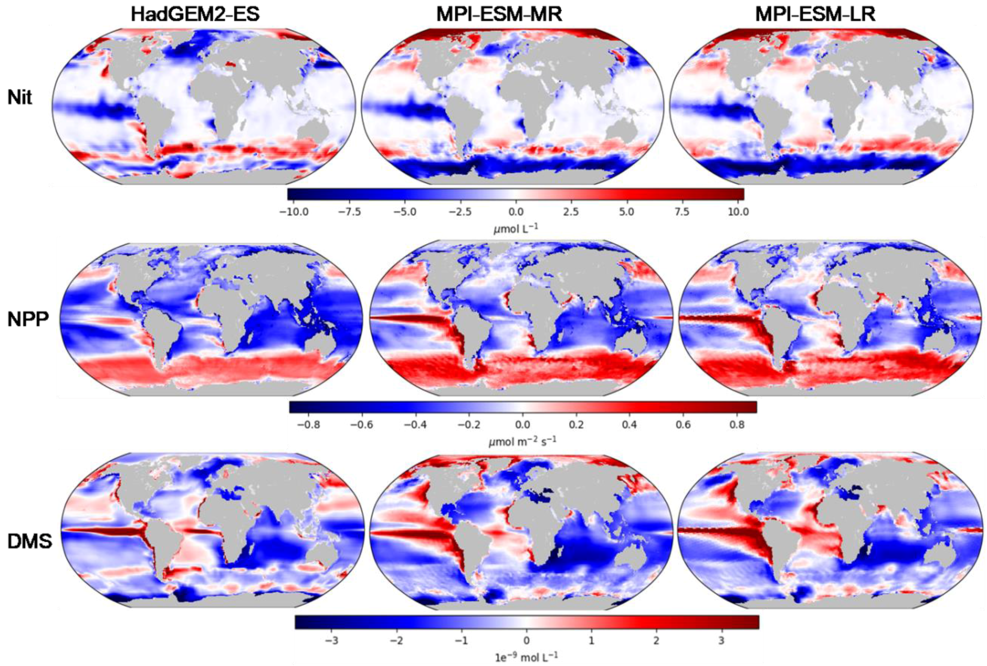
Uncertainties in nutrients will transfer through connecting biogeochemical processes to aerosol precursor emission, since the production of marine biogenic volatile organic compounds is strongly coupled to the underlying ecosystem. As expected, model-data benchmarking identifies areas of increased bias at high latitudes as well as in the tropical Pacific. Nutrient concentrations in the high-nutrient, low-chlorophyll (HNLC) region of the eastern tropical Pacific are lower in CMIP5 models when compared with World Ocean Atlas (WOA) datasets. Concentrations of nitrate, an essential macronutrient, are biased low by about 10 μmol L
−1 in the upwelling region (
Figure 2). The reduced concentrations of nutrients observed in these models suggest either weak vertical advection (mixing of nutrient-rich water) or a faster rate of consumption in the region. The availability of iron in this region will also play a part in regulating phytoplankton growth. Appropriate metrics to evaluate all of these issues will be strongly considered in the upcoming version of IOMB. Even with nitrate concentrations under-predicted in the tropical Pacific, net primary production is over-predicted by at least
in HadGEM2-ES, and greater than
in MPI models. Our results suggest that higher rates of carbon fixation in a given model could be responsible for the depletion of nitrate.
The positive excess in the rate of carbon fixation across upwelling regions of the tropical Pacific is also evident in the surface ocean DMS concentrations (
Figure 2). The tropical Pacific is of special interest because the environmental condition supports the constant production and flux of DMS. In the available observational dataset, the mean concentration of about 4 nM of DMS is maintained in the tropical Pacific throughout the year. This continual source of sulfur to the marine boundary layer provides natural equatorial sulfate that can be transported horizontally and vertically with the converging trade winds. The resulting aerosol moves poleward, and even into the stratosphere [
76]. Results for DMS surface ocean concentrations show a positive bias of almost a factor of 2 in the CMIP5 models. There is thus a possibility in the tropical Pacific of over-predicting the contribution of sulfate aerosol to cloud formation. This would lead to over-predicting of the equatorial albedo and cooling beyond observations.
Using IOMB, we estimate a total value of 30.6 Tg of sulfur transferred from the ocean into the MBL annually in the form of DMS gas. This is very close to the integrated value of 28.1 (17.6–34.4) Tg of S year
−1 provided for the same period in Lana et al. [
14]. The difference in global average emissions could well be traced back to the temperature field, which should affect the aqueous diffusion coefficient of the molecule. We also plan to investigate the diversity of the implied sea–air transfer schemes. DMS Computed Flux (DCF) for HadGEM-ES, MPI-ESM-MR and MPI-ESM-LR stand at individual levels of 21.1 Tg of S year
−1, 22.3 Tg of S year
−1, and 23.8 Tg of S year
−1 in IOMB. However, intrinsic fluxes from the various ESMs; which we refer to as the DMS Model Flux (DMF), predict higher emissions of 34.3 Tg of S year
−1, 39.2 Tg of S year
−1, and 42.3 Tg of S year
−1, respectively. Again, there will be the need to investigate other transfer mechanisms, along with biases in wind fields. It is also the case that at this early stage in the research, we have not yet considered in any direct way the cooling feedback effect of excess natural sulfur. This will generate considerable uncertainty in model outcomes through regional to global radiative forcing. What can be done working from the IOMB results presented here is to recommend regular marine aerosol checks, in order to place more realistic biogeochemical constraints on climate models.
The IOMB absolute scores in both DMF and DCF analyses are almost identical (
Figure 1), with DCF having a slightly higher absolute score due to the absence of atmospheric dynamics. Uncertainty in atmospheric processes represented in ESMs increases the overall DMS flux bias, the temporal bias, and RMSE, thus lowering the absolute score. Overall, DMF tropical Pacific sea-air flux rises to over
from about 8
, as estimated in the benchmark dataset (
Figure 3). For the HadGEM-ES model, the global period mean is
, with a bias of
. The positive bias reported in surface ocean DMS concentration propagates into the marine boundary layer with the models over-predicting the flux in the tropical Pacific and at high latitudes. Other than the regional offsets in the Greenland and Chukchi seas, simulations tend to match the referenced dataset within the Arctic circle. Predictions in the Southern Ocean were higher across all of the models by an average of
. Fluxes in the Weddell and Ross seas were slightly lower, but the high spatial bias in net primary production for this region suggests that representation of the haptophytes might be a contributing factor. This is also evidenced by the low model concentrations of DMS. The poleward shift of DMS distribution was mainly absent in the DCF benchmarking result, where fluxes match perfectly with the spatial trends in surface ocean concentration. This is due to the absence of atmospheric transport process.
The MPI-ESM model provides an opportunity to analyze the impact of spatial resolution in surface concentrations and sea-air fluxes. The IOMB variable scores for the two resolutions were similar except for silicate, which is an important nutrient for diatoms in making their hard exteriors. The most important disparity in silicate concentration lies in polar regions, where the lower resolution model shows a high silicate bias in the Norwegian Sea and the Weddell Sea relative to the WOA dataset. A significant depletion of Southern Ocean surface nitrate concentrations as a result of increased carbon fixation was more pronounced in these simulations than in the HadGEM model (
Figure 2). The period mean of surface ocean DMS concentrations, for the two MPI simulations, was
offset, and the average RMSE for this region was
. These two simulations give the same standard deviation from the concentrations benchmark dataset, but the mixed resolution simulation has a slightly lower correlation of 0.61. Warming and loss of Arctic sea ice and increasing biological activity in the open ocean led to higher DMS concentrations. As expected, this process is better represented in the high resolution simulation. By contrast, a high bias was more evident in the tropical Atlantic for the lower resolution configuration.
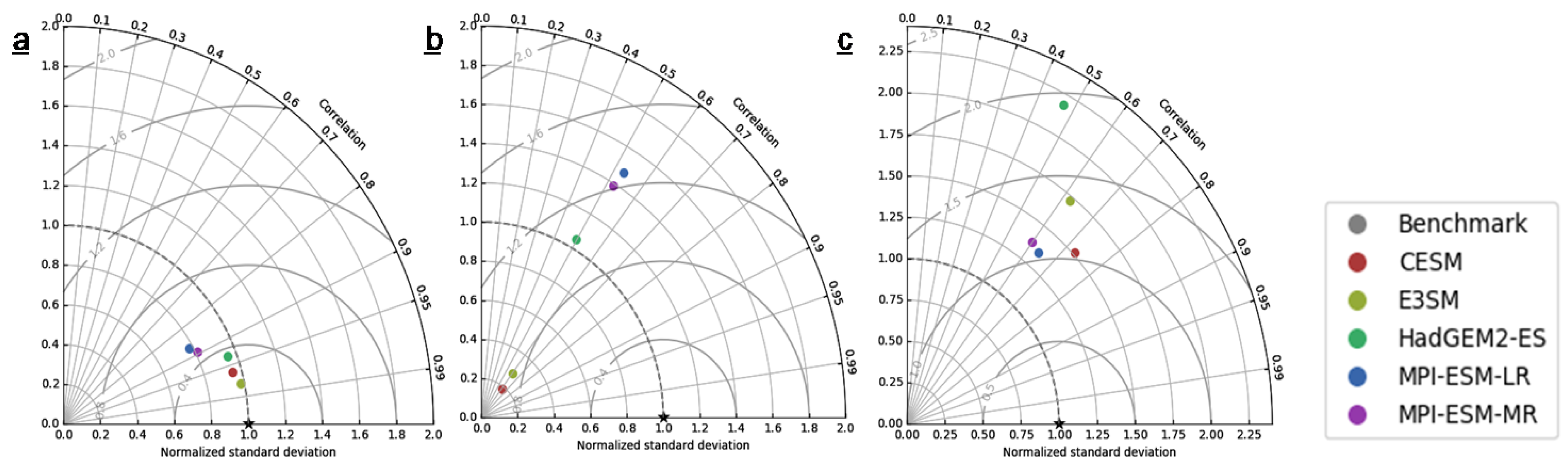
Overall, the results show increasing uncertainty as we progress through a list of biogeochemical processes. Derived products such as net primary production and DMS tend to have lower correlation and higher root mean square errors when compared with nutrients concentration in an ecosystem (
Figure 4). The uncertainty further increases as DMS enters the marine boundary layer. In contrast with the level of bias in surface ocean concentrations, DMS fluxes show higher uncertainties between models and the reference dataset. The whole Pacific Ocean, from the tropics all the way to the Bering Sea, displayed more DMS in the model results. This was also the case at the poles, as expected. Spatial correlation for areas below 45°S was about 0.78 for the three models, with HadGEM2-ES having the lowest RMSE of
, and MPI-ESM-LR having the highest at about
. The dynamics are different in the Indian Ocean, where DMS fluxes within the gyre dropped below what is obtainable in the referenced dataset.
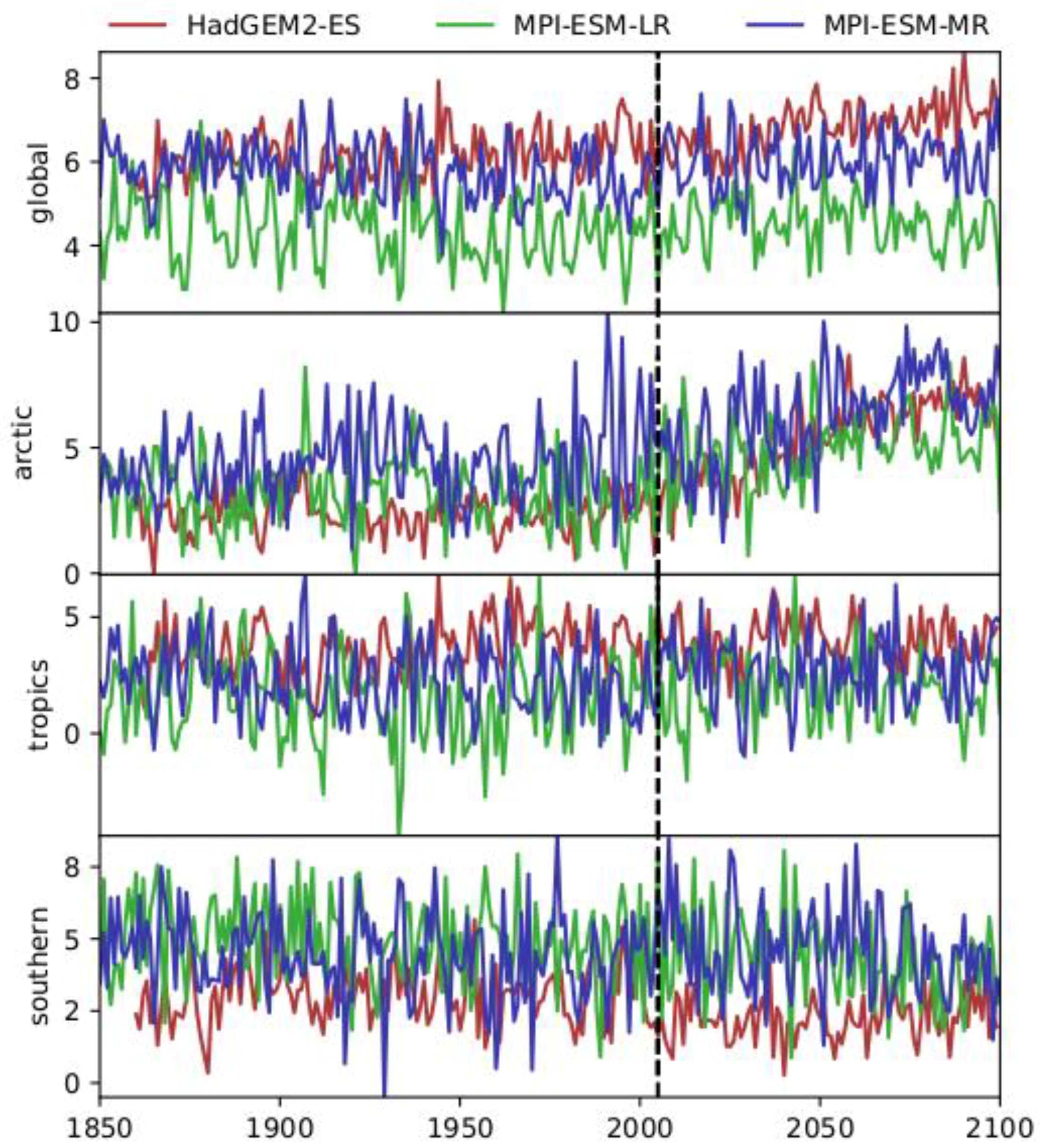
The uncertainty in surface ocean biogeochemistry and sea-air flux increases under Representative Concentration Pathway (RCP) 8.5 as the two CMIP5 models in this study tend to disagree on the direction of DMS flux on the global scale. HadGEM-ES projects a regional scale upswing of over
in the Arctic, leading to an overall increase in global mean by 2100 (
Figure 5). Global and regional trends have been fairly consistent since the industrial revolution; however, projection from the MPI models agree with a continuous DMS flux increase in Arctic open ocean as temperature increases. The connection between sea ice extent reduction, an increase in primary productivity, and a subsequent increase in marine biogenic aerosols, such as DMS, is more evident in the Arctic. However, the connection between sea-ice trends and aerosol precursor emissions is not definitive in the Southern Ocean. Results for the Southern Hemisphere show a gradual decline in the Southern Ocean flux going into 2100. Increases in global sea surface temperatures will ultimately have a dramatic impact on marine ecosystems, and may influence both primary productivity and the sea-air flux of marine aerosols. To determine the degree of influence of fundamental biogeochemical processes and validate future predictions, we continue to develop inherent metrics in IOMB.
4. Discussion
In the present work, we have outlined the importance of marine biogeochemistry to the generation of global aerosol precursors in the lower troposphere, and further to the determination of cloud structural feedback loops. The latter influences occur partly but not exclusively through the regulation of albedo over the ocean. We underscore the importance of incorporating the relevant processes in climate and Earth system simulations. Examples include, and we focused upon, the classic CLAW hypothesis, and volatile reduced sulfur sources [
4,
9]. However, we go further by noting that extensive validation must be supported if the new generation of models is to be successful. An automated framework is proposed and described based on the ILAMB package as a foundation and example [
10]. The marine version is now known as IOMB, which stands for International Ocean Model Benchmarking. The present paper constitutes one of the first descriptions of IOMB; its capabilities begin with standard nutrient-carbon cycling, as we demonstrate. However, we have intentionally incorporated the option to extend to the marine aerosol and related issues involving dissolved and volatile organics [
46,
56]. Benchmarking results with the global DMS database are presented and analyzed as examples of the need for further research, and here we venture to discuss the potential for future aerosol validation exercises.
Since the surface ocean is a major contributor of natural aerosol to the global troposphere [
3,
77], the sea necessarily acts as a point source for gases and particles, which become cloud condensation and ice nuclei. Microchemistry of the resulting aerosol distribution influences cloud reflectivity and lifetime across most of the planetary area [
11,
78]. Sulfate aerosols are of special interest, as high hygroscopicity and unique optical properties make them more suitable for cloud formation changes and increasing cloud lifetime. About 70% of natural sulfur emissions originate from the ocean as DMS. Our results show that approximately 30.6 Tg of sulfur get transferred into the atmosphere in a year. Tropospheric aerosol has contributed significantly to the moderation of global radiative forcing, which has been attributable to greenhouse gases since the industrial revolution [
21]. By contrast, with the long-lived heat trapping gases that prevent longwave radiation from escaping the top of the atmosphere, aerosol particles have exerted a net cooling effect operating primarily from below.
Accurate evaluation of the contribution of tropospheric aerosol to global radiative forcing requires a correct assessment of the natural contribution from marine sources. Although the parameterization of subgrid processes in contemporary ESMs has advanced over the decades, considerable regional biases still linger, from nutrient concentrations underlying the ecosystem to the mass of BVOCs released to the marine boundary layer. This is not unexpected, as layers of process complexity increase the uncertainty in simulated results. To reduce the degree of uncertainty associated with remote aerosols, marine biogeochemical simulations must be constrained with high quality observation datasets. All can agree that no ESM result will perfectly match observations, particularly across all temporal and spatial scales. However, well-defined and appropriately organized measurements clearly help to constrain model deviations. Biogeochemical simulation results within the accuracy bounds of their respective data serve to untangle the impacts of external forcings. Ultimately, this supports the quantification of secondary products such as the flux and concentrations of BVOCs as a class. Marine biogeochemical data providers are therefore encouraged to present the community with observational uncertainties, when available, in addition to raw values. Model skill can be better evaluated when benchmarked against data within the uncertainty bounds of the observation. It is unrealistic to expect system simulations to match specific values acquired on a restricted spatial scale.
The complexity of the marine aerosol benchmarking exercise stems partly from the ambiguities in the representation of the underlying global ecosystem within the ESMs. The corresponding atmospheric component of the model plays a strong role as well, and the associated uncertainties may be additive or antagonistic. However, in any case, a constructive effort to disentangle the subtleties begins with an objective benchmarking effort, which is focused specifically on marine biogeochemical processes. In coupled ESMs, over-prediction of the amount of natural sulfate originating from the ocean could create a false impression of increased sulfate aerosols and CCN. The resulting bias will necessarily offset global warming. Model intercomparison exercises show considerable deviation among participating groups. This challenges the reliability of at least some results. In light of this, a standard objective analysis against high quality observational datasets provides an enhanced level of fidelity and reliability.
We have performed our demonstrations here on dimethylsulfide distributions for three crucial reasons: (1) its natural aerosol feedbacks have been studied now for decades (CLAW), so that many thousands of insitu (analytical chemical) measurements have accumulated [
13,
14]; (2) organosulfur forms a logical starting point for the study of biogeochemical marine aerosol sources taken as a class [
2,
79]; and (3) as a methylated compound, DMS acts as a natural bridge to the next generation of modeling problems posed by dissolved organics as a whole. In fact, reduced sulfur processing highlights many of the most basic needs for the benchmarking of marine aerosol systems. Global biogeochemistry validation must soon extend in several new directions, and it is perhaps worth previewing them here at the level of discussion.
The DMS database itself continues to modernize. There are now algorithms available for the inversion of remotely sensed light fields to estimate concentration distributions [
33]. A certain amount of kinetics is involved, since relationships to the precursor dimethyl sulfonio-propionate (DMSP) are fundamental. The method is sufficiently new, so it may take considerable time to evolve toward fidelity; currently, the results are unpublished. However, it is possible that even the tens of thousands of determinations that have been analyzed by Lana et al. [
14] may soon prove to be just a starting point. The bulk of organic carbon released from phytoplankton does not contain sulfur as the major heteroatom [
12]. Most of the mass injected into the upper ocean water column is comprised of major components of the cytosol: proteins, polysaccharides, and lipids are most abundant. Some of the functionalities implied are extremely amphiphilic, and thus are surface active. The proteins and lipids must therefore participate directly in sea salt mass injections to the tropospheric boundary layer, with attendant regulatory effects [
2,
80,
81]. The latter take place through biomacromolecular adjustments to the distributed global marine surface tension [
3,
82]. As important as CLAW would seem to be, it can thus be argued that DMS is in fact merely one player among a host of organochemicals controlling marine particle injections.
The major surface-active macromolecules are biopolymeric, and hence they cannot enter the troposphere in the gas phase. However, they necessarily degrade through poorly understood channels into volatile compounds, with isoprene and the monoterpenes serving as major examples [
26,
83]. In all cases, measurements are not only less readily available than for our chosen starting point, the sulfide, but in fact they tend to be quite rare. The situation for the freshly released macromolecules was well reviewed in Ogunro et al. [
5]. Only a few hundred measurements have ever been reported, despite intimate relevance to the microlayer and aerosol systems. The terpene situation was well surveyed in Gantt et al. [
26], and it is only slightly superior. Plus, there is little hope of remote sensing coming to the rescue in these cases, considering that it may well have taken decades for even the CLAW hypothesis to attract real attention from the satellite community.
In such instances, there are several strategies that can be applied by our new benchmarking community. We can imitate methods from the early days of DMS study and extrapolate/interpolate according to marine biogeographic principals [
84,
85]. The methods have proven simple but effective, and include the radius of influence calculations bounded by ecological province definitions such that the arguments may apply across entire basins. In cases where hundreds of data points are distributed over the major biomes, it should be possible to construct reasonable first guess fields [
12,
13]. The OCEANFILMS’organospray parameterization has already begun using this method to predict adsorptive bubble-film sources of primary organics over the remote ocean [
86]. Complete Atlantic transects have recently appeared for both organic enrichment into the microlayer and (normalized) surface tension effects [
87,
88]. It should be possible to translate pole-to-pole latitudinal variation into a biogeographic viewpoint.
Additionally, since our primary interest is in connections running from ocean biogeochemistry to the global aerosol, IOMB should not neglect to enfold atmospheric microphysical and chemical data (above the sea–air interface). Organics have been mapped globally for their presence in fine particles for about a decade now [
15,
89]. Moreover, entire multiagency field campaigns are currently focusing on precisely the relationships that we propose to validate and benchmark (The North Atlantic Aerosols and Marine Ecosystems Study and Plankton Aerosol Cloud Ocean Ecosystem). An explosion of data is not at all unlikely, and this should be true both below and above the sea surface. New values should be adaptable biogeographically to become global scale datasets, beginning at the level of Kettle et al.’s [
13] type of interpolation-extrapolation. Validation will then drive fixes for several process structural omissions, which have proven difficult to rectify in marine systems modeling. The centrality of far upper ocean organic chemistry will be difficult to avoid in the face of a few key simulations and datasets. Recall that even given the full IOMB model population, many result suites are incomplete with regard to DMS (and therefore CLAW and most of planetary cloud albedo).
5. Conclusions
Marine biogeochemistry remains an important driving force for climate carbon-cycle feedback, as well as the production of aerosol particles in the MBL [
5,
6,
53]. There are numerous processes that link surface ocean biology with the composition of the lower atmosphere, such as the sea–air transfer of organic matter, ultimately serving as cloud or ice condensation nuclei and the release of organic macromolecules to become surfactants in the microlayer. The later influence salt spray production and gas exchange rates [
5,
80,
90]. Representation of these pathways in underlying biogeochemical routines within ESMs dictates the degree of uncertainty in the chemical composition, concentration, and oceanic emission rates of BVOCs, and the aerosol in general. To identify and reduce the discrepancies, we have developed an open source package that allows for objective data-model evaluation. We conclude that regional sensitivity in polar and tropical marine biogeochemical processes may constitute a major component of the uncertainty in MBL cloud representations.
The quantification of errors in MBL aerosol chemistry represents an extremely challenging task for the systems modeling community. This is true in large part because the required biogeochemical processes are currently less than well-represented in most contemporary ESMs. Some of the relevant physico-chemical mechanisms play out on a microscopic scale, so that subgrid parameterizations tend to be problematic on the global mesh. Regional models configured at finer resolution have done a better job of capturing the native dynamics that influence the production and transport of marine aerosols. For the immediate future, we envision rapid progress in the development of subgrid scale parameterizations for distributing and emitting aerosol precursors from the sea. The improvements will be data-driven, as high-quality observation sets are encoded appropriately in order to validate simulation outputs. The International Ocean Model Benchmarking or IOMB activity offers a novel, fully adaptable platform designed specifically for the necessary validation exercises. A wealth of marine physical and chemical processes can be examined independently, or in relation to atmospheric aerosol microphysical coupling.
Observational datasets available for benchmarking marine biogeochemistry are limited for logistical reasons that should be obvious: ship cruises are expensive and time-consuming. Similar arguments apply to aircraft campaigns. Remotely sensed data can be extremely convenient to use, but the suite of available variables is severely limited by optical and radiation transfer considerations. Although measurements and related compilations of ocean data have become more numerous and sophisticated in recent years, there is still much work to be done in the area of data collection and organization. Validation will constitute a centerpiece of the community effort as complex processes accumulate in the system codes. In the high-latitude case, a lack of data is even more conspicuous. Adverse weather conditions complicate sampling efforts, leading to restrictions on field campaigns. Profiling floats constitute a marvelous new tool kit, but they are expensive to initiate and operate, and even robotics bring with them certain geographical and temporal limitations. We anticipate that the community will push for improvements to remote sensing algorithms in order to further enhance their reliability—such as for example under cloud cover—and they may be extended to subtle variations on the standard theme of chlorophyll (pigment deconvolutions offering real biological resolution). Novel inversion methods may open up key chemical constituents to global mapping [
33]. At the same time, more ESMs involved in the ongoing CMIP exercise should be encouraged to output marine aerosol precursors such as DMS and related organics. Even as the various databases expand, benchmarking and analyses can only occur if the proper variables are simulated.
Overall, a benchmarking effort to quantify and reduce uncertainties in ESM simulation results can only be successful if the spatial and cumulative uncertainty in the observational dataset is appropriately reported. Results from global and regional models cannot perfectly overlap observations in all regions at all times, which is partly due to inherent uncertainties and unrepresented processes. However, models could be scored according to their skill set if the simulated result falls within the error range that is reported for the observation. Physical and biogeochemical variables can as a rule be benchmarked, along with other processes influencing the concentration of ocean-derived VOCs, their related materials, and their subsequent transfer into the MBL. The outcome will be improvements to subgrid parameterization and model development in order to capture the linkages in diagnostic simulations. Community capability to accurately represent natural contribution to the global aerosol forcing will be advanced. However, the identification of metrics that make appropriate use of observational data remains a scientific challenge. The spatial and temporal mismatch between models and measurements, biases in reanalysis and forcing data, model simplification, and structural and parametric uncertainties all contribute to the difficulty.
A major concern at this point is that the rate of global temperature rise might be faster than predicted in ESMs, because simulated surface ocean concentrations and emission rates of marine aerosols tend to be over-predicted. Models may possibly be providing more cloud cover and cloud albedo than the real atmosphere can produce. Marine sulfate aerosol could see little or no change in the tropics by the end of 20th century, but the extent of sea–air emissions may be lower than predicted. Increasing the primary productivity in the Arctic open ocean does suggest that there would be a continuous rise in DMS emission. Overall, CMIP5 models predict little to no change for the flux from the Southern Ocean, but there is limited agreement among the models on the amount of sea–air DMS flux from this region. The cloud droplet number concentration in the Southern Ocean is highly sensitivity to natural sulfate aerosol; thus, a large bias in ESMs’ representations of cloud radiative processes in this region could influence climate sensitivity projections. With a new release of IOMB scheduled soon, we continue to incorporate metrics and quality datasets that will allow us to quantify and reduce uncertainty in climate carbon-cycle feedbacks and marine MBL cloud systems.

 ,
, 


