A Simulation Study of Global Evapotranspiration Components Using the Community Land Model


1
College of Meteorology and Oceanography, National University of Defense Technology, Nanjing 211101, China
2
Nanjing Star-jelly Environmental Consultants Co. Ltd., Nanjing 210013, China
*
Author to whom correspondence should be addressed.
Atmosphere 2018, 9(5), 178; https://doi.org/10.3390/atmos9050178
Submission received: 6 March 2018
/
Revised: 20 April 2018
/
Accepted: 4 May 2018
/
Published: 8 May 2018
(This article belongs to the Section Biosphere/Hydrosphere/Land–Atmosphere Interactions)
Abstract
:The Qian atmospheric forcing dataset is used to drive the Community Land Model, version 4.0 and 4.5 (CLM4 and CLM4.5) in off-line simulation tests. Based on flux network (FLUXNET) data and reanalysis data provided by National Oceanic and Atmospheric Administration (NOAA) and Climate Forecast System Reanalysis (CFSR), the simulation results of CLM4.5 on the global evaporation of intercepted water from the vegetation canopy (Ec), vegetation transpiration (Et), evaporation of soil (Es) and latent heat flux are evaluated. Subsequently, the improvement in the simulation results of CLM4.5 compared with CLM4.0 is tested and analyzed. The results show that the simulated spatial distribution of Ec, Et and latent heat flux in CLM4.5 are closer to the reanalysis data than Es. The simulated annual means of Et, Es and latent heat flux in CLM4.5 are larger than the reanalysis data, but Ec is smaller. The spatial distribution of the simulation bias of latent heat flux in CLM4.5 is mainly determined by the bias distribution of Es. There is a significant difference in the simulation of Et, Es and latent heat flux between CLM4.5 and CLM4.0. These differences are mainly present near the equator and in the middle and high latitudes in the Northern Hemisphere. In general, compared with CLM4.0, the simulation bias of Et, Es, and latent heat flux have been reduced in CLM4.5, and the simulated means are more consistent with the reanalysis data. Although there is a significant improvement in the simulation of the spatial distribution of Et and Es in CLM4.5 compared with CLM4.0, the ability of CLM4.5 to simulate the spatial distribution of global latent heat flux shows little improvement relative to CLM4.0.
1. Introduction
Evapotranspiration (ET) refers to the loss of water from land surfaces into the atmosphere through the evaporation of soil (Es), the evaporation of intercepted water from the vegetation canopy (Ec), and vegetation transpiration (Et). Approximately 60% of surface precipitation returns to the atmosphere in the form of ET; this quantity can reach more than 90% in arid areas [1]. The energy formed by ET is called latent heat flux. Half of the solar radiation absorbed at the earth’s surface is consumed through ET [2]. ET is an important component of the land surface energy balance and the water budget and plays a key role in weather and climate systems as well as the hydrological cycle [3]. ET is also a key parameter for studying climate change and land surface processes. Studies have shown that the intensity and duration of ET can strongly affect weather and land surface processes, carbon and nitrogen cycles in ecosystems, surface albedo, ground temperature, fluvial flow, and groundwater recharge [4,5,6]. ET plays an important role in the soil-vegetation-atmosphere system, and ET has always been one of the most difficult physical quantities to directly measure in hydrological cycles. It is very important to understand the distribution of ET at different temporal and spatial scales to accurately estimate the effects of ET on weather, climate, and ecosystems for environmental assessments and the management of water resources.
Currently, the research methods for ET mainly use remote sensing technology and land surface models. Remote sensing technology is primarily based on the surface energy balance model and a conventional method combined with an empirical formula (i.e., the Penman-Monteith formula) [7,8,9]. However, previous studies have shown that ET obtained through remote sensing creates more uncertainty than land surface models, in cases where the available time scale was also limited [10]. In the use of land surface models, Lawrence et al. [11] used the CLM3.0 model to carry out a simulation study on the distribution proportion of the components of evapotranspiration at the global scale, and a series of improvements were made to enhance the simulation performance of the model. Schlosser and Gao [12] estimated global ET using the simulation data of 13 land surface models from the second Global Soil Wetness Project (GSWP-2). They found that the sensitivity of the models to atmospheric forcing data was weaker at the global scale, and the interannual variability in high latitude regions and the seasonal variability in tropical regions varied greatly between the models. Wang and Dickinson [13] reviewed observations and research for global land ET. Sun et al. [10] used multiple land surface models (CLM4.0, Dynamic Land Model (DLM) and Variable Infiltration Capacity model (VIC)) to assess the temporal and spatial variability of ET in China from 1979 to 2012. Since the response time scales between the components of ET and the atmosphere are different (Ec is the fastest, followed by Es, with Et being slowest), the interaction between ET and the local climate is likely to be affected by the proportional distribution of ET from each of its components [11]. Therefore, it is necessary to study the components of evapotranspiration.
The CLM is one of the most widely used land surface models in the world [14]. Some scholars have improved the parameterization schemes for some components of ET in CLM4.0 [15]. In particular, Bonan et al. [16] improved simulations for vegetation canopy radiation, photosynthesis processes and related parameters to improve the simulation of gross primary productivity (GPP) and latent heat fluxes (especially Et). Sun et al. [17] used a new Newton-Raphson iteration scheme to address coupling photosynthesis rates and stomatal conductance and reduced the simulated bias of Et caused by iteration non-convergence. Swenson et al. [18] improved the hydraulic properties of soil in permafrost regions and improved the model’s ability to simulate soil moisture. Although these improvements achieved good results and became part of the CLM4.5 parameterization, due to the interaction between the ET components (i.e., the water required for the Et comes from soil, therefore, Et and Es interact with each other), the resulting improvement in CLM4.5 in comparison with CLM4.0 with regard to ET components and latent heat flux was not analyzed. Therefore, some scholars still choose CLM4.0, rather than CLM4.5, to study ET [10,19].
In this paper, we will use CLM4.5 and CLM4.0 for offline simulation tests to evaluate the performance of CLM4.5 on simulating Ec, Et, Es and latent heat flux compared with FLUXNET data [20,21] and reanalysis data provided by National Oceanic and Atmospheric Administration (NOAA) [22] and Climate Forecast System Reanalysis (CFSR) [23] in the form of energy. In addition, to compare different versions of CLM and to provide a reference for further model improvement, another objective of this study is to test and analyze CLM4.5 relative to CLM4.0 in terms of improvements to the analysis of Et, Es, and latent heat flux. In the following, Section 2 includes a brief description of CLM4.5, experiment design, and data. Section 3 presents the results analysis. The conclusion and discussion are given in Section 4.
2. Methods
2.1. Brief Model Introduction
The CLM land surface model series is a global dynamic land surface simulation system developed primarily by the National Center for Atmospheric Research (NCAR) based on the Community Earth System Model (CESM) framework program. CLM integrates the advantages of several land surface models, such as the Biosphere-Atmosphere Transfer Scheme (BATS) [24], the 1994 version land surface model of the Chinese Academy of Sciences Institute of Atmospheric Physics (IAP94) [25], and Bonan's Land Surface Model (LSM) and has become one of the most developed and promising land surface models in the world. It has been coupled with the CCSM climate model, CESM earth system model, mesoscale models (such as WRF), and regional climate models (such as RegCM). CLM4.5 is the land surface component of the new version of CESM1.2 released by NCAR. CLM4.5 contains 15 layers of soil that are in total 42.1 m deep, but only 10 layers (down to 3.8 m) are hydrologically active with soil properties. The bottom five layers have bedrock properties. The soil is divided into 20 categories, and plant functional types (PFT) are divided into 17 categories. Fang et al. [14] gave a detailed description of the differences between CLM4.5 and CLM4.0.
2.2. Experiment Scheme and Data
In this paper, CLM4.0 and CLM4.5 performed offline simulations for the years between 1952 and 2002 using the satellite phenology option, where the years 19521–982 were used for the spin-up. Land cover was held constant at values for the year 2000. The Qian dataset [26], which combines NCEP–NCAR reanalysis data and observation-based analyses of monthly precipitation, surface air temperature, and surface downward solar radiation, was used as the atmospheric forcing data. This dataset was extensively applied to the improvement and evaluation of the land surface model [16,17,27,28,29,30,31,32]. The spatial resolution of the model is 1.25° in longitude by 0.9375° in latitude. The vegetation reanalysis data (Ec and Et) were provided by NOAA [22]. The reanalysis data for Es and latent heat flux were provided by CFSR [23] and FLUXNET data [20,21] respectively. The distribution of PFT based on remote sensing data (see Figure 1) and the leaf area index (LAI) and stem area index (SAI) for vegetation based on satellite phenology data that takes monthly variation into account (see Figure 2) and were provided by the Moderate Resolution Imaging Spectroradiometer (MODIS). It is worth mentioning that the unit of Ec and Et provided by NOAA and Es provided by CFSR are in W/m2. For the convenience of comparing, latent heat flux and its components are presented in terms of energy (W/m2) instead of water flux (mm) in this article.
3. Results Analysis
3.1. Canopy Interception Evaporation
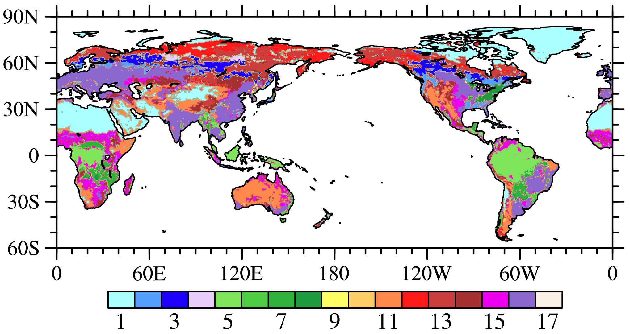
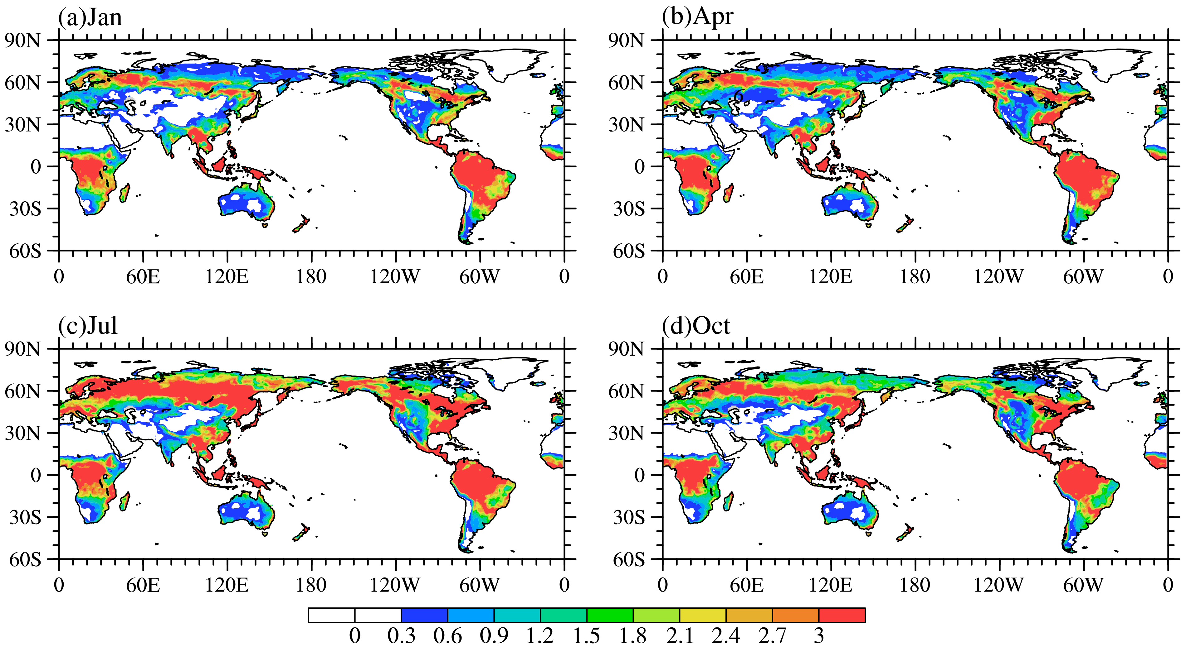
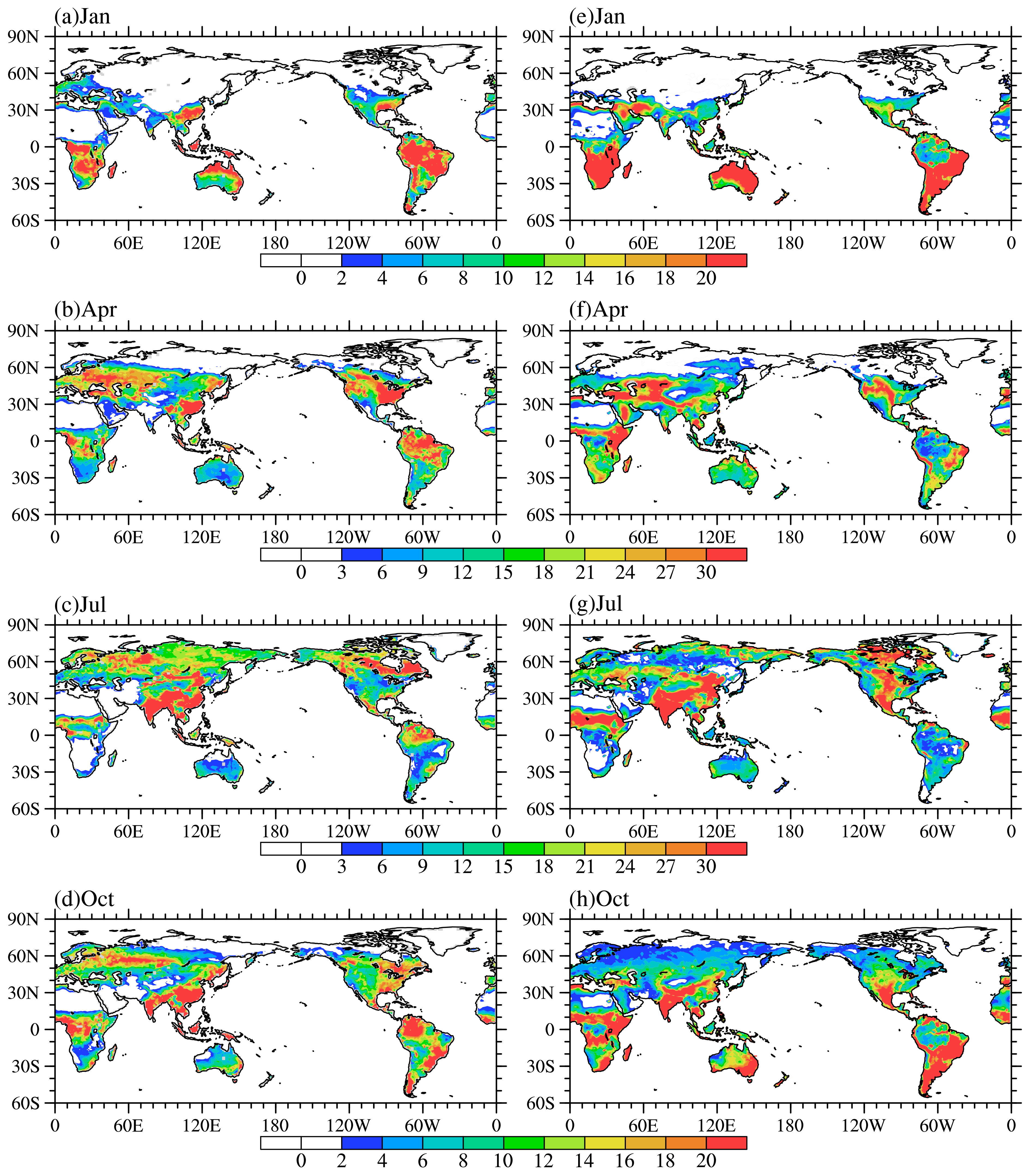
In Figure 3, the seasonality spatial pattern of global Ec is given from the simulation results of CLM4.5 and the reanalysis data. From the reanalysis data shown in Figure 3a–d, global Ec presents zonal distribution characteristics and seasonal variation. Ec is mainly present in the Southern Hemisphere in January; in July, it is mainly present in the Northern Hemisphere; and in April and October, it decreases moving from the equator to the poles. Figure 4 shows the seasonal distribution of global precipitation derived from Qian atmospheric forcing data, and it can be seen from Figure 2 and Figure 4 that the seasonal variation of the spatial pattern of Ec is determined by the seasonal variation of the spatial pattern of precipitation and the sum of LAI and SAI. In terms of climate type, the large values of Ec are mainly concentrated in the tropical rainforest and tropical monsoon climate zones. When we calculate the annual average of Ec between 15° S and 15° N from the reanalysis data, we find that Ec in this area account for 46.1% of the global total. It can be seen from Figure 1 that the tropical broad-leaved forest is the dominant vegetation type in that area, and the sum of LAI and SAI is relatively large (see Figure 2), which results in the stronger interception capacity of canopies in these areas. In addition, these areas have abundant water vapors (see Figure 4). Therefore, the combined effects of sufficient precipitation and the strong interception ability make Ec in these areas larger than that of other regions. However, in some desert areas (e.g., northern Africa, the Middle East Peninsula, Central Eurasia, and South-Western Australia), polar regions (e.g., Greenland and northeast Canada), glaciers and permafrost regions (e.g., the Rocky Mountains, the Andes and the Tibetan Plateau), Ec is relatively small. This is because the vegetation types in these areas are mostly non-vegetation, shrubs and cold grasslands. Vegetation coverage is low, and the surface roughness is relatively small, which is not conducive to the flux of water vapor. The surface albedo is also large, so the temperature of sinking air flow increases and compensates for energy loss at the ground [33]. As a result, in these areas, there is less precipitation and a weaker canopy interception capacity, so Ec is relatively lower than the other regions. As observed from Figure 3e–h, the simulation results of seasonal variation and distribution characteristics of Ec in CLM4.5 are consistent with the reanalysis data. The annual average of Ec between 15° S and 15° N is also calculated and is found to account for 58.5% of the total global Ec, which is larger than the amount found in the reanalysis data (46.1%).
We use CLM4.5 as the representative model because CLM4.5 and CLM4.0 have the same canopy interception parameterized scheme and, therefore, the simulated results in both models are almost identical. Table 1 shows the root mean square errors (RMSEs), means and spatial correlation coefficients of the simulated results of CLM4.5 and the reanalysis data of the global Ec. From Table 1, we can see that the spatial correlation coefficients of simulated results and the reanalysis data in January, April, July and October and the annual average are 0.91, 0.91, 0.85, 0.89 and 0.90, respectively, indicating that the model has a relatively strong ability to simulate the spatial distribution of Ec in January and April. However, compared with the reanalysis data, the simulated mean of Ec is relatively small, especially in July, and the RMSE is large, which indicates that there may be a systematic weakness in the simulation of Ec in CLM4.5. Figure 5 shows the seasonal distribution of the difference of Ec between the simulated results of CLM4.5 and reanalysis data. It can be seen from Figure 5 that, except for southwestern Eurasia, Greenland, northern Australia, part of South America, and the high latitude region of the northern hemisphere in April, the simulated Ec is smaller than the reanalysis data over much of the globe.
Through the analysis of the canopy interception parameterization scheme, the findings indicate that the physical variables related to the canopy interception process (e.g., throughfall, canopy drip) are considered in the model design principle [15]. However, the existing interception calculations do not directly consider the influence of rainfall intensities and wind speeds. For example, when raindrops reach the leaf surface at a certain speed, splash droplet evaporation (SDE) is produced. Similar research findings propose that rainfall intensity plays a decisive role in the process of canopy interception and evaporation and that 10–40% of precipitation will be consumed in the process of SDE under heavy rainfall [34,35]. Wind can influence canopy interception precipitation by shaking branches [36,37,38,39]. Besides, an interception by vegetation does not distinguish between liquid and solid phases, namely rain and snow are treated the same, which may have an influence on Ec in the middle and high latitudes in winter. These factors may act as the possible causes of the canopy interception simulation bias. Therefore, accounting for these factors is one possible path to further improve the model.
3.2. Vegetation Transpiration
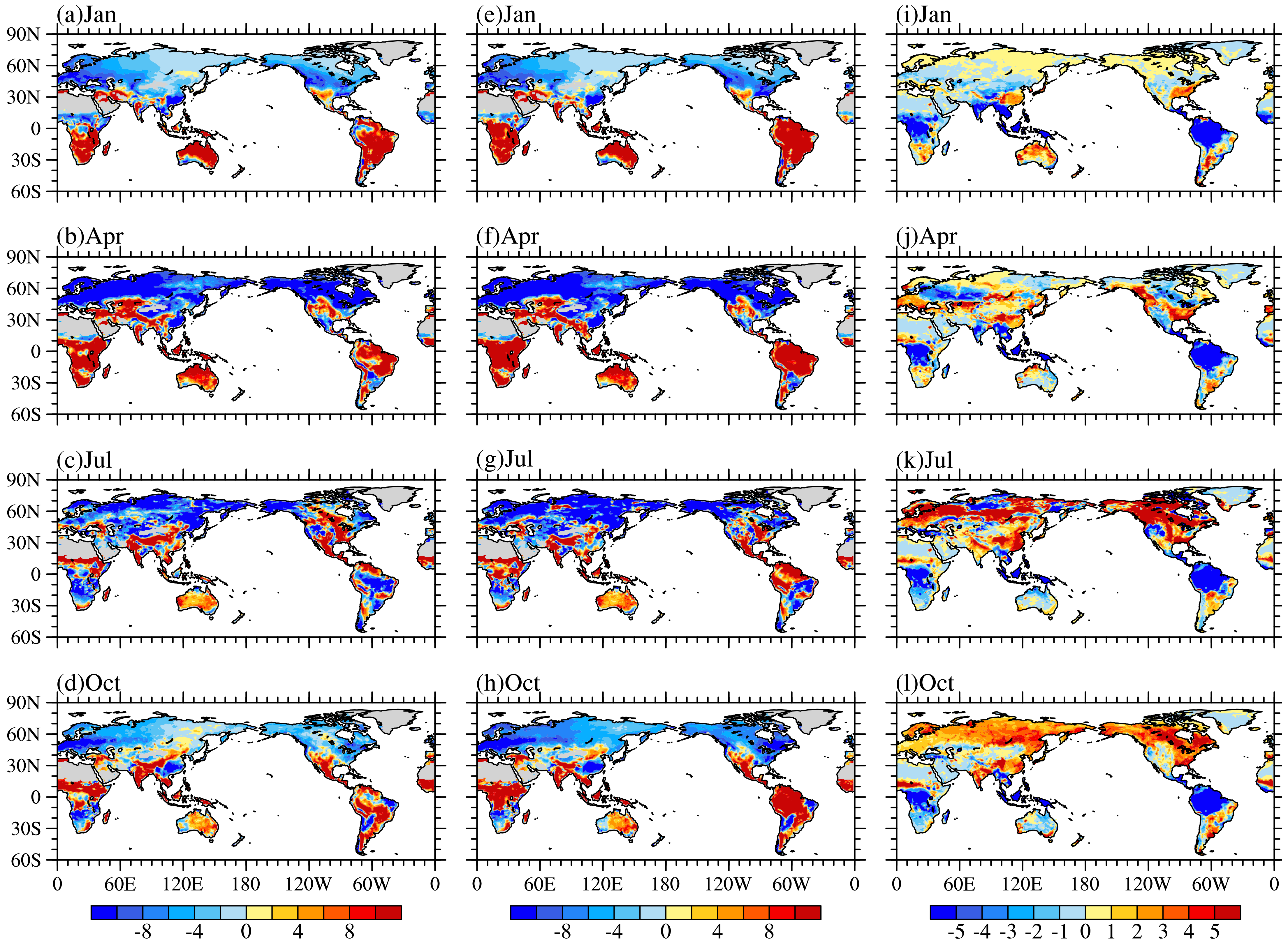
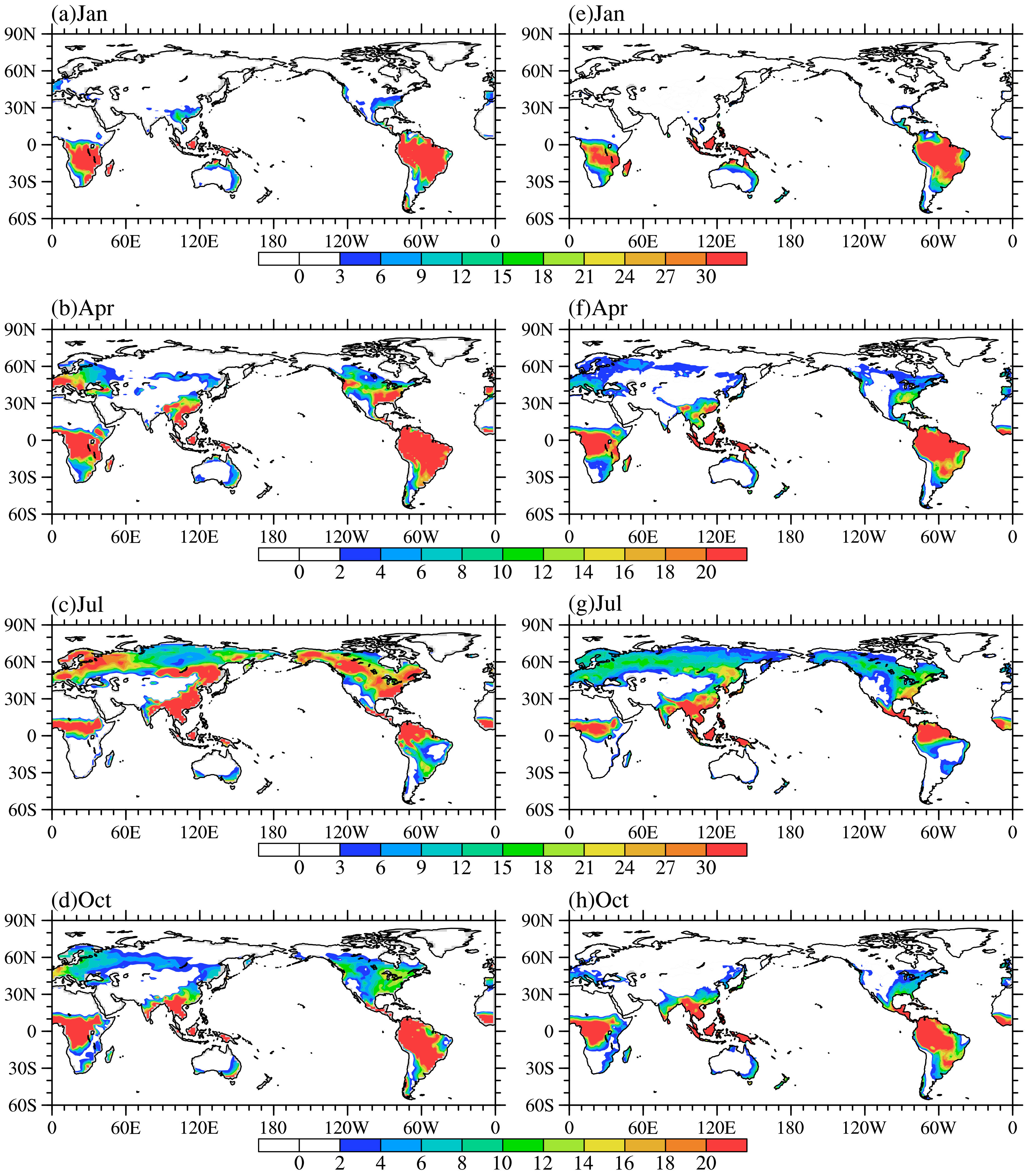
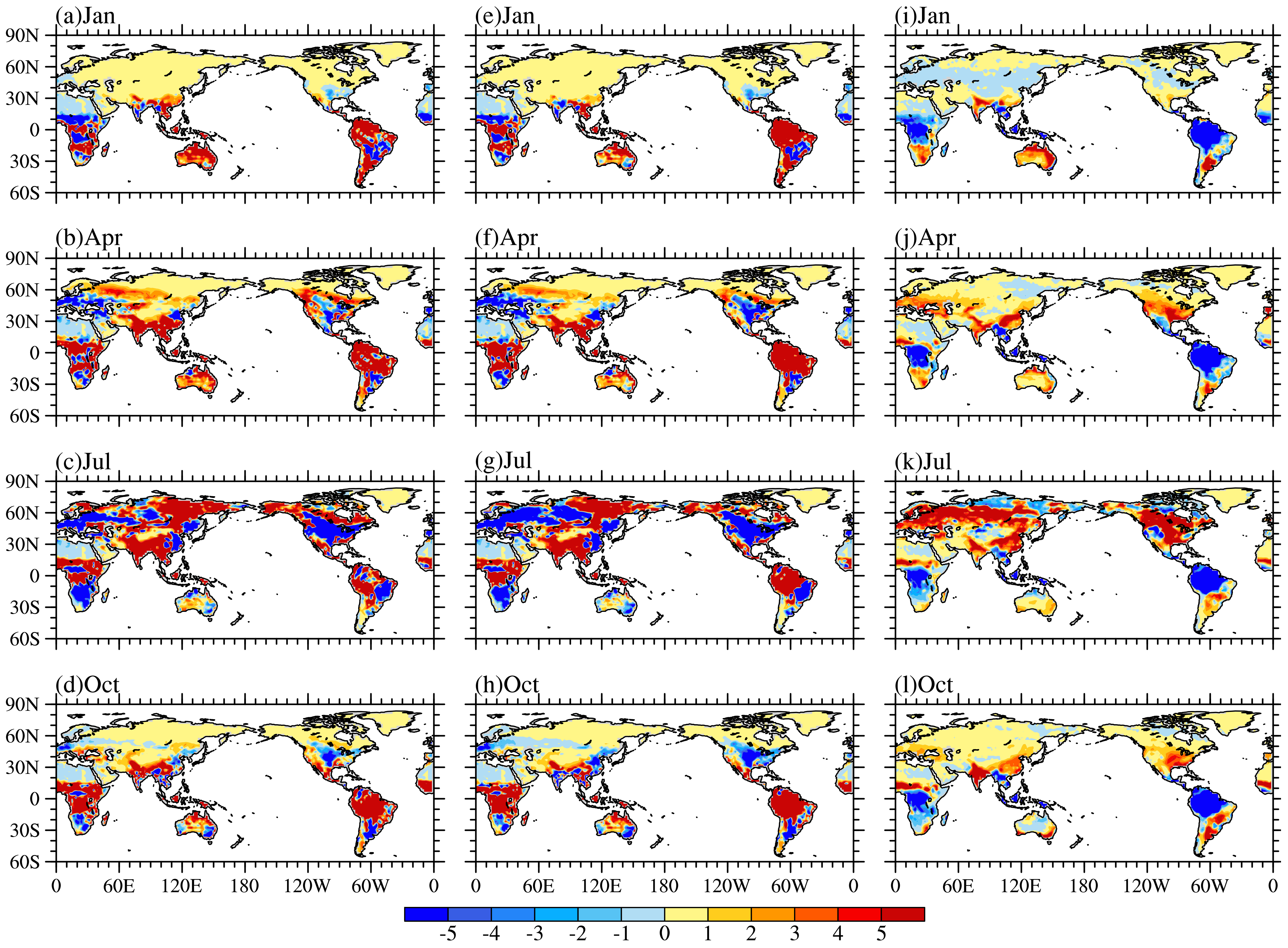
Figure 6 shows the seasonal spatial pattern of the simulation results of CLM4.5 and the reanalysis data of global Et. As observed from Figure 6a–d, similar to Ec, Et also has obvious seasonal variations. Et is concentrated in southern Africa and southeastern Latin America in January, and in the Northern Hemisphere, Et increases gradually in April in Europe, Southeast Asia and southern North America and reaches its maximum in July with Et mainly concentrated in the Northern Hemisphere. Et concentration then gradually moves toward the Southern Hemisphere in October. As observed from Figure 6e–h, the model effectively simulates the seasonal variation of Et and the distribution of high and low value centers. Table 2 shows the RMSEs, means and spatial correlation coefficients of the simulation results of CLM4.5 and reanalysis data of the global Et. Table 2 demonstrates that spatial correlation coefficients of the simulated results of CLM4.5 and the reanalysis data are approximately 0.89, indicating that the simulated spatial distribution in CLM4.5 is close to the reanalysis data. Additionally, it can be observed from Table 2 that the simulation results of CLM4.5 on Et are relatively larger than that of the reanalysis data. Figure 7 shows the differences among the reanalysis data, CLM4.5 and CLM4.0. As observed from Figure 7a–d, the simulated Et in CLM4.5 is relatively large in most areas compared with the reanalysis, and the bias between the models is especially concentrated near the equator and South Asia.
Due to the work of Bonan et al. [16], Sun et al. [17] and Swenson et al. [18], the simulation results of CLM4.5 and CLM4.0 on vegetation transpiration were significantly different (see Figure 7i–l). Comparing Figure 7e–h with i-l, CLM4.5 has clearly reduced the simulation bias in CLM4.0, and the spatial correlation coefficients in January, April, July and October are −0.54, −0.67, −0.53 and −0.71, respectively. As seen from Table 2, the RMSEs of CLM4.5 are clearly smaller than those of CLM4.0. Although the simulation result of Et from CLM4.5 is larger than that of CLM4.0 in the middle and high latitudes in July, which produces a large simulation bias for the mean, it is encouraging that the simulated means in CLM4.5 in January, April and October are closer to the reanalysis data. The reason is that Bonan et al. [16] had improved the leaf parameterization process, which changed the stomatal conductance, and resulted in the limitation of photosynthesis, especially in the equatorial region, and this improvement significantly reduced the simulated mean of Et in CLM4.0. Swenson et al. [18] found that dry soil biases result from the CLM4.0’s formulation of soil hydraulic permeability when soil ice is present and excessively dry soils in permafrost regions. By correcting the parameterization of the hydraulic properties of the frozen soil, the simulated moisture contents in the near-surface is more accurate. As the water required for Et is derived from soil, Swenson et al. [18] found the Et in the middle and high latitudes of the Northern Hemisphere to be relatively larger than that of CLM4.0. Sun et al. [17] discovered that iterative calculation of transpiration does not converge in large portions of land surface in CLM4.0 by using a fixed-point iteration approach. They proposed that a new approach, the Newton-Raphson iteration, can ensure convergence without requiring an artificial constraint. The differences between CLM4.5 and CLM4.0 in parts of India, Australia, North America, and Eurasia may be explained by the work of Sun et al. [17].
Table 3 shows the annual mean of Et of the main PFTs in CLM4.0 and CLM4.5 and their differences. It is worth noting that for the main PFTs, only the Et of the 5th kind of PFT (tropical evergreen broad-leaved forest near the equator) simulated by CLM4.5 is smaller than that of CLM4.0. The reason for why the simulated Et in CLM4.5 is smaller than that in CLM4.0 in the equatorial region, is primarily due to the reduction of Et in tropical evergreen broad-leaved forests, which shows that the model improvement work of Bonan et al. [16] is well reflected in CLM4.5, based on the analysis on Et.
3.3. Soil Evaporation
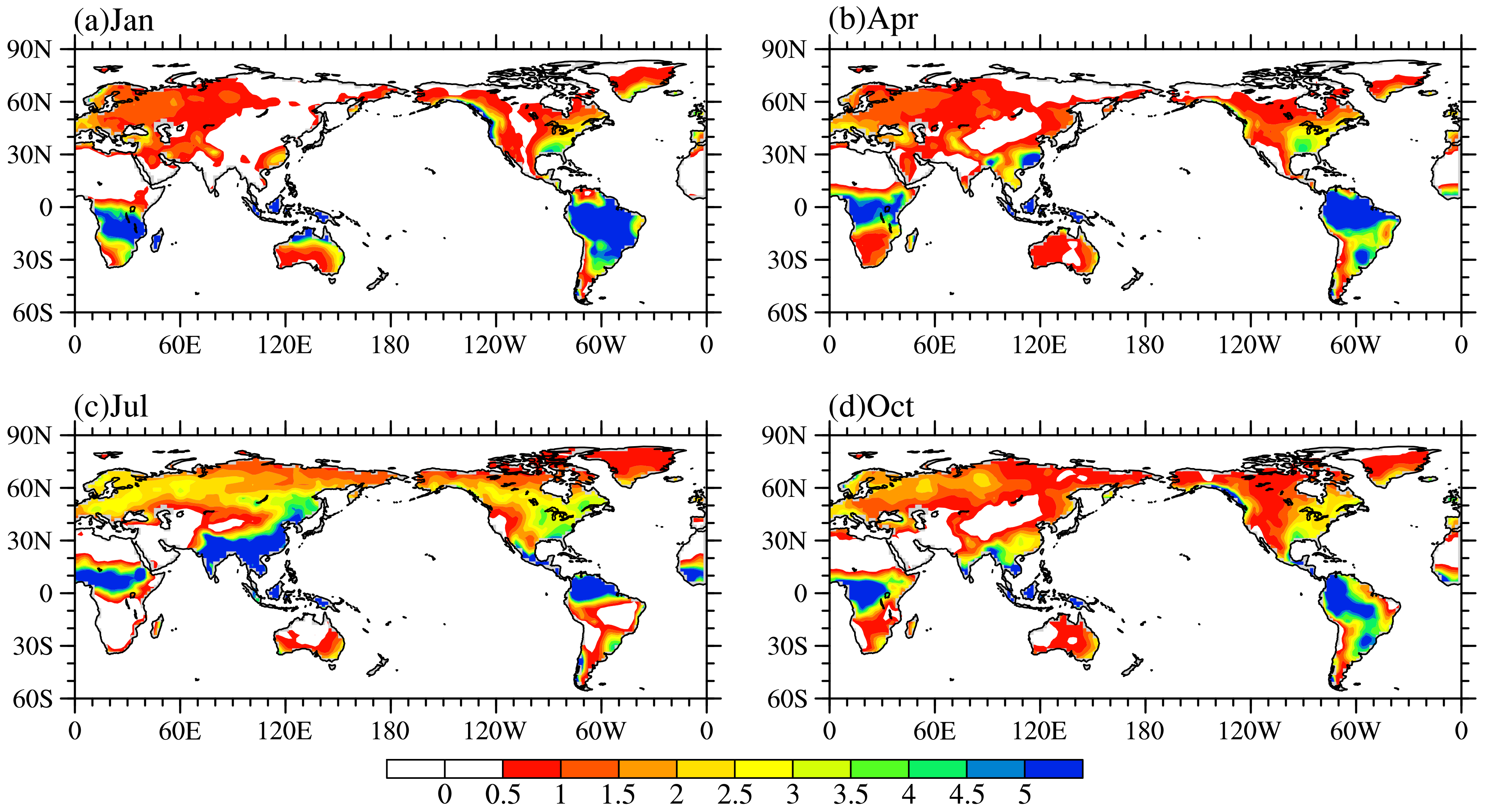
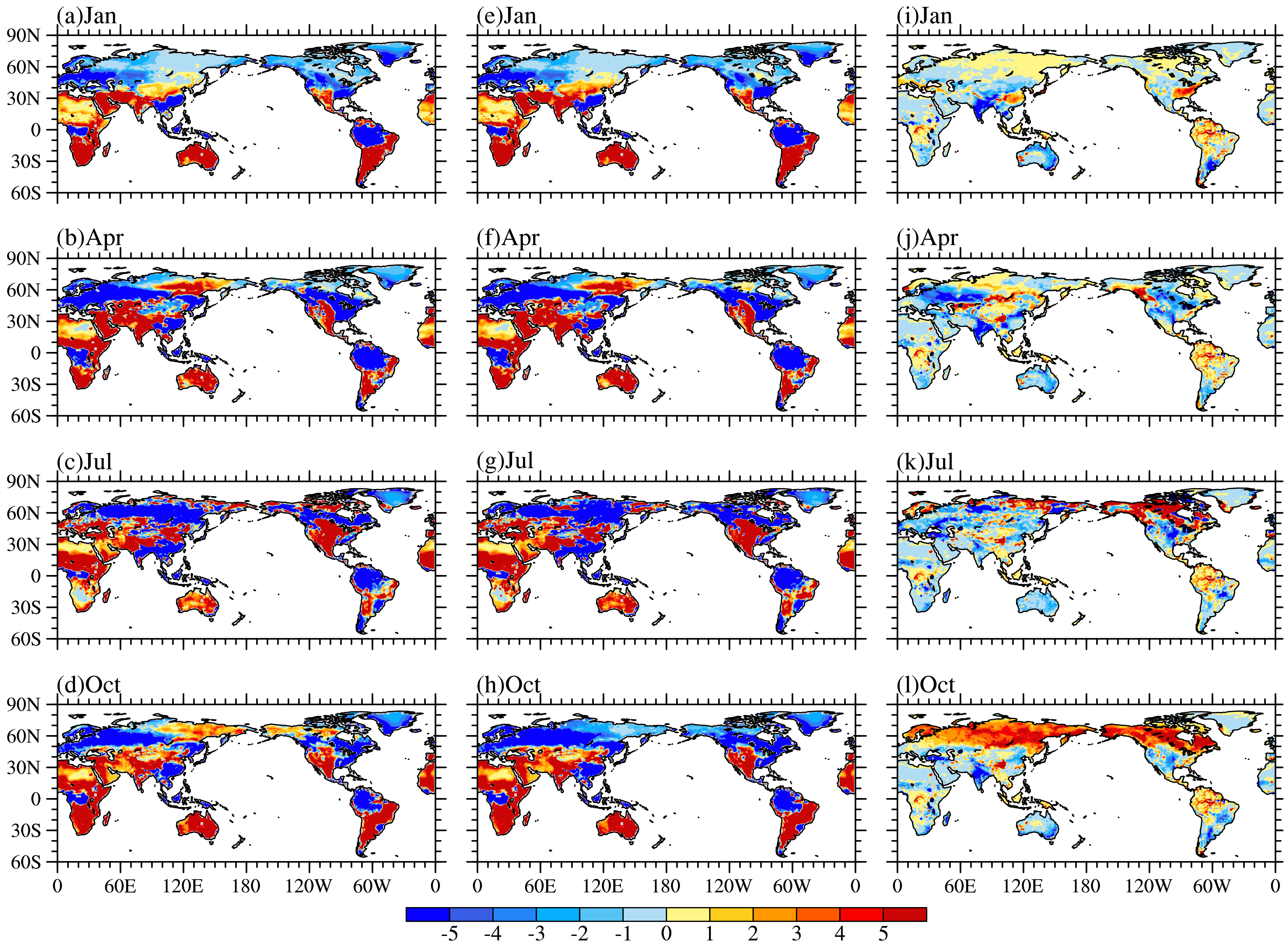
Figure 8 shows the seasonal spatial patterns of the simulation results of CLM4.5 and the reanalysis data of global Es. As observed from Figure 8, CLM4.5 effectively simulates the seasonal variation of Es, but there is a large difference in the distribution of the high and low values between the simulation results of CLM4.5 and the reanalyzed data. Table 4 shows the RMSEs, means and spatial correlation coefficients of the simulated results of CLM4.5, and reanalysis data of global Es. From Table 4, it can be observed that the spatial correlation coefficients of the simulated Es in CLM4.5 and the reanalysis data in January, April, July, October, and annual average are 0.64, 0.52, 0.58, 0.53 and 0.53, respectively, which is smaller than that of Ec and Et, indicating that there are major differences in the spatial distribution of global Es between CLM4.5 and the reanalyzed data. Figure 9 shows the differences among the reanalysis data, CLM4.5, and CLM4.0. As observed from Figure 9a–d, the simulation results of CLM4.5 on Es in equatorial regions are significantly lower in comparison to the reanalysis data, which may be caused by the strong Et in those regions (see Figure 7a–d). The Es in most areas of the middle and high latitudes in the Northern Hemisphere is relatively low in January and July, while it is generally high in the southwest of Asia, southwest North America, northern Africa and most parts of the Southern Hemisphere. As seen from Table 4, the simulated means of Es in CLM4.5 in January, July and October are larger than the means in the reanalysis, and the mean of Es is smaller in April. The simulated mean in October (7.0 W/m2) is very close to the reanalysis data (6.9 W/m2), indicating that CLM4.5 has a relatively strong simulation ability for the mean of Es in October.
From Figure 9i–l, it can be observed that the simulated Es in CLM4.5 is larger than that of CLM4.0 near the equator because the transpiration capacity of CLM4.5 is limited in the equatorial region. The bias distributions in Figure 9i–l and Figure 7i–l are opposite of one another in most areas, especially in the Southern Hemisphere, which reflects the close relationship between Es and Et. That is, when the vegetation transpiration increases the soil moisture coefficient, the difference in humidity between the reference height and ground surface will decrease, resulting in a decrease in soil evaporation [15]. The error distributions of Figure 9e–h and Figure 9i–l are also basically the opposite of one another. From Table 4, we can see that the spatial correlation coefficients between CLM4.5 and the reanalysis data are larger than that of CLM4.0, and the RMSEs are relatively small. In addition to April, the simulation results of CLM4.5 of the means are closer to the reanalysis data than CLM4.0. In general, the ability of CLM4.5 to simulate soil evaporation has been significantly improved when compared with CLM4.0.
Although the simulated soil moisture in CLM4.5 is larger than that of CLM4.0 in the middle and high latitudes in the Northern Hemisphere (figure omitted), the enhanced Et in CLM4.5 in that region in April and July does not increase Es. Even if Et slightly changes in January and October in the middle and high latitudes in the Northern Hemisphere, the Es in January is suppressed due to the snow cover, resulting in a significant increase in the Es of CLM4.5 compared to CLM4.0, but only in October.
3.4. Latent Heat Flux
Figure 10 shows the seasonal spatial pattern of the simulation results of CLM4.5 and the reanalysis data of global latent heat flux. From Figure 10, it can be seen that CLM4.5 can effectively simulate the seasonal variation and the center position of the high and low values of the latent heat flux. Table 5 shows the RMSEs, means and spatial correlation coefficients of the simulated results of CLM4.5, and reanalysis data of the global latent heat flux. From Table 5, we can see that the spatial correlation coefficients of the simulated results of CLM4.5 and the reanalysis data in January, April, July and October and the annual average are 0.97, 0.92, 0.88, 0.96 and 0.91, respectively. This indicates that CLM4.5 has relatively strong simulation ability for global latent heat flux spatial distribution in January and October. In addition, the simulated means of latent heat flux in CLM4.5 are relatively larger than those of the reanalysis data. Figure 11 shows the differences among the reanalysis data, CLM4.5 and CLM4.0. As seen from Figure 11a–d, the negative bias is primarily concentrated in the middle and high latitudes in the Northern Hemisphere, while the Southern Hemisphere is dominated by positive bias. The spatial correlation coefficients between the bias distribution of global latent heat flux and Et calculated by the difference between the simulation results of CLM4.5 and the reanalysis data (see Figure 11a–d and Figure 7a–d) in January, April, July and October are 0.38, 0.36, 0.18 and 0.41, respectively, but the spatial correlation coefficients between the bias distribution of global latent heat flux and Es (see Figure 11a–d and Figure 9a–d) for the same months are 0.69, 0.66, 0.53 and 0.54, respectively. These data indicate that the bias distribution of latent heat flux is primarily determined by the bias distribution of Es, in which reducing the simulation bias of Es can be helpful in improving the simulation of latent heat flux in CLM4.5. In order to further validate the point established above and to discuss the regional differences, we calculated the temporal correlation coefficient of the bias between latent heat flux and its components in some problematic regions (Table 6). The findings revealed that the results in southeast China, Siberia, southeast U.S. and Europe are consistent with the above research. However, the bias of latent heat flux is significant related to the bias of Et over Amazon. It is conjectured that the bias of latent heat flux is primarily determined by Es or Et in regional scale depending on the PFTs of the land surface. Although the bias distribution in the equator region, southwestern North America, and Europe in Figure 11e–h is opposite of that in Figure 11i–l, it can be seen from Table 5, that unlike the relatively significant improvement in Et and Es, the spatial correlation coefficients of CLM4.5 have hardly changed relative to those of CLM4.0. This shows that the ability of CLM4.5 to simulate the spatial distribution of global latent heat flux shows little improvement compared with CLM4.0. However, the RMSEs of CLM4.5 are relatively smaller than those of CLM4.0, and in addition to October, the simulation results of CLM4.5 on the means of latent heat flux have been improved relative to CLM4.0.
The bias fields of latent heat flux of CLM4.5 and CLM4.0 are the comprehensive reflection of the models’ bias fields of Ec, Et and Es. Although the improvement of CLM4.5’s ability to simulate latent heat flux compared with CLM4.0 is roughly consistent with the conclusion of Bonan et al. [16], there are some contrasting results in some regions (eastern United States, Alaska, China, etc.). Based on the detailed analysis in Section 3.2 and Section 3.3, we can see that this is probably because CLM4.5 has incorporated the work of other scholars [16,17,18], making the simulation results more comprehensively reflect their work. Therefore, the improvement in the ability of CLM4.5 to simulate the spatial pattern of global latent heat flux is not obvious, although the improvement of CLM4.5 over CLM4 for latent heat flux could be demonstrated by certain regions or seasons (e.g., Amazon and other tropical areas from January–July). In addition, in the Global Soil Wetness Project 2 (GSWP2), the multi-model mean estimate of global ET partitioning was 16% Ec, 48% Et, and 36% Es [11,40]. The partitioning in CLM4.5 (CLM4.0) is similar at 19% (19%), 48% (47%), and 33% (34%) for Ec, Et, and Es, respectively, indicating that the distribution ratio of evapotranspiration in CLM4.5 (CLM4.0) may be relatively accurate.
4. Conclusions and Discussion
In this paper, the Qian atmospheric forcing dataset from 1952 to 2002 was used in the CLM4.0 and CLM4.5 land surface models for off-line simulation tests. Using reanalysis data provided by NOAA and CFSR and the FLUXNET data, and focusing on the seasonal variation in spatial patterns, the simulation results of CLM4.5 on global Ec, Et, Es and latent heat flux were evaluated, and the improvement of CLM4.5 compared with CLM4.0 was tested and analyzed. The main conclusions are as follows:
- (1)
- The seasonal variation in the spatial pattern of the Ec is determined by the seasonal variation in the spatial distribution of precipitation and the sum of LAI and SAI. Ec mainly concentrates in the latitudes of 15° S–15° N in the tropics, but it is relatively rare in the desert and glacial permafrost regions. The ability of CLM4.5 to simulate the spatial distribution of the Ec in January and April is relatively strong. The simulated means of Ec from CLM4.5 are smaller in comparison to the reanalysis data.
- (2)
- CLM4.5 simulates well the seasonal variation of Et and the distribution of high and low centers, but the simulation results in most areas are relatively larger than the reanalysis data, and the simulation bias is particularly focused in the equator and the South Asia regions. Since the simulated Et in CLM4.5 in tropical evergreen broad-leaved forests is relatively small compared to CLM4.0, and as the other main PFTs are relatively large, the simulation results of CLM4.5 of Et in equatorial regions is lower than that of CLM4.0, while the Et of most other regions are relatively higher than those of CLM4.0. Compared with CLM4.0, CLM4.5 has a stronger simulation capability to simulate the spatial distribution of global Et, and its means are closer to the reanalysis data.
- (3)
- Although there is a large difference in the simulation of the high and low centers of global Es distribution in CLM4.5 compared with the reanalysis data, CLM4.5’s ability to simulate the spatial pattern of global Et is better than that of CLM4.0. The simulation results of CLM4.5 for the spatial distribution of Es are worse than its results for Ec and Et. The simulated means of Es in CLM4.5 are closer than those of CLM4.0 to the reanalysis data, and the mean in October is almost entirely consistent with the reanalysis data. Compared with CLM4.0, the simulated Es in CLM4.5 in the middle and high latitudes of the Northern Hemisphere is significantly larger, although, only in October.
- (4)
- The simulated center position of the high and low values of latent heat flux and its seasonal variation in CLM4.5 are close to the reanalysis data. The ability of CLM4.5 to simulate the spatial distribution of the global latent heat flux in July is relatively strong. The simulated means of global latent heat flux in CLM4.5 is larger than the reanalysis data. The spatial distribution of the simulation bias of the latent heat flux in CLM4.5 is mainly determined by the bias distribution of Es rather than Et. The ability of CLM4.5 to simulate the spatial distribution of global latent heat flux shows little improvement relative to CLM4.0, but the simulation results of CLM4.5 on the means of latent heat flux have been improved.
Although the simulated seasonal spatial distribution of global latent heat flux in CLM4.5 is basically consistent with the reanalysis data, there is still large negative bias in the middle and high latitudes in the Northern Hemisphere and positive bias in most of the Southern Hemisphere. The calculation of the spatial correlation coefficients in Section 3.4 shows that the simulated bias pattern of latent heat flux is similar to the bias pattern of soil evaporation, which may have implications for the further improvement of the CLM model.
Author Contributions
R.Z. conceived the idea and designed the structure of this paper; M.Y. performed the experiments; M.Y., R.Z., X.C. and L.W. analyzed the data; M.Y. wrote the paper.
Acknowledgments
We wish to thank two anonymous reviewers for their constructive comments. We thank Ning Wang for valuable discussions. This research was supported by National Natural Science Foundation of China (41475071).
Conflicts of Interest
The authors declare no conflict of interest.
References
- Guo, X.Y.; Cheng, G.D. Advances in the Application of Remote Sensing to Evapotranspiration Research. Adv. Earth Sci. 2004, 19, 107–114. (In Chinese) [Google Scholar]
- Oki, T.; Kanae, S. Global hydrological cycles and world water resources. Science 2006, 313, 1068–1072. [Google Scholar] [CrossRef] [PubMed]
- Wang, S.; Pan, M.; Mu, Q.; Shi, X.; Mao, J.; Brümmer, C.; Jassal, R.S.; Krishnan, P.; Li, J.; Black, T.A. Comparing Evapotranspiration from Eddy Covariance Measurements, Water Budgets, Remote Sensing, and Land Surface Models over Canada. J. Hydrometeorol. 2015, 16, 1540–1560. [Google Scholar] [CrossRef]
- Mölders, N.; Raabe, A. Numerical Investigations on the Influence of Subgrid-Scale Surface Heterogeneity on Evapotranspiration and Cloud Processes. J. Appl. Meteorol. 2010, 35, 782–795. [Google Scholar] [CrossRef]
- Renger, M.; Strebel, O.; Wessolek, G.; Duynisveld, W.H.M. Evapotranspiration and groundwater recharge-A case study for different climate, crop patterns, soil properties and groundwater depth conditions. J. Plant Nutr. Soil Sci. 1986, 149, 371–381. [Google Scholar] [CrossRef]
- Wang, S.S.; Davidson, A. Impact of climate variations on surface albedo of a temperate grassland. Agric. For. Meteorol. 2007, 142, 133–142. [Google Scholar] [CrossRef]
- Su, Z. The Surface Energy Balance System (SEBS) for estimation of turbulent heat fluxes. Hydrol. Earth Syst. Sci. 2002, 6, 85–99. [Google Scholar] [CrossRef]
- Cleugh, H.A.; Leuning, R.; Mu, Q.; Running, S.W. Regional evaporation estimates from flux tower and MODIS satellite data. Remote Sens. Environ. 2007, 106, 285–304. [Google Scholar] [CrossRef]
- Seiler, C.; Moene, A.F. Estimating Actual Evapotranspiration from Satellite and Meteorological Data in Central Bolivia. Earth Interact. 2011, 15, 1–24. [Google Scholar] [CrossRef]
- Sun, S.; Chen, B.; Shao, Q.; Chen, J.; Liu, J.; Zhang, X.; Zhang, H.; Lin, X. Modeling Evapotranspiration over China’s Landmass from 1979 to 2012 Using Multiple Land Surface Models: Evaluations and Analyses. J. Hydrometeorol. 2017, 18, 1185–1203. [Google Scholar] [CrossRef]
- Lawrence, D.M.; Thornton, P.E.; Oleson, K.W.; Bonan, G.B. The Partitioning of Evapotranspiration into Transpiration, Soil Evaporation, and Canopy Evaporation in a GCM: Impacts on Land Atmosphere Interaction. J. Hydrometeorol. 2007, 8, 862–880. [Google Scholar] [CrossRef]
- Schlosser, C.A.; Gao, X. Assessing evapotranspiration estimates from the second Global Soil Wetness Project (GSWP-2) simulations. J. Hydrometeorol. 2009, 11, 880–897. [Google Scholar] [CrossRef]
- Wang, K.; Dickinson, R.E. A review of global terrestrial evapotranspiration: Observation, modeling, climatology, and climatic variability. Rev. Geophys. 2012, 50, 1–54. [Google Scholar] [CrossRef]
- Fang, X.; Luo, S.; Lyu, S.; Chen, B.; Zhang, Y.; Ma, D.; Chang, Y. A Simulation and Validation of CLM during Freeze-Thaw on the Tibetan Plateau. Adv. Meteorol. 2016, 2016, 1–15. [Google Scholar] [CrossRef]
- Oleson, K.W.; Lawrence, D.M.; Bonan, G.B.; Drewniak, B.; Huang, M.; Koven, C.D.; Levis, S.; Li, F.; Riley, W.J.; Subin, Z.M. Technical Description of Version 4.5 of the Community Land Model (CLM); NCAR Technical Note NCAR/TN+STR; National Center for Atmospheric Research: Boulder, CO, USA, 2013; pp. 1–434. [Google Scholar]
- Bonan, G.B.; Lawrence, P.J.; Oleson, K.W.; Levis, S.; Jung, M.; Reichstein, M.; Lawrence, D.M.; Swenson, S.C. Improving canopy processes in the Community Land Model version 4 (CLM4) using global flux fields empirically inferred from FLUXNET data. J. Geophys. Res. 2011, 116, G02014. [Google Scholar] [CrossRef]
- Sun, Y.; Gu, L.; Dickinson, R.E. A numerical issue in calculating the coupled carbon and water fluxes in a climate model. J. Geophys. Res. 2012, 117, D22103. [Google Scholar] [CrossRef]
- Swenson, S.C.; Lawrence, D.M.; Lee, H. Improved simulation of the terrestrial hydrological cycle in permafrost regions by the Community Land Model. J. Adv. Model. Earth Syst. 2012, 4, 1–15. [Google Scholar] [CrossRef]
- Xia, Y.; Mocko, D.; Huang, M.; Li, B.; Rodell, M.; Mitchell, K.E.; Cai, X.; Michael, B. Comparison and assessment of three advanced land surface models in simulating terrestrial water storage components over the United States. J. Hydrometeorol. 2017, 18, 625–649. [Google Scholar] [CrossRef]
- Jung, M.; Reichstein, M.; Bondeau, A. Towards global empirical upscaling of FLUXNET eddy covariance observations: Validation of a model tree ensemble approach using a biosphere model. Biogeosciences 2009, 6, 2001–2013. [Google Scholar] [CrossRef]
- Jung, M.; Reichstein, M.; Ciais, P.; Seneviratne, S.I.; Sheffield, J.; Goulden, M.L.; Bonan, G.; Cescatti, A.; Chen, J. Recent decline in the global land evapotranspiration trend due to limited moisture supply. Nature 2010, 467, 951–954. [Google Scholar] [CrossRef] [PubMed]
- Compo, G.P.; Whitaker, J.S.; Sardeshmukh, P.D. Review Article the Twentieth Century Reanalysis Project. Q. J. R. Meteorol. Soc. 2011, 137, 1–28. [Google Scholar] [CrossRef]
- Saha, S.; Moorthi, S.; Pan, H.; Wu, X.; Wang, J.; Nadiga, S.; Tripp, P.; Kistler, R.; Woollen, J.; Behringer, D. The NCEP Climate Forecast System Reanalysis. Bull. Am. Meteorol. Soc. 2010, 91, 1015–1057. [Google Scholar] [CrossRef]
- Dickinson, R.E.; Henderson-Sellers, A.; Kennedy, P.J. Biosphere-Atmosphere Transfer Scheme (BATS) Version 1e as Coupled to the NCAR Community Climate Model; NCAR Technical Note; National Center for Atmospheric Research: Boulder, CO, USA, 1993; pp. 1–80. [Google Scholar]
- Dai, Y.; Zeng, Q. A land surface model (IAP94) for climate studies part I: Formulation and validation in off-line experiments. Adv. Atmos. Sci. 1997, 14, 433–460. [Google Scholar] [CrossRef]
- Qian, T.; Dai, A.; Trenberth, K.E.; Oleson, K.W. Simulation of Global Land Surface Conditions from 1948 to 2004. Part I: Forcing Data and Evaluations. J. Hydrometeorol. 2006, 7, 953–975. [Google Scholar] [CrossRef]
- Oleson, K.W.; Niu, G.-Y.; Yang, Z.-L.; Lawrence, D.M.; Thornton, P.E.; Lawrence, P.J.; Stöckli, R.; Dickinson, R.E.; Bonan, G.B.; Levis, S.; et al. Improvements to the Community Land Model and Their Impact on the Hydrological Cycle. J. Geophys. Res. Biogeosci. 2008, 113, G01021. [Google Scholar] [CrossRef]
- Liu, B.; Ma, Z.; Xu, J.; Xiao, Z. Comparison of pan evaporation and actual evaporation estimated by land surface model in Xinjiang from 1960 to 2005. J. Geogr. Sci. 2009, 19, 502–512. [Google Scholar] [CrossRef]
- Zeng, X. Evaluating the Dependence of Vegetation on Climate in an Improved Dynamic Global Vegetation Model. Adv. Atmos. Sci. 2010, 27, 977–991. [Google Scholar] [CrossRef]
- Li, F.; Zeng, X.; Song, X.; Tian, D.; Shao, P.; Zhang, D. Impact of Spin-up Forcing on Vegetation States Simulated by a Dynamic Global Vegetation Model Coupled with a Land Surface Model. Adv. Atmos. Sci. 2011, 28, 775–788. [Google Scholar] [CrossRef]
- Lawrence, D.M.; Oleson, K.W.; Flanner, M.G.; Thornton, P.E.; Swenson, S.C.; Lawrence, P.J.; Zeng, X.; Yang, Z.-L.; Levis, S.; Sakaguchi, K.; et al. Parameterization improvements and functional and structural advances in version 4 of the Community Land Model. J. Adv. Model. Earth Syst. 2011, 3, M03001. [Google Scholar] [CrossRef]
- Liu, J.; Jia, B.; Xie, Z.; Shi, C. Ensemble Simulation of Land Evapotranspiration in China Based on a Multi-Forcing and Multi-Model Approach. Adv. Atmos. Sci. 2016, 33, 673–684. [Google Scholar] [CrossRef]
- Charney, J.; Quirk, W.J.; Chow, S.; Kornfield, J. A Comparative Study of the Effects of Albedo Change on Drought in Semi-Arid Regions. J. Atmos. Sci. 1977, 34, 1366–1385. [Google Scholar] [CrossRef]
- Murakami, S. A proposal for a new forest canopy interception mechanism: Splash droplet evaporation. J. Hydrol. 2006, 319, 72–82. [Google Scholar] [CrossRef]
- Murakami, S. Application of three canopy interception models to a young stand of Japanese cypress and interpretation in terms of interception mechanism. J. Hydrol. 2007, 342, 305–319. [Google Scholar] [CrossRef]
- Gash, J.H.C. An analytical model of rainfall interception by forests. Q. J. R. Meteorol. Soc. 1979, 105, 43–55. [Google Scholar] [CrossRef]
- Massman, W.J. The derivation and validation of a new model for the interception of rainfall by forests. Agric. Meteorol. 1983, 28, 261–286. [Google Scholar] [CrossRef]
- Zeng, N.; Shuttleworth, J.W.; Gash, J.H.C. Influence of temporal variability of rainfall on interception loss. Part I. Point analysis. J. Hydrol. 2000, 228, 228–241. [Google Scholar] [CrossRef]
- Muzylo, A.; Llorens, P.; Valente, F.; Keizer, J.J.; Domingo, F.; Gash, J.H.C. A review of rainfall interception modelling. J. Hydrol. 2009, 370, 191–206. [Google Scholar] [CrossRef]
- Dirmeyer, P.A.; Gao, X.; Zha, M.; Guo, Z.; Oki, T.; Hanasaki, N. The Second Global Soil Wetness Project (GSWP-2): Multi-Model Analysis and Implications for Our Perception of the Land Surface; COLA Technical Report 185; Center for Ocean-Land-Atmosphere Studies: Calverton, MD, USA, 2005; pp. 1–46. [Google Scholar]
Figure 1.
Global plant functional types (PFT) distributions from the Moderate Resolution Imaging Spectroradiometer (MODIS) data, categorized as follows: (1) no-vegetation areas, (2) temperate evergreen coniferous forests, (3) northern evergreen coniferous forests, (4) boreal deciduous forests, (5) tropical evergreen broad-leaved forests, (6) temperate evergreen broad-leaved forests, (7) tropical deciduous forests, (8) temperate deciduous broad-leaved forests, (9) deciduous broad-leaved forests, (10) temperate evergreen broad-leaved shrubs, (11) temperate deciduous shrubs, (12) north deciduous broad-leaved shrubs, (13) boreal grassland, (14) C3 grassland, (15) C4 grassland, (16) C3 dry land crops, and (17) C3 irrigation crops.

Figure 2.
Spatial distribution of the sum of leaf area index and stem area index in January (a), April (b), July (c) and October (d).
Figure 2.
Spatial distribution of the sum of leaf area index and stem area index in January (a), April (b), July (c) and October (d).

Figure 3.
Spatial distribution of global Ec (units: W/m2): (a–d) NOAA reanalysis data and (e–h) simulated by CLM4.5.
Figure 3.
Spatial distribution of global Ec (units: W/m2): (a–d) NOAA reanalysis data and (e–h) simulated by CLM4.5.

Figure 4.
Spatial distribution of global precipitation (units: mm/d) in January (a), April (b), July (c) and October (d) derived from Qian atmospheric forcing data.
Figure 4.
Spatial distribution of global precipitation (units: mm/d) in January (a), April (b), July (c) and October (d) derived from Qian atmospheric forcing data.

Figure 5.
Difference in global Ec (units: W/m2) between the simulation results of CLM4.5 and reanalysis (NOAA) in January (a), April (b), July (c) and October (d).
Figure 5.
Difference in global Ec (units: W/m2) between the simulation results of CLM4.5 and reanalysis (NOAA) in January (a), April (b), July (c) and October (d).
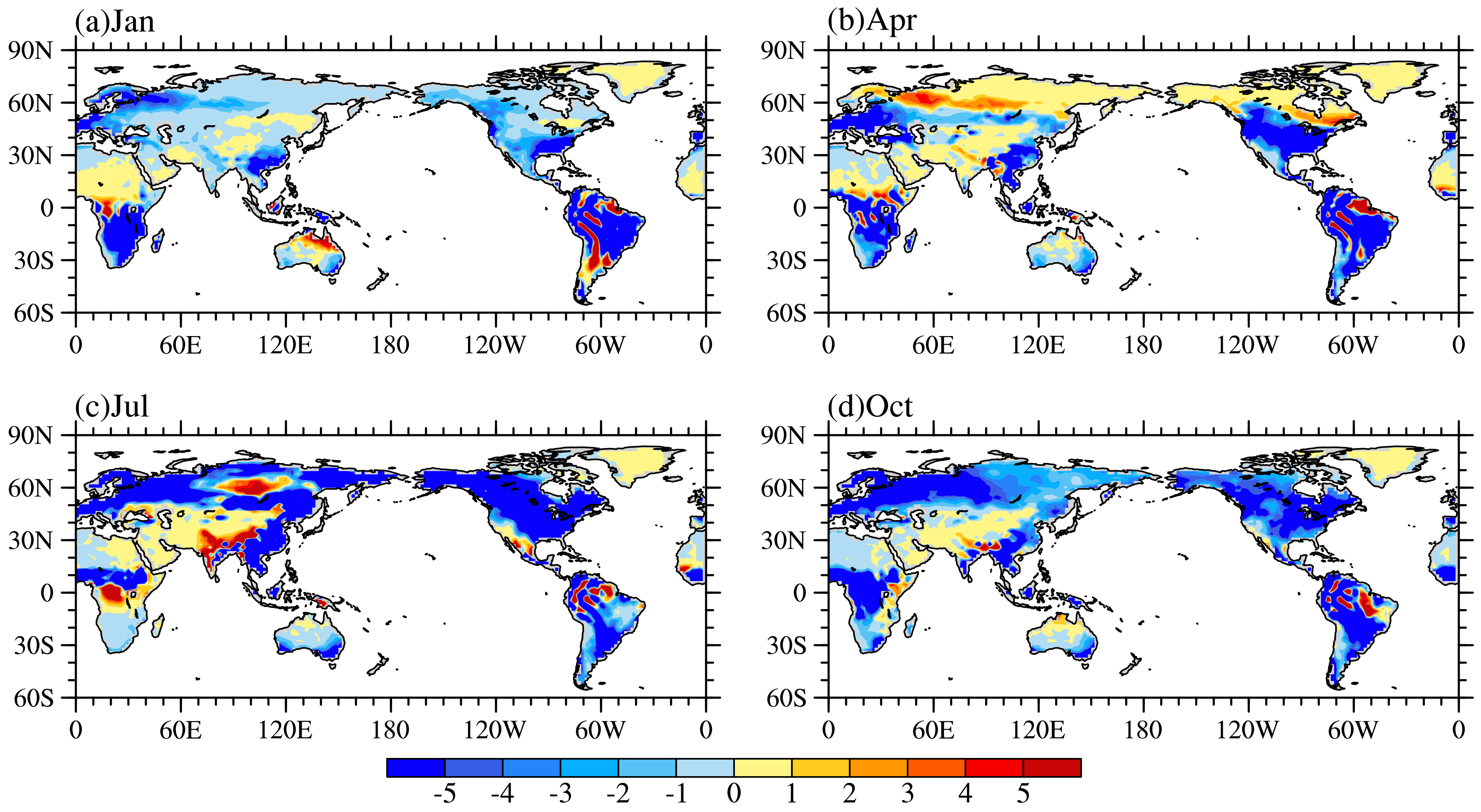
Figure 6.
Spatial distribution of global Et (units: W/m2): (a–d) NOAA reanalysis data and (e–h) simulated by CLM4.5.
Figure 6.
Spatial distribution of global Et (units: W/m2): (a–d) NOAA reanalysis data and (e–h) simulated by CLM4.5.
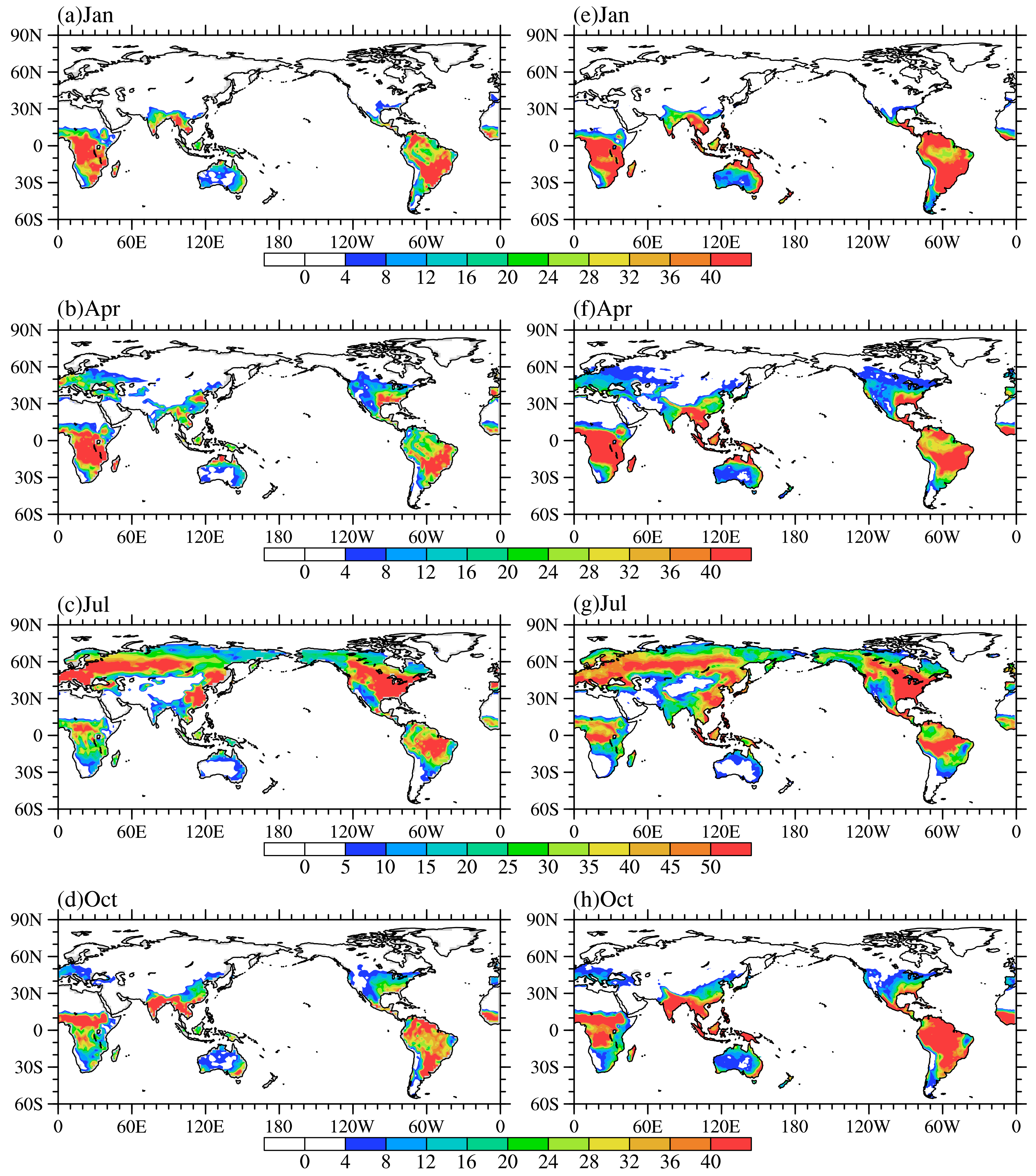
Figure 7.
Spatial distribution of global Et (units: W/m2): (a–d) difference between CLM4.5 and NOAA, (e–h) difference between CLM4.0 and NOAA, and (i–l) difference between CLM4.5 and CLM4.0.
Figure 7.
Spatial distribution of global Et (units: W/m2): (a–d) difference between CLM4.5 and NOAA, (e–h) difference between CLM4.0 and NOAA, and (i–l) difference between CLM4.5 and CLM4.0.

Figure 8.
Spatial distribution of global Es (units: W/m2): (a–d) CFSR reanalysis data and (e–h) simulated by CLM4.5.
Figure 8.
Spatial distribution of global Es (units: W/m2): (a–d) CFSR reanalysis data and (e–h) simulated by CLM4.5.

Figure 9.
Spatial distribution of global Es (units: W/m2): (a–d) difference between CLM4.5 and CFSR, (e–h) difference between CLM4.0 and CFSR, and (i–l) difference between CLM4.5 and CLM4.0.
Figure 9.
Spatial distribution of global Es (units: W/m2): (a–d) difference between CLM4.5 and CFSR, (e–h) difference between CLM4.0 and CFSR, and (i–l) difference between CLM4.5 and CLM4.0.

Figure 10.
Spatial distribution of global latent heat flux (units: W/m2): (a–d) FLUXNET data and (e–h) simulated by CLM4.5.
Figure 10.
Spatial distribution of global latent heat flux (units: W/m2): (a–d) FLUXNET data and (e–h) simulated by CLM4.5.
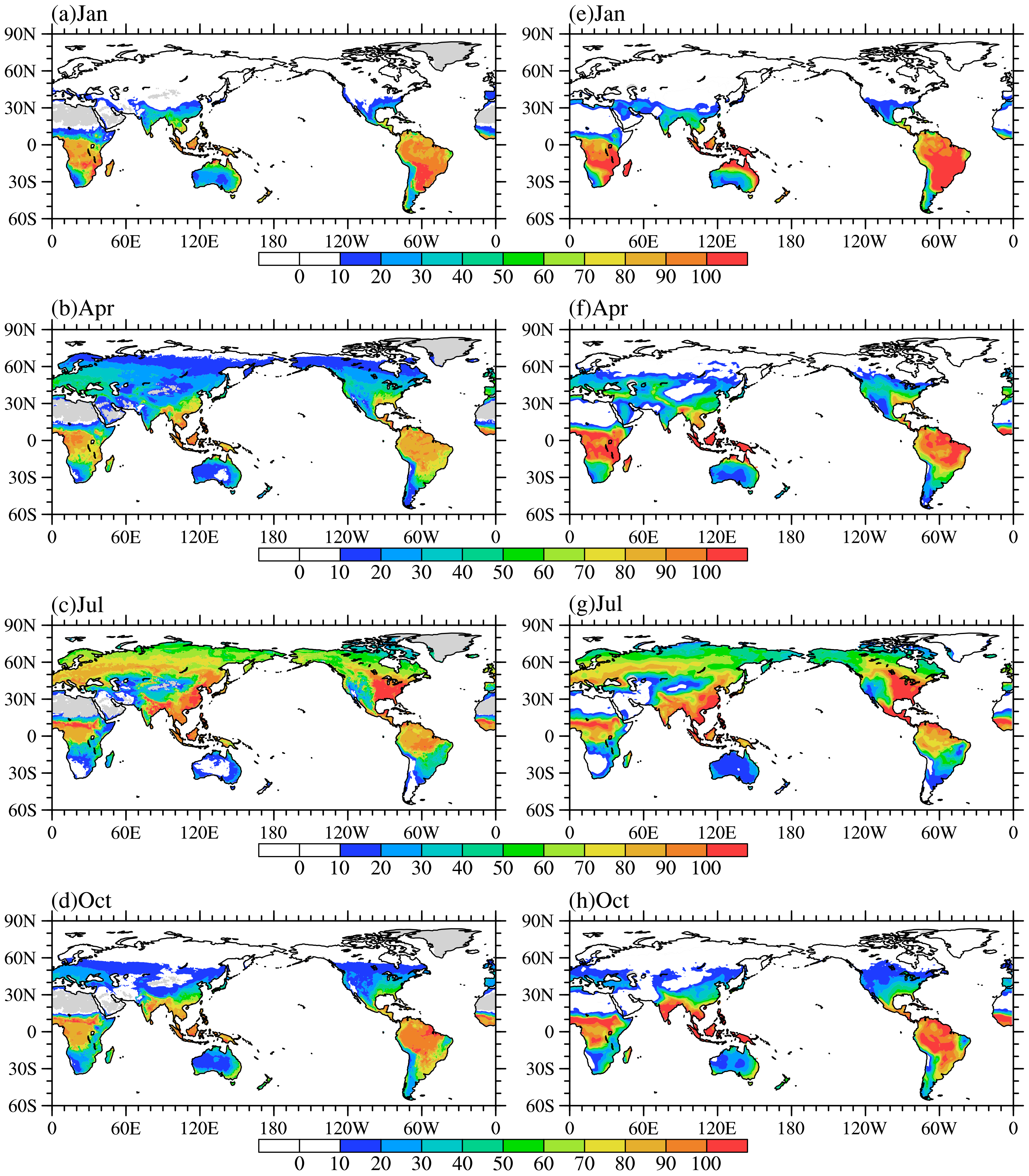
Figure 11.
Spatial distribution of global latent heat flux (units: W/m2): (a–d) difference between CLM4.5 and FLUXNET, (e–h) difference between CLM4.0 and FLUXNET, and (i–l) difference between CLM4.5 and CLM4.0.
Figure 11.
Spatial distribution of global latent heat flux (units: W/m2): (a–d) difference between CLM4.5 and FLUXNET, (e–h) difference between CLM4.0 and FLUXNET, and (i–l) difference between CLM4.5 and CLM4.0.

Table 1.
The root mean square errors (RMSEs), means and spatial correlation coefficients (SCC) for global Ec in January, April, July, and October and annual mean.
Table 1.
The root mean square errors (RMSEs), means and spatial correlation coefficients (SCC) for global Ec in January, April, July, and October and annual mean.
| RMSE (Units: W/m2) | Mean (Units: W/m2) | SCC | ||
|---|---|---|---|---|
| CLM4.5 | NOAA | |||
| January | 7.6 | 3.3 | 5.4 | 0.91 |
| April | 7.1 | 4.3 | 6.6 | 0.91 |
| July | 10.1 | 6.1 | 10.6 | 0.85 |
| October | 7.6 | 3.3 | 6.4 | 0.89 |
| Annual mean | 6.4 | 4.3 | 7.3 | 0.90 |
Table 2.
RMSEs, means and spatial correlation coefficients (SCC) for globally Et in January, April, July and October and annual mean.
Table 2.
RMSEs, means and spatial correlation coefficients (SCC) for globally Et in January, April, July and October and annual mean.
| RMSE (Units: W/m2) | Mean (Units: W/m2) | SCC | |||||
|---|---|---|---|---|---|---|---|
| CLM4 | CLM4.5 | CLM4 | CLM4.5 | NOAA | CLM4 | CLM4.5 | |
| January | 8.7 | 7.3 | 8.2 | 7.5 | 6.2 | 0.88 | 0.89 |
| April | 9.6 | 7.5 | 9.7 | 9.4 | 7.5 | 0.84 | 0.88 |
| July | 12.8 | 11.0 | 17.7 | 18.1 | 17.3 | 0.84 | 0.89 |
| October | 10.5 | 8.0 | 9.3 | 8.9 | 7.1 | 0.84 | 0.89 |
| Annual mean | 8.3 | 6.0 | 11.0 | 10.7 | 9.4 | 0.86 | 0.91 |
Table 3.
Annual mean of the Et (Unit: W/m2) of the dominant PFTs in CLM4.0 and CLM4.5 and their difference (CLM4.5-CLM4.0).
Table 3.
Annual mean of the Et (Unit: W/m2) of the dominant PFTs in CLM4.0 and CLM4.5 and their difference (CLM4.5-CLM4.0).
| PFT Number | PFT Name | CLM4.0 | CLM4.5 | CLM4.5-CLM4.0 |
|---|---|---|---|---|
| 16 | C3 dry land crops | 21.0 | 23.7 | 2.7 |
| 11 | temperate deciduous shrubs | 7.6 | 8.9 | 1.3 |
| 13 | boreal grassland | 6.8 | 7.3 | 0.4 |
| 14 | C3 grassland | 6.1 | 7.4 | 1.4 |
| 15 | C4 grassland | 23.1 | 24.7 | 1.6 |
| 12 | north deciduous broad-leaved shrubs | 10.0 | 12.2 | 2.2 |
| 5 | tropical evergreen broad-leaved forests | 54.9 | 43.4 | −11.5 |
| 3 | northern evergreen coniferous forests | 9.0 | 11.1 | 2.1 |
Table 4.
RMSEs, means and spatial correlation coefficients (SCC) for globally Es in January, April, July and October and annual mean.
Table 4.
RMSEs, means and spatial correlation coefficients (SCC) for globally Es in January, April, July and October and annual mean.
| RMSE (Units: W/m2) | Mean (Units: W/m2) | SCC | |||||
|---|---|---|---|---|---|---|---|
| CLM4 | CLM4.5 | CLM4 | CLM4.5 | NOAA | CLM4 | CLM4.5 | |
| January | 9.1 | 8.5 | 5.4 | 5.2 | 4.5 | 0.61 | 0.64 |
| April | 11.3 | 11.1 | 8.0 | 7.5 | 8.5 | 0.51 | 0.52 |
| July | 12.3 | 11.4 | 11.4 | 10.9 | 10.5 | 0.54 | 0.58 |
| October | 9.7 | 8.6 | 6.4 | 7.0 | 6.9 | 0.49 | 0.53 |
| Annual mean | 8.5 | 7.9 | 7.8 | 7.5 | 7.6 | 0.50 | 0.53 |
Table 5.
RMSE, means and spatial correlation coefficients (SCC) for globally latent heat flux in January, April, July and October and annual mean.
Table 5.
RMSE, means and spatial correlation coefficients (SCC) for globally latent heat flux in January, April, July and October and annual mean.
| RMSE (Units: W/m2) | Mean (Units: W/m2) | SCC | |||||
|---|---|---|---|---|---|---|---|
| CLM4 | CLM4.5 | CLM4 | CLM4.5 | FLUXNET | CLM4 | CLM4.5 | |
| January | 13.2 | 12.1 | 16.7 | 15.8 | 15.4 | 0.97 | 0.97 |
| April | 16.5 | 15.2 | 21.7 | 21.0 | 20.5 | 0.93 | 0.92 |
| July | 15.8 | 14.5 | 34.8 | 34.7 | 30.4 | 0.87 | 0.88 |
| October | 12.3 | 10.2 | 18.9 | 19.0 | 18.1 | 0.97 | 0.96 |
| Annual mean | 9.7 | 11.8 | 22.8 | 22.3 | 20.7 | 0.93 | 0.91 |
Table 6.
The temporal correlation coefficient of the bias between latent heat flux and its components in some problematic regions (* indicates not pass significance test at significance level of 0.05).
Table 6.
The temporal correlation coefficient of the bias between latent heat flux and its components in some problematic regions (* indicates not pass significance test at significance level of 0.05).
| Southeastern China | Siberia | Southeastern United States | Amazon | Europe | |
|---|---|---|---|---|---|
| Ec | −0.29 | 0.10 * | −0.38 | −0.21 | −0.31 |
| Et | −0.32 | −0.34 | −0.23 | 0.46 | −0.05 * |
| Es | 0.46 | 0.70 | 0.61 | −0.03 * | 0.74 |
© 2018 by the authors. Licensee MDPI, Basel, Switzerland. This article is an open access article distributed under the terms and conditions of the Creative Commons Attribution (CC BY) license (http://creativecommons.org/licenses/by/4.0/).
Share and Cite
MDPI and ACS Style
Yang, M.; Zuo, R.; Wang, L.; Chen, X. A Simulation Study of Global Evapotranspiration Components Using the Community Land Model. Atmosphere 2018, 9, 178. https://doi.org/10.3390/atmos9050178
AMA Style
Yang M, Zuo R, Wang L, Chen X. A Simulation Study of Global Evapotranspiration Components Using the Community Land Model. Atmosphere. 2018; 9(5):178. https://doi.org/10.3390/atmos9050178
Chicago/Turabian StyleYang, Minghao, Ruiting Zuo, Liqiong Wang, and Xiong Chen. 2018. "A Simulation Study of Global Evapotranspiration Components Using the Community Land Model" Atmosphere 9, no. 5: 178. https://doi.org/10.3390/atmos9050178
Note that from the first issue of 2016, this journal uses article numbers instead of page numbers. See further details here.