Using Shortwave Radiation to Evaluate the HARMONIE-AROME Weather Model

1
Danmarks Meteorologiske Institut, DK-2100 Copenhagen, Denmark
2
Met Éireann, 65/67 Glasnevin, Dublin 9, D09 Y921, Ireland
*
Author to whom correspondence should be addressed.
†
These authors contributed equally to this work.
Atmosphere 2018, 9(5), 163; https://doi.org/10.3390/atmos9050163
Submission received: 5 March 2018
/
Revised: 10 April 2018
/
Accepted: 12 April 2018
/
Published: 26 April 2018
(This article belongs to the Special Issue Energy Meteorology)
Abstract
:Evaluation of global shortwave irradiance forecasts from the HARMONIE-AROME weather prediction model is presented in this paper. We give examples of how such an evaluation can be used when testing a weather model or reanalysis product. We specifically use the non-dimensional clear sky and variability indices. We have tested seven months of HARMONIE-AROME 40h1.1 output against Danish global irradiance stations and 35 years of the Irish Met Éireann reanalysis (MÉRA) simulations. MÉRA, which is run with HARMONIE-AROME 38h1.2, is shown to have a significantly lower bias than the previously available global horizontal irradiance (GHI) reanalysis data from the ERA-Interim dataset. The Danish HARMONIE-AROME 40h1.1 has a negative bias during the summer months that is not seen in the Irish HARMONIE-AROME 38h1.2. For both model runs, we find a negative bias in the shortwave irradiance forecasts on days with thick clouds. This suggest that the model has too much cloud water in thick clouds.
Keywords:
solar irradiance; clear sky index; variability index; Ireland; Denmark; HARMONIE-AROME; MÉRA1. Introduction
Forecasting clouds poses the biggest challenge in everyday weather model operations. This is a problem particularly for aviation and solar energy purposes. Reanalysis datasets have also been tested and found to be lacking in quality compared to satellite-derived cloud datasets [1]. Clearly, cloud forecasting needs to be improved. However, this is not easy because clouds are affected by several atmospheric processes, the model surface physics and assumed climatologies.
In order to improve cloud forecasts and reanalyses, it is necessary to perform a detailed quantitative evaluation. Cloud cover is often used to evaluate cloud forecasts. However, this is not a good metric due to inconsistent methods for assessing the cloud cover. Some ceilometers only measure clouds up to a height of 7 km (e.g., [2]), and thus, cirrus clouds are not included as part of the cloud cover. In some countries, the cloud cover is assessed by a human observer who can see the full sky unlike a ceilometer, which normally measures only at zenith. Tests have shown that this can cause markedly different cloud cover evaluation results across country boundaries [3].
Global horizontal irradiance (GHI), also referred to as “global radiation”, provides an objective and quantitative measure for evaluating cloud forecasts during the daytime. GHI is the shortwave irradiance integrated over all downward directions and wavelengths in the solar spectrum received by a horizontal surface of unit area. Furthermore, non-dimensional indices for solar energy resource assessment have been developed in recent years and decades that are very useful. One such index is the clear sky index (CSI), which is the GHI divided by the theoretical GHI during clear sky conditions, e.g., [4,5]. In this paper, we use the theoretical GHI clear sky model of [6,7], which includes coefficients that account for variable integrated atmospheric water vapour, aerosols and ozone. Another non-dimensional index that we will use here is the daily variability index (VI) as introduced by [8]. This VI is essentially the relative length of the daily curve of actual measured GHI to the daily curve of GHI under clear sky conditions. In this manner the relative variability of morning and evening periods with low GHI are not weighted disproportionally to the periods with high GHI during the middle of the day. In our analyses, we use the daily VI and a daily averaged GHI weighted CSI to make bins in which we can test the HARMONIE-AROME weather model GHI forecast under specific cloud conditions. Our hypothesis is that such a binned GHI evaluation will help in identifying weaknesses in the model.
2. Datasets/Models
2.1. Observation Networks
2.1.1. The Irish Network
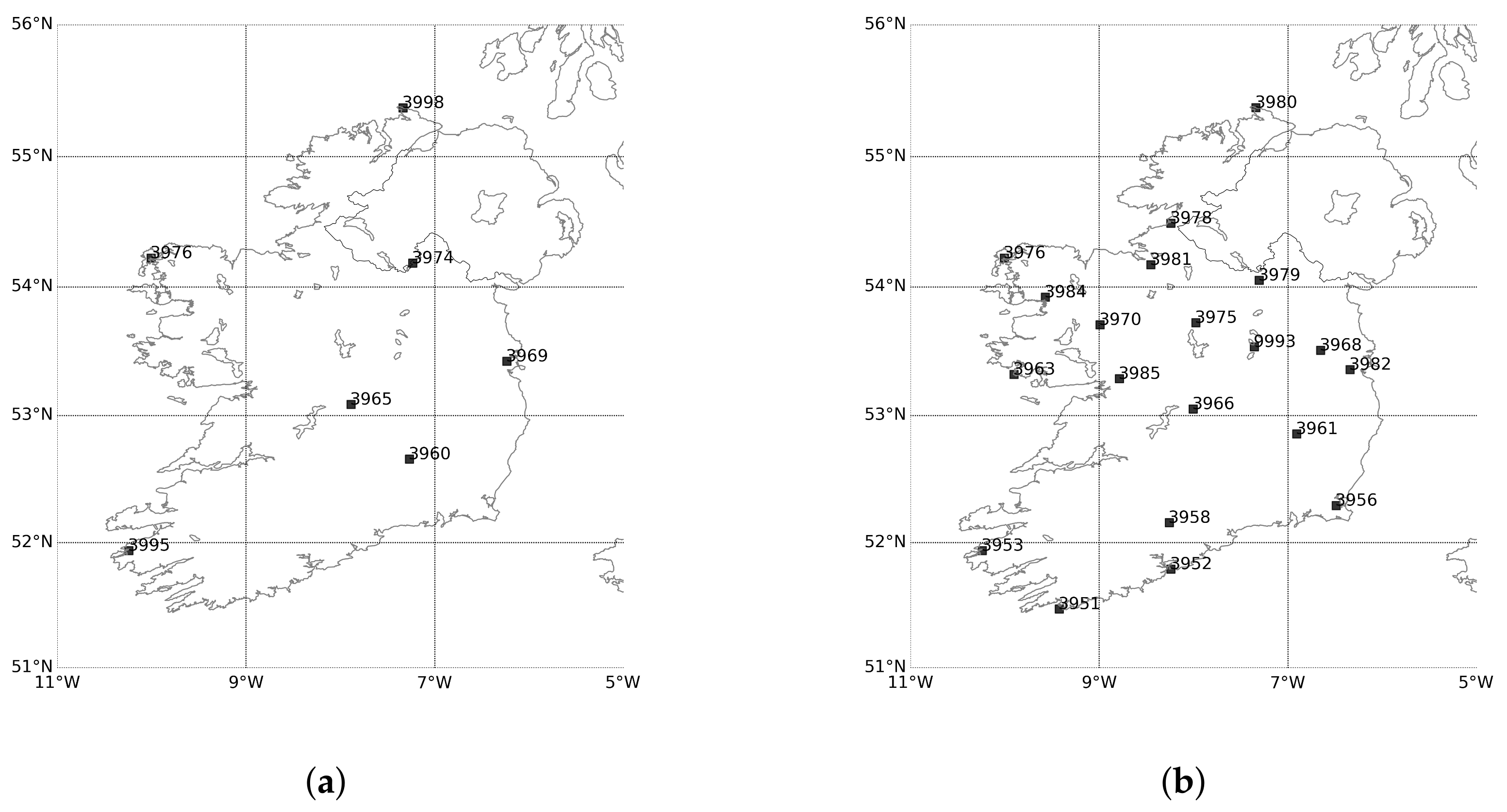
A GHI network was established in Ireland in 1954 when the first pyranometers were installed by the Irish Meteorological Service, Met Éireann, at Valentia Observatory in the southwest of the country. Over the next few decades, a further six stations were added to the network, the locations of which are shown in Figure 1a [9]. From 2008 onwards, the network underwent a process of automation with some of the original stations moving to more appropriate nearby sites. This automated network (referred to as the TUCSON network) is shown in Figure 1b. The stations are equipped with Kipp and Zonen CMP11 pyranometers (2628 XH Delft, Netherlands) which are “Secondary Standard pyranometers”, but are more accurate than “First Class Pyranometers”.
2.1.2. The Danish Network
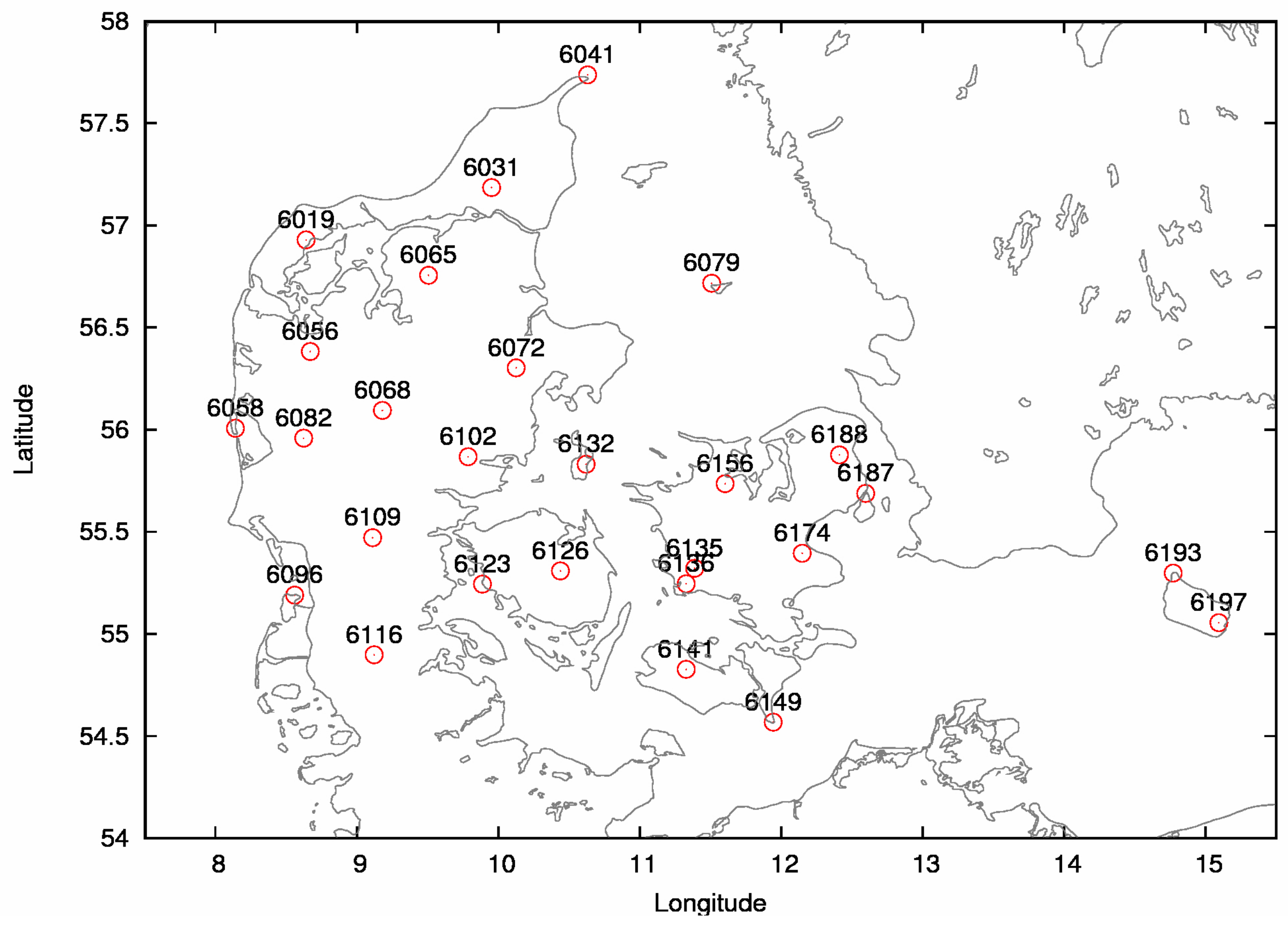
Since the beginning of 2001, the Danish Meteorological Institute, DMI, has measured GHI at 13 stations across Denmark. In the years up to 2011, this network was expanded to include 28 stations that are all still operational. The distribution of these stations across the country can be seen in Figure 2. Before 2001, the sunshine duration has been monitored since 1920 [10]. The GHI stations are all equipped with Star 8101 pyranometers (Schenk GmbH, A-1210 Wien, Austria), which are “First Class Pyranometers” according to the ISO 9060 standard.
2.2. Models
2.2.1. MÉRA
Met Éireann has carried out a 35-year very high resolution (2.5-km horizontal grid) regional climate reanalysis for Ireland using the ALADIN-HIRLAM numerical weather prediction system and in particular the HARMONIE-AROME canonical configuration of this system (see [11] for details on the model, acronym definitions and an overview of the reanalysis). This Met Éireann reanalysis, abbreviated MÉRA, spans the years 1981 to 2015. An analysis of surface parameters including screen-level and soil temperatures, 10-m wind speeds, mean sea-level pressure and precipitation is presented in [11,12]. This paper extends the analysis of MÉRA to include an evaluation of GHI with particular emphasis on its use in the validation of clouds.
Version 38h1.2 of the ALADIN-HIRLAM system was used to carry out the MÉRA simulations. This canonical configuration of HARMONIE-AROME was run on a horizontal grid of 2.5-km spacing, using 65 vertical levels and a model top of 10 hPa. The data assimilation component of the model is described in [13,14]; the forecast component is described in [15] with more recent updates included in [16]. The SURFEX externalized surface scheme Version 7.2 [17] is used for surface data assimilation and the modelling of surface processes. A summary of the model details is presented in Table 1.
Conventional observations (i.e., from synoptic stations (SYNOP), ships, drifting buoys (DRIBU), radiosonde ascents (TEMP) and aircraft (AIREP, AMDAR) were assimilated. These observations are the same as those used by the European Centre for Medium Range Weather Forecasts’ (ECMWF) ERA-Interim reanalysis [18]. Locally available SYNOP observations were used to fill gaps in the ERA-Interim SYNOP observation archive to ensure cycle continuity and successful data assimilation each cycle. MÉRA uses a three-hour forecast cycle with surface and upper-air data assimilation. Three-hour forecasts were produced for each cycle except the midnight (00 UTC) cycle when a 33-h forecast was produced.
2.2.2. Danish Model Runs
Operational weather model runs from DMI are included for the seven-month period from June to December 2017. Specifically, output from the HARMONIE-AROME 40h1.1 model run covering the Northern Europe A (NEA) domain of DMI is included. The physics in this model version has been described in detail by [16] with the specific NEA setup described by [19]. In Table 2, an overview of the NEA setup is given. As can be seen, this setup has the same horizontal and vertical resolution as MÉRA, but includes significantly more observations for data assimilation. In particular, the DMI setup includes additional aircraft data (MODE-S, EHS), satellite data (AMSU-A, MHS, ATMS, MSG, Metop-A, Metop-B, COSMIC) and radar data from the European OPERA radar network.
HARMONIE-AROME 40h1.1 is the model version release that followed immediately after HARMONIE-AROME 38h1.2 used for MÉRA. The differences between the model versions as run operationally at DMI (NEA; 40h1.1) and run for the long-term reanalysis at Met Éireann (MÉRA; 38h1.2) are too extensive to list here. The following major changes, which affect the cloud cover and cloud transmittance, we would, however, like to mention. Firstly, the externalized surface scheme has been updated to Version 7.3 [20]. Secondly, the so-called cloud-inhomogeneity factor has been changed from 0.7 to 1.0 as suggested by [21], which means that the cloud optical thickness is no longer reduced by 30% before the cloud transmittance is computed. Thirdly, the Cuxart, Bougeault and Redelsperger (CBR) turbulence scheme [22] has been replaced by the turbulence scheme from the RACMO model [23].
Note that all of the results for Irish stations are compared to all of the MÉRA reanalysis dataset, which spans the years 1981 to 2015. The MÉRA domain does not include Denmark. Hence, the Danish analysis has been carried out using using HARMONIE-AROME operational NWP simulations for May to December 2017.
3. Results
3.1. GHI Statistics
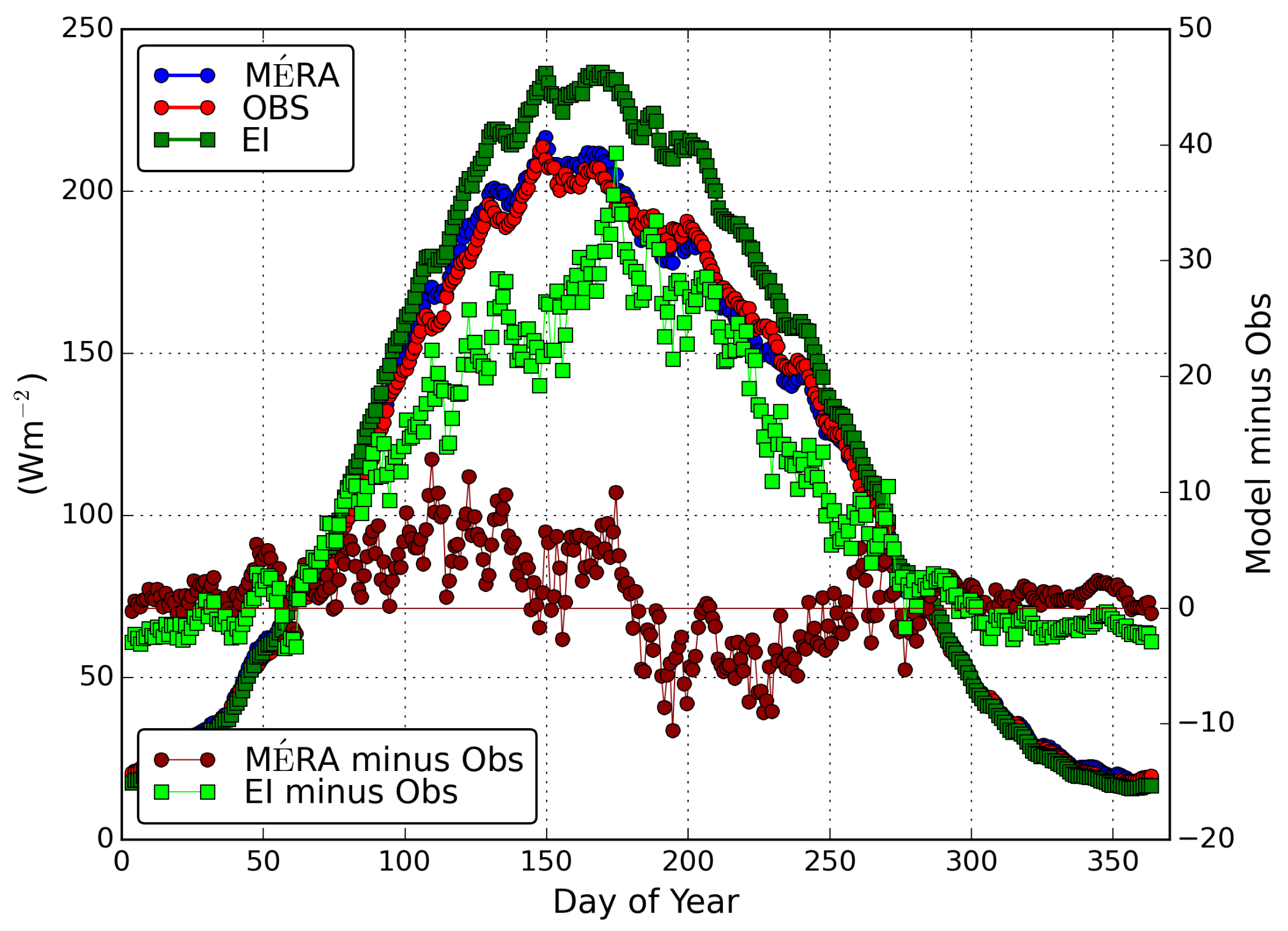
The seven original stations in the Irish network were used to create Figure 3, which shows the daily mean GHI as a function of the day of the year for observations and the MÉRA dataset. 24-h GHI MÉRA forecasts for the years 1981 to 2015 are included. These forecasts were initiated at 00 UTC. Output from the ERA-Interim reanalysis is also included as a comparison and highlights the benefits of the high resolution MÉRA dataset over the coarse resolution ERA-Interim (79 km grid spacing approximately). Twenty four-hour forecasts of accumulated GHI were extracted from the MÉRA and ERA-Interim datasets, interpolated to each Irish station using bilinear interpolation and averaged over the full day. The biases in ERA-Interim are small and mostly negative in winter (a few Wm−2), but are otherwise positive and up to 40 Wm−2 in summer. On the other hand, the biases in MÉRA are smaller (±10 Wm−2) (positive except for a period in July and August, where the bias is slightly negative overall). Because the MÉRA dataset is clearly more suitable than ERA-Interim as regards GHI because of its higher resolution, the remainder of the reanalysis comparisons are restricted to the MÉRA dataset. In addition, hourly outputs of GHI are available from MÉRA, whereas only daily accumulations of GHI are available from ERA-Interim.
In Figure 4, the observed and modelled time series of the average of all Danish GHI stations are shown. The averages are hourly averages over the full day. As only seven months of data were available, these results are less clear than the MÉRA results, but an average negative bias of −10 to −20 Wm−2 can be seen in the period from June to September, while the last three months have little bias.
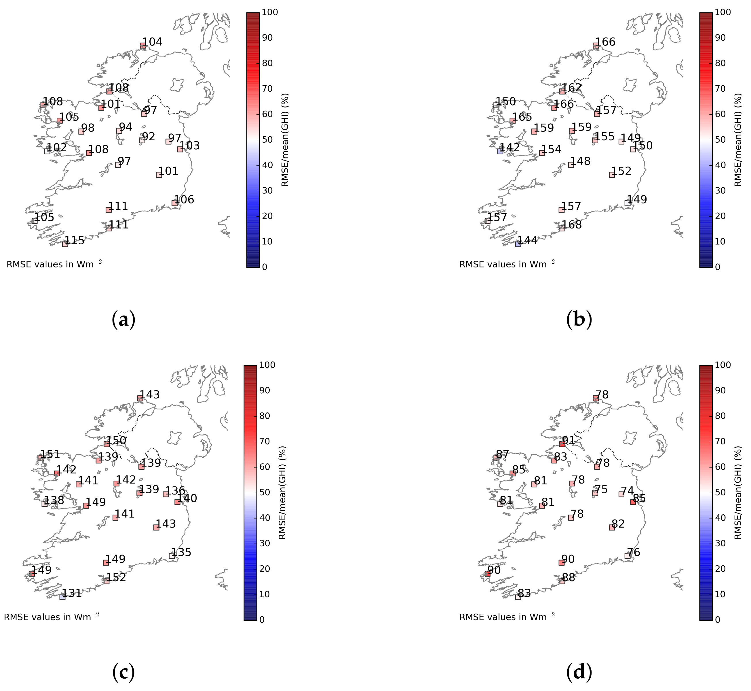
To analyse the biases in MÉRA relative to observations in more detail, the mean daily biases in GHI by month averaged over all available years (2008 to 2014) were calculated for the TUCSON network of 20 stations. The biases in MÉRA relative to observations are positive between February and June and in September, the exceptions being some of the western stations. In July, the biases are positive in the east, but negative in the west. In August, the biases are negative except for a few eastern stations. From October to January, the biases are mostly negative with some exceptions for stations near the coasts (see Figure 5 for biases for a selection of months). RMSE (root mean square error) plots are also included for completeness in Figure 6.
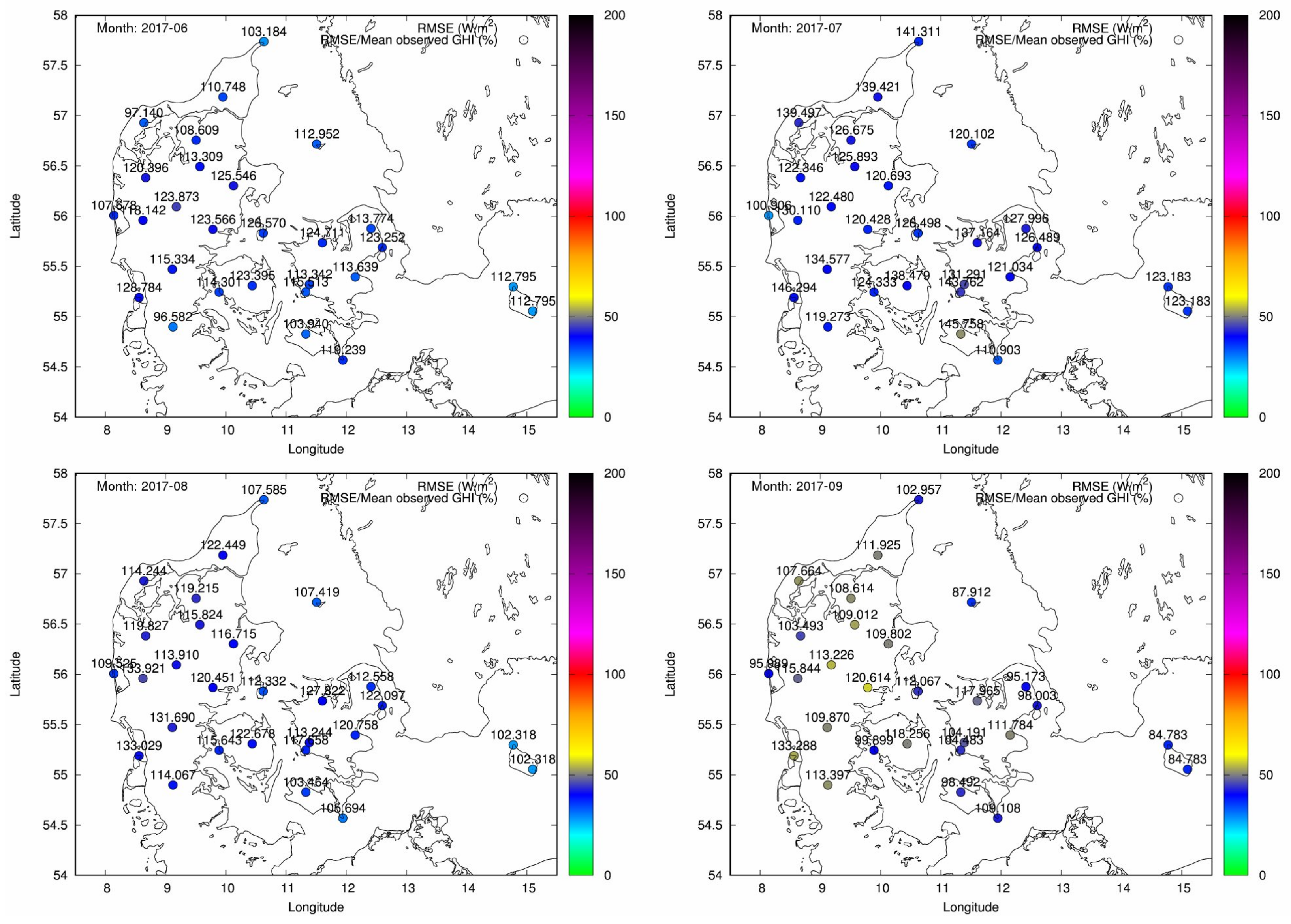
Likewise for the Danish stations, monthly statistics for four selected months (June, July, August, September) are shown in Figure 7, Figure 8 and Figure 9. This includes maps of bias (Figure 7) and RMSE (Figure 8) for each station and a plot of the same data shown graphically in order to make the variations easier to quantify. From the Danish model runs, hourly GHI forecasts up to 12 hours ahead initiated at 00 and 12 UTC are used in these statistics.
3.2. Clear Sky Index
The definition of clear sky index (CSI) used here involves the ratio of GHI divided by the theoretical GHI during clear sky conditions, e.g., [4,5], which is dependent on the location, date and time. In particular, we used the theoretical GHI clear sky model of [6,7], which includes coefficients that account for variable integrated atmospheric water vapour and, if available, aerosols and ozone. In the Danish weather model runs, the integrated water vapour variations were available and have been accounted for. In the comparisons involving MÉRA, we assumed an atmosphere with an integrated water vapour load of 2.5 g·cm−2, which is a typical load for a mid-latitude location like Ireland. Variable atmospheric water vapour was of course included in the MÉRA run, but these data are not readily available.
Figure 10 shows a time series of weighted daily CSI for MÉRA, calculated using hourly CSI weighted by hourly GHI and summed over the day for hours when the sun was above the horizon. Note that GHI for each hour was calculated using the accumulated GHI for consecutive hours extracted from the 0 to 33 h forecasts run at 00 Z . CSI was also averaged over all stations, and a 30-day running mean was applied to aid visualisation. CSI trends based on observations and on MÉRA are shown in the figure, as well as the bias in MÉRA relative to observations. On average, there is very good agreement between MÉRA and observations, but monthly mean biases in daily weighted CSI of ±0.2 can be seen. Figure 11 shows a frequency distribution of weighted daily CSI for the TUCSON stations. Overall, there is good agreement, but a small shift towards higher CSIs in MÉRA for most of the stations. MÉRA has significantly more cases for the lowest CSI bin, i.e., for clear sky indices from 0.0 to 0.1, than the observations.
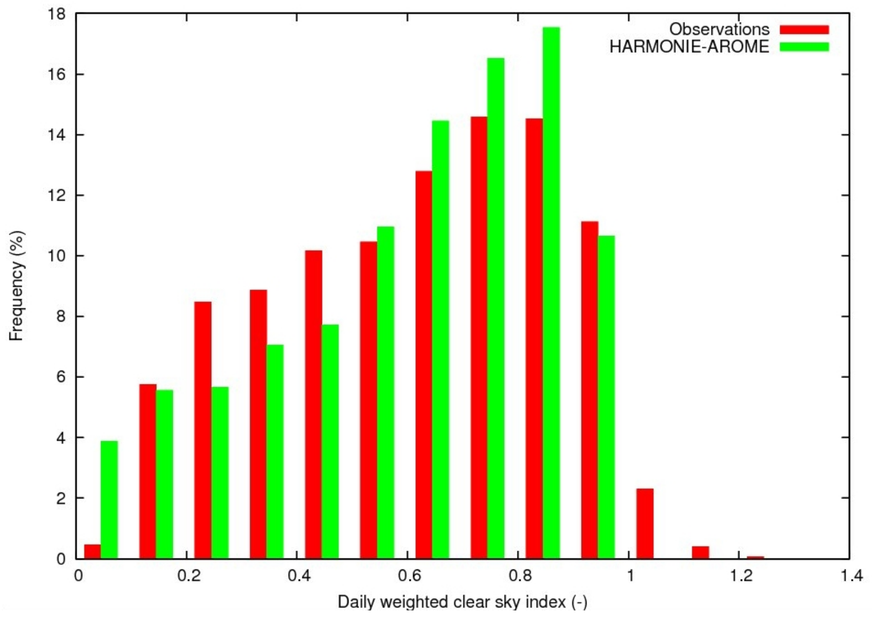
Similarly, the frequency distribution of the Danish daily weighted CSIs are shown in Figure 12. In this case, the modelled CSIs never exceed 1.0, but the observed CSIs do so in approximately 3% of the cases. In the lower part of the frequency distribution, it can be seen that the NEA HARMONIE-AROME runs have significantly more cases in the lowest CSI bin, i.e., for clear sky indices from 0.0 to 0.1, than the observations, as was also seen for the MÉRA data (Figure 11).
3.3. Variability Index
The daily variability index (VI) of [8] is essentially the relative length of the daily curve of actual measured GHI to the daily curve of GHI in clear sky conditions. See Equation (1) below, where CSGHI is the GHI under clear sky conditions, k is the time index (here, hour of the day) and t is 60 min in this case, as we only have hourly GHI available from the model runs. Using this definition, the relative variability of morning and evening periods with low GHI are not weighted disproportionately to the periods with high GHI during midday. The advantage of using the VI is that a high VI indicates situations with subgrid-scale variability that is unresolved in the weather model runs. It is interesting to test whether the models have errors due to sub-grid cloud variability. In general, the VI provides a method to classify cloud situations.
Figure 13 shows a time series of daily VI averaged over all TUCSON stations with a 30-day running mean applied to aid visualisation. VI trends based on observations and on MÉRA are shown in the figure, as well as the bias in MÉRA relative to observations. On average, there is very good agreement between MÉRA and observations with monthly mean biases in the range ±2. A pronounced seasonal cycle in VI is also evident over the seven-year period with the greatest variability during spring/summer when convective events are more common in Ireland compared to lower variability in autumn/winter, where overcast days with low stratus cloud are more typical. Similar results were found for the HARMONIE-AROME NEA run (not shown here).
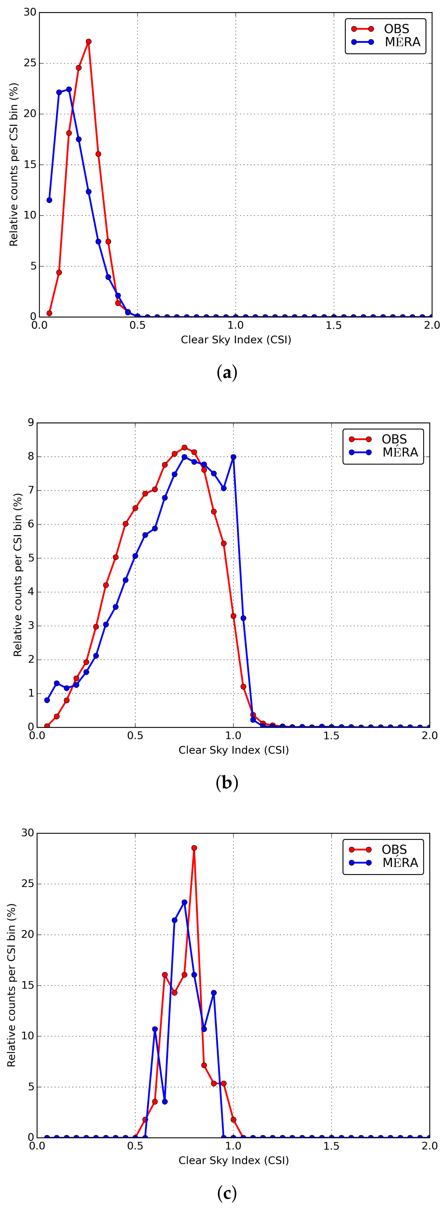
The final part of this analysis merges both the CSI and VI with the aim of testing the GHI forecasts from the HARMONIE-AROME weather model under specific cloud conditions in order to identify weaknesses in the model. Figure 13 shows that the VI for Ireland mostly ranges between five and 10. Figure 14 shows very good agreement between MÉRA and observations for weighted daily CSI for VI values in the range of 10 to 15 (i.e., the most variable days cloud-wise). Here, we have plotted the weighted daily CSI for three VI bin ranges (0 to 5, 5 to 10 and 10 to 15). The middle VI range (5 to 10) shows good agreement overall with a small shift towards higher CSIs in MÉRA. The lowest VI range (0 to 5) shows a negative bias, which is consistent with the results for the lowest CSI bin in Figure 11.
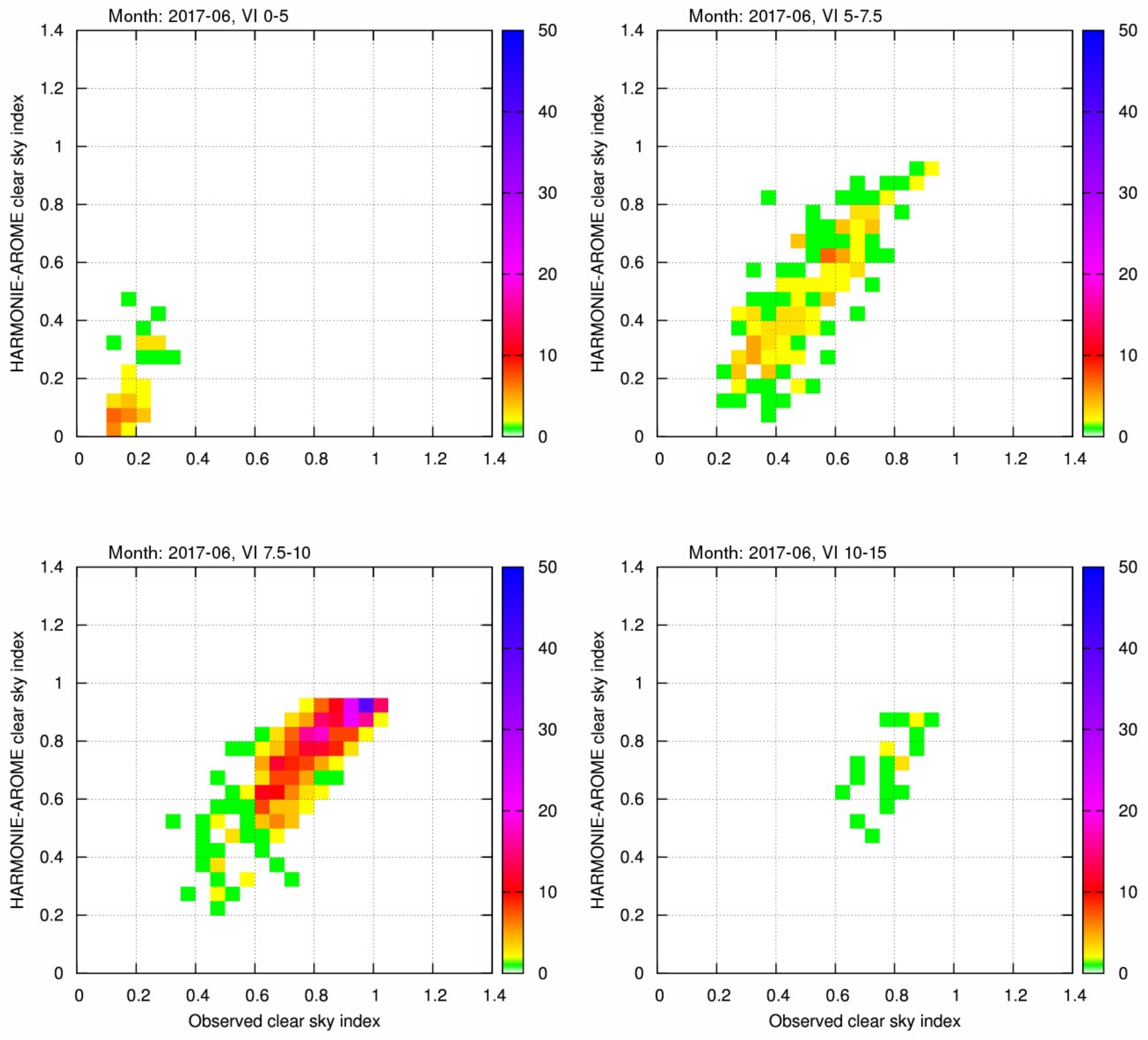
Another way of visualising the CSI and VI results is shown in Figure 15. Here, binned 2D histograms of the modelled and observed CSI values are shown for the HARMONIE-AROME NEA model compared with the Danish GHI stations. These are similar to contingency tables used for precipitation evaluation and are made for four VI bins: 0 to 5, 5 to 7.5, 7.5 to 10 and 10 to 15. Ideally, all the data should follow the diagonal at which the model CSI values are equal to the observed CSI values. Here, negative deviations in the model data are seen for the lowest CSI and VI values in the upper left panel. This is consistent with the frequency distribution seen for the lowest CSI bin in Figure 12. Another negative deviation is seen for the highest CSI values in the bin that contains most of the cases in the lower left panel of Figure 15.
4. Discussion
The high resolution MÉRA dataset captures the variation in global SW irradiance much better than the coarser resolution ERA-Interim dataset. The bias in ERA-Interim relative to observations is mostly positive and up to 30 Wm−2 in summer. On the other hand, MÉRA has much lower biases on average (mostly within 10 Wm−2 and positively biased during the first half of the year, but negatively biased during the last half of the summer months). A similar analysis was carried out using data from the Irish TUCSON network of 20 stations available from 2008 onwards where the data are archived at one-minute resolution. This dataset yielded similar results (not included) to those shown in Figure 3. The MÉRA dataset is thus better suited for solar resource assessment than ERA-Interim for the region covered, i.e., Ireland and the United Kingdom.
Analyses of both datasets as a function of the day of the year and month by month show the variations of the model bias during the course of the year. This could be related to the monthly climatological fields that are used in the model. Several of these are needed to simulate the surface variability such as the evapotranspiration of the assumed vegetation. In countries with a large crop fraction, the vegetation varies greatly, in particular as a result of harvest. This also affects the cloud cover and, in turn, the GHI. Monthly aerosol climatologies [24,25] are also assumed in HARMONIE-AROME, which affect the GHI [26,27].
In Figure 14 and Figure 15, there is a shift towards lower CSI for MÉRA compared to observations for the low VI range (0 to 5), which is consistent with cloud water loads that are too high. Tests against satellite-derived cloud water loads also show this [7]. This bias does not count much for the overall GHI statistics, but it could be important for the cloud microphysical processes in the model that initiate precipitation.
Although the differences between the results shown here for the NWP model output for Ireland and Denmark could be due to geographical differences, we find it likely that changes in the HARMONIE-AROME model from Version 38h1.2 to Version 40h1.1 are important. In particular, the change of the cloud inhomogeneity factor from 0.7 to 1.0, as discussed by [21], reduces the cloud transmittance. This means that the cloud transmittance is lower in Version 40h1.1 as run for HARMONIE-AROME NEA than in Version 38h1.2 used for MÉRA. In theory, cloud inhomogeneity effects are largest when the clouds are most variable. This fits with the negative bias seen in Figure 9 and in the lower left panel of Figure 15, which is not seen in the right-hand panel of Figure 14. We suggest a cloud inhomogeneity factor that is reduced when variable clouds are present to be tested using the next model version. Another possible explanation for this is too high aerosol optical depth assumed in the model climatologies over Denmark. This possibility should also be tested.
In order to quality-assure GHI measurements, the ideal radiation station includes a three-component measurement setup, where the direct, diffuse and global irradiance are measured simultaneously. Since the pyranometer calibration can drift over time, such a redundancy of irradiance measurements is recommended [28]. We do not have country-wide measurements of this type, which would have enabled us to draw more firm conclusions from these analyses.
When computing the CSI values for the Danish NEA data, we accounted for the variations in the integrated water vapour. This made the CSI value range more homogeneous across the year and is recommended for computing clear sky irradiance and CSI values. In Figure 11, the CSI frequency distribution plot of the MÉRA data displays CSI values greater than 1.0. These occur during winter, when the atmosphere is very dry and the modelled CSI therefore becomes too high. In Figure 12, CSI values larger than 1.0 do not occur for the HARMONIE-AROME NEA data, but they still occur for the observations. This could be due to too high aerosol absorption and scattering in the assumed clear sky model [6,7].
5. Conclusions
The analyses presented here demonstrate new aspects of how to evaluate and improve numerical weather models. These should be made a standard part of the overall weather model evaluation analyses. In particular, ground-based GHI stations such as those used here give information about the complex cloud overlap and 3D cloud effects that occur at the sub-grid scale level in modelled and satellite-derived data.
Specifically, we have shown the average GHI bias for individual days of the year for the Met Éireann reanalysis (MÉRA) with HARMONIE-AROME 38h1.2 to be within ±10 Wm2 and to be significantly less than the corresponding bias of the ERA-Interim dataset. We have also shown that HARMONIE-AROME 40h1.1 operational runs for Denmark have a larger negative GHI bias during summer than the HARMONIE-AROME 38h1.2 runs for Ireland. In both cases, we find that on days with very low GHI, HARMONIE-AROME has too low GHI. This indicates that too much cloud water is present in the model in cases with thick stratiform clouds.
We suggest that the GHI evaluation be performed as a standard for HARMONIE-AROME and weather models in general and the model cloud physics be adjusted to improve the issues that we have demonstrated.
Author Contributions
K.P.N. suggested the approach used in this work and carried out the analysis using the Danish observations and HARMONIE-AROME simulations for the Danish NEA domain. E.G. compared the high resolution MÉRA reanalysis dataset and the ERA-Interim reanalysis to observations over Ireland. Both authors wrote the paper.
Acknowledgments
The authors would like to thanks Eoin Whelan and John Hanley of the MÉRA project and the ALADIN-HIRLAM consortium who maintain the HARMONIE-AROME code.
Conflicts of Interest
The authors declare no conflict of interest.
References
- Boilley, A.; Wald, L. Comparison between meteorological re-analyses from ERA-Interim and MERRA and measurements of daily solar irradiation at surface. Renew. Energy 2015, 75, 135–143. [Google Scholar] [CrossRef] [Green Version]
- Martucci, G.; Milroy, C.; O’Dowd, C.D. Detection of Cloud-Base Height Using Jenoptik CHM15K and Vaisala CL31 Ceilometers. J. Atmos. Ocean. Technol. 2010, 27, 305–318. [Google Scholar] [CrossRef]
- De Rooy, W. Royal Netherlands Meteorological Institute (KNMI), De Bilt, Netherlands. Personal communication, 2015. [Google Scholar]
- Perez, R.; Ineichen, P.; Seals, R.; Zelenka, A. Making full use of the clearness index for parameterizing hourly insolation conditions. Sol. Energy 1990, 45, 111–114. [Google Scholar] [CrossRef]
- Skartveit, A.; Olseth, J.A.; Tuft, M.E. An hourly diffuse fraction model with correction for variability and surface albedo. Sol. Energy 1998, 63, 173–183. [Google Scholar] [CrossRef]
- Savijärvi, H. Fast radiation parameterization schemes for mesoscale and short-range forecast models. J. Appl. Meteorol. 1990, 437–447. [Google Scholar] [CrossRef]
- Gleeson, E.; Nielsen, K.P.; Toll, V.; Rontu, L.; Whelan, E. Shortwave Radiation Experiments in HARMONIE. Tests of the cloud inhomogeneity factor and a new cloud liquid optical property scheme compared to observations. ALADIN-HIRLAM Newsl. 2015, 5, 92–106. [Google Scholar]
- Stein, J.; Hansen, C.; Reno, M. The Variability Index: A New and Novel Metric for Quantifying Irradiance and PV Output Variability. In Proceedings of the WREF Conference, Denver, CO, USA, 13–17 May 2012. [Google Scholar]
- Irish Meteorological Service. Solar Radiation Observations 1982; Irish Meteorological Service: Dublin, Ireland, 1983.
- Laursen, E.V.; Rosenørn, S. Landstal af Solskinstimer for Danmark; 1920–2002; Tech. Report, 03-19; Danish Meteorological Institute: Copenhagen, Denmark, 2003.
- Gleeson, E.; Whelan, E.; Hanley, J. Met Éireann high resolution reanalysis for Ireland. Adv. Sci. Res. 2017, 14, 49–61. [Google Scholar] [CrossRef]
- Whelan, E.; Gleeson, E.; Hanley, J. An evaluation of MÉRA, a high resolution mesoscale regional reanalysis. JAMC submitted. 2018. [Google Scholar]
- Fischer, C.; Montmerle, T.; Berre, L.; Auger, L.; Ştefănescu, S.E. An overview of the variational assimilation in the ALADIN/France numerical weather-prediction system. Q. J. R. Meteorol. Soc. 2005, 613, 3477–3492. [Google Scholar] [CrossRef]
- Brousseau, P.; Berre, L.; Bouttier, F.; Desroziers, G. Background-error covariances for a convective-scale data-assimilation system: AROME-France 3DVar. Q. J. R. Meteorol. Soc. 2011, 137, 409–422. [Google Scholar] [CrossRef]
- Seity, Y.; Brousseau, P.; Malardel, S.; Hello, G.; Bénard, P.; Bouttier, F.; Lac, C.; Masson, V. The AROME-France Convective-Scale Operational Model. Mon. Weather Rev. 2011, 139, 976–991. [Google Scholar] [CrossRef]
- Bengtsson, L.; Andrae, U.; Aspelien, T.; Batrak, Y.; Calvo, J.; de Rooy, W.; Gleeson, E.; Sass, B.H.; Homleid, M.; Hortal, M.; et al. The HARMONIE–AROME Model Configuration in the ALADIN–HIRLAM NWP System. Mon. Weather Rev. 2017, 145, 1919–1935. [Google Scholar] [CrossRef]
- Masson, V.; Le Moigne, P.; Martin, E.; Faroux, S.; Alias, A.; Alkama, R.; Belamari, S.; Barbu, A.; Boone, A.; Bouyssel, F.; et al. The SURFEXv7. 2 land and ocean surface platform for coupled or offline simulation of earth surface variables and fluxes. Geosci. Model Dev. 2013, 6, 929–960. [Google Scholar] [CrossRef] [Green Version]
- Dee, D.P.; Uppala, S.M.; Simmons, A.J.; Berrisford, P.; Poli, P.; Kobayashi, S.; Andrae, U.; Balmaseda, M.A.; Balsamo, G.; Bauer, P.; et al. The ERA-Interim reanalysis: Configuration and performance of the data assimilation system. Q. J. R. Meteorol. Soc. 2011, 137, 553–597. [Google Scholar] [CrossRef]
- Yang, X.; Andersen, B.S.; Dahlbom, M.; Sass, B.H.; Zhuang, S.; Amstrup, B.; Petersen, C.; Nielsen, K.P.; Nielsen, N.W.; Mahura, A. NEA, the Operational Implementation of HARMONIE 40h1.1 at DMI. ALADIN-HIRLAM Newsl. 2017, 8, 104–111. [Google Scholar]
- Masson, V. The Externalized Surface User’s Guide v7.3; Tech. Report; Meteo France: Toulouse, France, 2016; Available online: http://www.umr-cnrm.fr/surfex/spip.php?rubrique10 (accessed on 21 February 2018).
- Nielsen, K.P.; Gleeson, E.; Rontu, L. Radiation sensitivity tests of the HARMONIE 37h1 NWP model. Geosci. Model Dev. 2014, 7, 1433–1449. [Google Scholar] [CrossRef]
- Cuxart, J.; Bougeault, P.; Redelsperger, J.-L. A turbulence scheme allowing for mesoscale and large-eddy simulations. Q. J. R. Meteorol. Soc. 2000, 126, 1–30. [Google Scholar] [CrossRef]
- Lenderink, G.; Holtslag, A. An updated length-scale formulation for turbulent mixing in clear and cloudy boundary layers. Q. J. R. Meteorol. Soc. 2004, 130, 3405–3427. [Google Scholar] [CrossRef]
- Tanre, D.; Geleyn, J.; Slingo, J. First Results of the Introduction of an Advanced Aerosol-Radiation Interaction in the ECMWF Low Resolution Global Model. Aerosols and their climatic effects. In Aerosols and Their Climatic Effects: Proceedings of the Meetings of Experts, Williamsburg, Virginia, 28–30 March 1983; Gerber, H.E., Deepak, A., Eds.; A Deepak Publishing: Hampton, VA, USA, 1984; pp. 133–177. [Google Scholar]
- Tegen, I.; Hollrig, P.; Chin, M.; Fung, I.; Jacob, D.; Penner, J. Contribution of different aerosol species to the global aerosol extinction optical thickness: Estimates from model results. J. Geophys. Res. Atmos. 1997, 102, 23895–23915. [Google Scholar] [CrossRef]
- Gleeson, E.; Toll, V.; Nielsen, K.P.; Rontu, L.; Mašek, J. Effects of aerosols on clear-sky solar radiation in the ALADIN-HIRLAM NWP system. Atmos. Chem. Phys. 2016, 16, 5933–5948. [Google Scholar] [CrossRef]
- Toll, V.; Gleeson, E.; Nielsen, K.P.; Männik, A.; Mašek, J.; Rontu, L.; Post, P. Impacts of the direct radiative effect of aerosols in numerical weather prediction over Europe using the ALADIN-HIRLAM NWP system. Atmos. Res. 2016, 172–173, 163–173. [Google Scholar] [CrossRef]
- Roesch, A.; Wild, M.; Ohmura, A.; Dutton, E.G.; Long, C.N.; Zhang, T. Assessment of BSRN radiation records for the computation of monthly means. Atmos. Meas. Tech. 2011, 4, 339–354. [Google Scholar] [CrossRef] [Green Version]
Figure 1.
(a) Original network of global horizontal irradiance (GHI) measuring stations in Ireland. (b) Current network of automatic GHI stations in Ireland.
Figure 1.
(a) Original network of global horizontal irradiance (GHI) measuring stations in Ireland. (b) Current network of automatic GHI stations in Ireland.

Figure 2.
Danish GHI stations. The numbers are the WMO station numbers.

Figure 3.
Daily mean GHI, averaged over the seven original stations in the Irish network: observed (red), MÉRA(blue) and ERA-Interim (dark green) SW irradiances are shown as a function of day of the year using data for years 1981 to 2015. The biases in MÉRA (maroon) and ERA-Interim (light green) compared to observations are also shown.

Figure 4.
Daily mean GHI, averaged over the 28 GHI stations in the Danish network. The observed averages are shown with the red curve; the averages from the HARMONIE-AROME NEA weather model are shown with the green curve; and the model bias is shown with the blue curve. The cyan curve is the Bézier smoothed biases.
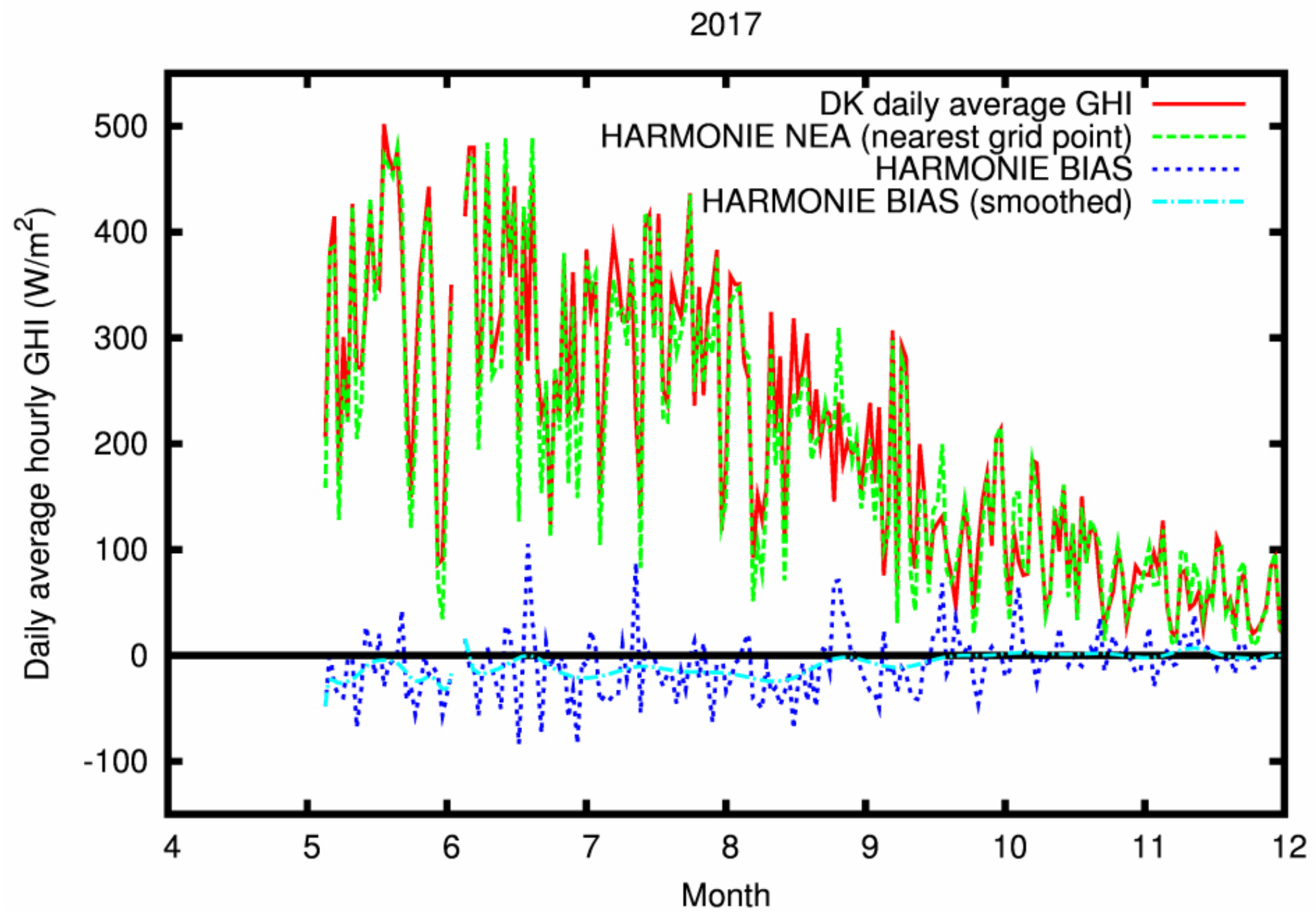
Figure 5.
Monthly mean bias (W/m−2) for (a) March (b) June (c) August and (d) October using observations and MÉRA data for the period 2008 to 2014.
Figure 5.
Monthly mean bias (W/m−2) for (a) March (b) June (c) August and (d) October using observations and MÉRA data for the period 2008 to 2014.
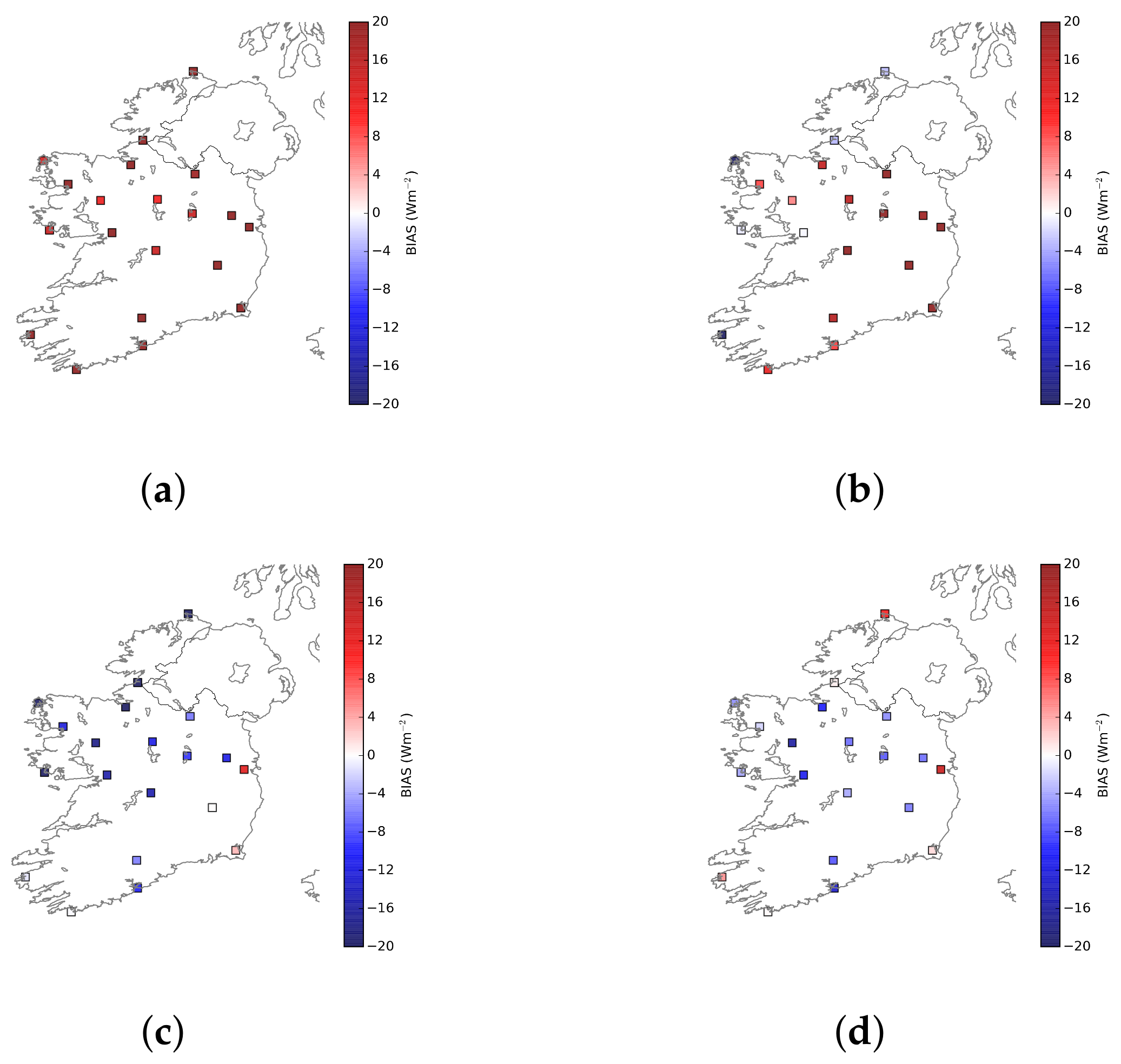
Figure 6.
Monthly mean RMSE. The colours show the RMSE scaled by monthly mean GHI (%) for (a) March (b) June (c) August and (d) October using observations and MÉRA data for the period 2008 to 2014. The RMSE in Wm−2 are marked on the plot.
Figure 6.
Monthly mean RMSE. The colours show the RMSE scaled by monthly mean GHI (%) for (a) March (b) June (c) August and (d) October using observations and MÉRA data for the period 2008 to 2014. The RMSE in Wm−2 are marked on the plot.

Figure 7.
Monthly mean biases in GHI per station in Denmark for the months of June, July, August and September in 2017. The colour shows the relative GHI bias with respect to the measured GHI.
Figure 7.
Monthly mean biases in GHI per station in Denmark for the months of June, July, August and September in 2017. The colour shows the relative GHI bias with respect to the measured GHI.
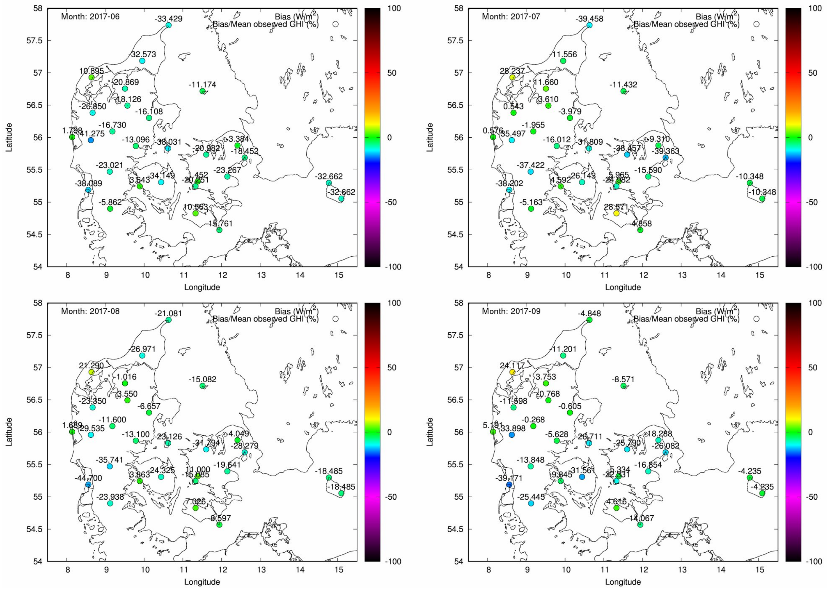
Figure 8.
Monthly mean RMSE per station in Denmark for the months of June, July, August and September in 2017. The colour shows the relative RMSE with respect to the measured GHI.
Figure 8.
Monthly mean RMSE per station in Denmark for the months of June, July, August and September in 2017. The colour shows the relative RMSE with respect to the measured GHI.

Figure 9.
Monthly mean observed (green curves) and modelled (red curves) GHI for each station in Denmark for the months of June, July, August and September in 2017, shown as graphs with the station numbers on the x-axis. Bias (blue curves) and RMSE (magenta curves) are also shown for each stations.
Figure 9.
Monthly mean observed (green curves) and modelled (red curves) GHI for each station in Denmark for the months of June, July, August and September in 2017, shown as graphs with the station numbers on the x-axis. Bias (blue curves) and RMSE (magenta curves) are also shown for each stations.
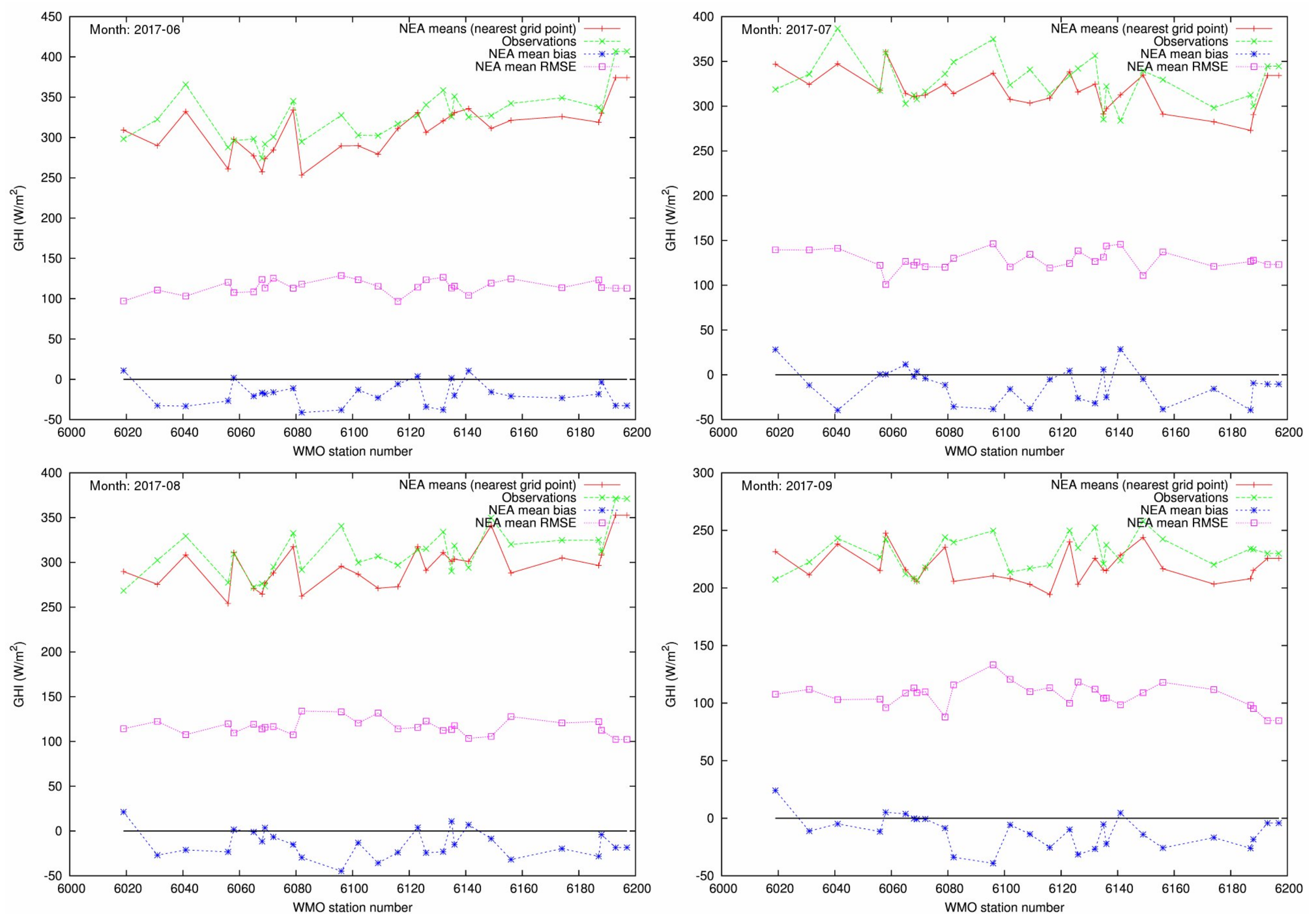
Figure 10.
Time series of daily mean clear sky index (CSI) (weighted using hourly GHI) averaged over the TUCSON stations. Thirty-day averaging is applied. Observations (red), MÉRA data (blue) and the bias in MÉRA relative to observations (green) are shown.
Figure 10.
Time series of daily mean clear sky index (CSI) (weighted using hourly GHI) averaged over the TUCSON stations. Thirty-day averaging is applied. Observations (red), MÉRA data (blue) and the bias in MÉRA relative to observations (green) are shown.
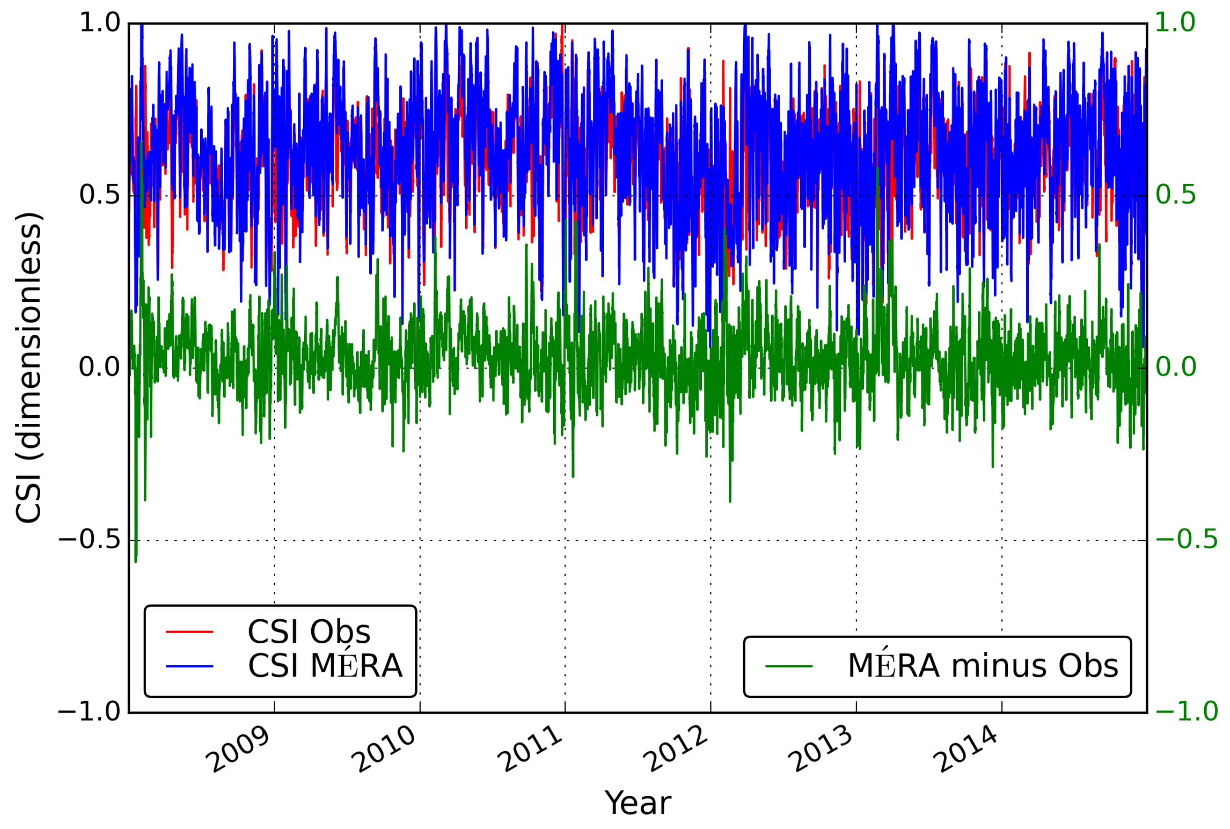
Figure 11.
Frequency distribution of daily mean CSI (weighted using hourly SW irradiance) for observations and MÉRA data using data for the period 2008 to 2014.
Figure 11.
Frequency distribution of daily mean CSI (weighted using hourly SW irradiance) for observations and MÉRA data using data for the period 2008 to 2014.
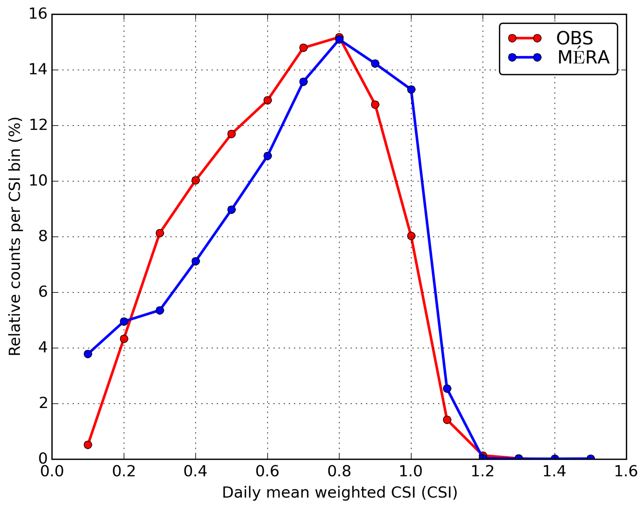
Figure 12.
Frequency distribution of daily mean CSI (weighted using hourly SW irradiance) for observations and Danish NEA data (May to December 2017).
Figure 12.
Frequency distribution of daily mean CSI (weighted using hourly SW irradiance) for observations and Danish NEA data (May to December 2017).

Figure 13.
Time series of daily variability index averaged over all Irish TUCSON stations. Thirty-day averaging is applied. Observations, MÉRA data and the bias in MÉRA relative to observations are shown. Data for the period 2008 to 2014 are included.
Figure 13.
Time series of daily variability index averaged over all Irish TUCSON stations. Thirty-day averaging is applied. Observations, MÉRA data and the bias in MÉRA relative to observations are shown. Data for the period 2008 to 2014 are included.
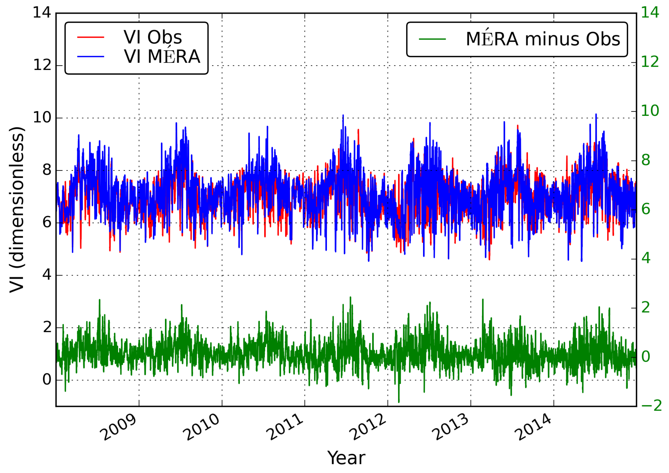
Figure 14.
Frequency distributions for MÉRA of daily weighted CSI for the following variability index (VI) bins (a) 0 to 5, (b) 5 to 10, (c) 10 to 15 using data for the period 2008 to 2014.
Figure 14.
Frequency distributions for MÉRA of daily weighted CSI for the following variability index (VI) bins (a) 0 to 5, (b) 5 to 10, (c) 10 to 15 using data for the period 2008 to 2014.

Figure 15.
2D histograms of the binned Danish HARMONIE-AROME NEA CSI values as a function of the observed CSI values for the month of June 2017. The results are divided into four VI bins with the ranges: upper left, VI 0 to 5; upper right, VI 5 to 7.5; lower left, VI 7.5 to 10; lower right, VI 10 to 15.

Table 1.
HARMONIE-AROME configuration used for MÉRA. SYNOP, synoptic station .
| Model Version | HARMONIE-AROME 38h1.2 |
| Domain | 540 × 500 grid points ( 2.5 km) |
| Vertical Levels | 65 levels up to 10 hPa, first level at approximately 12 m |
| Forecast Cycle | 3 h |
| Data Assimilation | Optimal interpolation for surface parameters |
| 3DVAR assimilation for upper air parameters | |
| Observations | Pressure from SYNOP, SHIP and DRIBU |
| Temperature and winds from AIREP and AMDAR | |
| Winds from PILOT | |
| Temperature, winds and humidity from TEMP | |
| Forecast | 3-h forecasts, but a 33-h forecast at 00 Z |
Table 2.
HARMONIE-AROME configuration used for the Danish Meteorological Institute (DMI) Northern Europe A (NEA) domain.
Table 2.
HARMONIE-AROME configuration used for the Danish Meteorological Institute (DMI) Northern Europe A (NEA) domain.
| Model Version | HARMONIE-AROME 40h1.1 |
| Domain | 1280 × 1080 grid points ( 2.5 km) |
| Vertical Levels | 65 levels up to 10 hPa, first level at approximately 12 m |
| Forecast Cycle | 3 h |
| Data Assimilation | Optimal interpolation for surface parameters |
| 3DVAR assimilation for upper air parameters | |
| Observations | Pressure from SYNOP, SHIP and DRIBU |
| Temperature and winds from AIREP, AMDAR and MODE-S-EHS | |
| Radiances from AMSU-A, MHS and ATMS | |
| Atmospheric Motion Vectors (AMV) from MSG | |
| GNSS-RO bending angles from Metop-A, Metop-B and COSMIC | |
| Radar volume data from OPERA | |
| Winds from PILOT | |
| Temperature, winds and humidity from TEMP | |
| Forecast | 60-h forecasts |
© 2018 by the authors. Licensee MDPI, Basel, Switzerland. This article is an open access article distributed under the terms and conditions of the Creative Commons Attribution (CC BY) license (http://creativecommons.org/licenses/by/4.0/).
Share and Cite
MDPI and ACS Style
Nielsen, K.P.; Gleeson, E. Using Shortwave Radiation to Evaluate the HARMONIE-AROME Weather Model. Atmosphere 2018, 9, 163. https://doi.org/10.3390/atmos9050163
AMA Style
Nielsen KP, Gleeson E. Using Shortwave Radiation to Evaluate the HARMONIE-AROME Weather Model. Atmosphere. 2018; 9(5):163. https://doi.org/10.3390/atmos9050163
Chicago/Turabian StyleNielsen, Kristian Pagh, and Emily Gleeson. 2018. "Using Shortwave Radiation to Evaluate the HARMONIE-AROME Weather Model" Atmosphere 9, no. 5: 163. https://doi.org/10.3390/atmos9050163
Note that from the first issue of 2016, this journal uses article numbers instead of page numbers. See further details here.