Article

PM2.5 Characteristics and Regional Transport Contribution in Five Cities in Southern North China Plain, During 2013–2015

1
State Key Laboratory of Atmospheric Boundary Layer Physics and Atmospheric Chemistry, Institute of Atmospheric Physics, Chinese Academy of Sciences, Beijing 100029, China
2
University of Chinese Academy of Sciences, Beijing 100049, China
3
Laboratory of Critical Zone Evolution, School of Earth Sciences, China University of Geosciences, Wuhan 430074, China
4
Department of Chemistry, Analytical and Testing Center, Capital Normal University, Beijing 100048, China
5
Hebei Province Meteorological Observatory, Shijiazhuang 050022, China
*
Author to whom correspondence should be addressed.
Atmosphere 2018, 9(4), 157; https://doi.org/10.3390/atmos9040157
Submission received: 4 March 2018 / Revised: 3 April 2018 / Accepted: 12 April 2018 / Published: 21 April 2018
(This article belongs to the Special Issue Air Quality in China: Past, Present and Future)

Abstract

:
PM2.5 data from major cities in the southern North China Plain during 2013–2015 were comprehensively analyzed relative to variation features, meteorology effects, and regional transport contributions. The annual average ranged from 87 to 123 μg m−3, with the highest in Baoding and Shijiazhuang, the moderate in Handan and Hengshui, and the lowest in Cangzhou, which revealed an evident concentration gradient with distance from the mountains. PM2.5 pollution indicated significantly regional characteristics and high correlations in daily PM2.5 changes and similar seasonal and diurnal variations in five cities. The highest concentrations mainly occurred in the winter, then autumn, spring, and summer, and the diurnal variations were bimodal with peaks during the morning rush hours and at night, which were mostly dominated by the differences in source emissions and the boundary layer. The PM2.5 concentrations were significantly positively correlated with relative humidity, especially during winter. The highest PM2.5 concentrations in all cities were associated with the south, southeast, and southwest pathways, while the short northwest pathway in the winter for Baoding and Shijiazhuang experienced the highest concentration. Regional contributions ranged from 19.6 to 33.7% annually, with the largest in Baoding and Shijiazhuang. These results provide a scientific basis for pollution forecasting and control in these heavily polluted cities.

1. Introduction

Haze pollution in the southern Hebei province of the North China plain has deteriorated in recent decades [1,2,3]. The highest PM2.5 particles with aerodynamic diameters ≤2.5 μm levels in this region have been reported recently [4,5,6] and can result in severe health risks. Rapid growth in both the economy and energy consumption, especially in coal combustion, industrialization, urbanization, and motorization, together with a unique topography, which is surrounded by mountains to the north and west (Figure 1a) [7,8,9,10], have contributed to this heavy pollution. The aerosol pollution in this region has been investigated by several studies using analyses of chemical compositions [11,12,13] and a source apportionment that uses air quality models [14,15,16]. These studies have shown that high level emissions of gaseous precursors (NOx, SO2, and VOCs etc.) and high concentrations of secondary inorganic ions, organic carbon, elemental carbon, and most crustal elements, together with unique local topographic factors and unfavorable meteorological conditions contributed to higher PM2.5 concentration. Overall, coal combustion, industrial and domestic sources, and regional transport were the major contributors to the severe pollution levels in this region [10]. The main industries and enterprises (power plants and heavy industries etc.) emitting exhaust gases in Hebei Province and the population distribution are shown in Figure 1b,e.
To mitigate the haze pollution, the most comprehensive and strict national action plan for air pollution prevention and control was proposed by China’s State Council on 10 September 2013. The PM2.5 levels in the Beijing-Tianjin-Hebei region are required to drop 25% in 2017 compared to 2012 levels. Accordingly, a strict action plan for air pollution prevention and control was also released by the government of the Hebei province (Available online: http://www.hebei.gov.cn/). A series of emission reduction measures, including the optimization and adjustment of the industrial structure, industrial air pollution control, the management of coal quality and usage, vehicle fuel quality and emission control, and dust control were implemented. However, Shijiazhuang (SJZ, the provincial capital of Hebei), Baoding (BD), Handan (HD), and Hengshui (HS) were ranked in the top 10 most polluted cities in China from 2013 to 2015 by the Ministry of Environmental Protection of China (MEPC) (Available online: http://www.zhb.gov.cn/xxgk/jjwm/index_1.shtml). Thus, improving air quality in these cities is both necessary and urgent.
Previous studies have focused on short-term pollution episodes [17,18] or pollution conditions only in SJZ [4,12], which has not aided in understanding the long-term annual, seasonal, and diurnal variation of PM2.5 in major cities in the southern Hebei province. This lack of information hinders the research of physical and chemical processes that affect the air quality. Additionally, regional transport is under the control of atmospheric circulation patterns and this is a significant contribution to PM2.5 pollution levels in the heavily polluted surrounding areas [10,19]. Massive studies have reported the significant influence of the southern Hebei province on Beijing air pollution [19,20,21]. However, the regional transport contributions in the major cities of southern Hebei are rarely investigated and they urgently need to be studied and quantified for each heavily polluted city. It is critical to understand and establish the emission reduction strategy at the local and regional scales [21].
In this paper, the annual, seasonal, and diurnal variations of PM2.5 concentrations, as well as the influence of the meteorological conditions in the five major cities of southern Hebei were analyzed from 2013 to 2015. The transport pathways and contributions from the surrounding regions were also explored using receptor models, such as potential source contribution function analysis [22,23] and trajectory sector analysis [21,24], by combining the observed PM2.5 concentrations and back trajectories. This information will be crucial for improving the understanding of pollution formation mechanisms, enhancing the forecast accuracy, and developing effective pollution control strategies in this most polluted region.

2. Data and Methodology

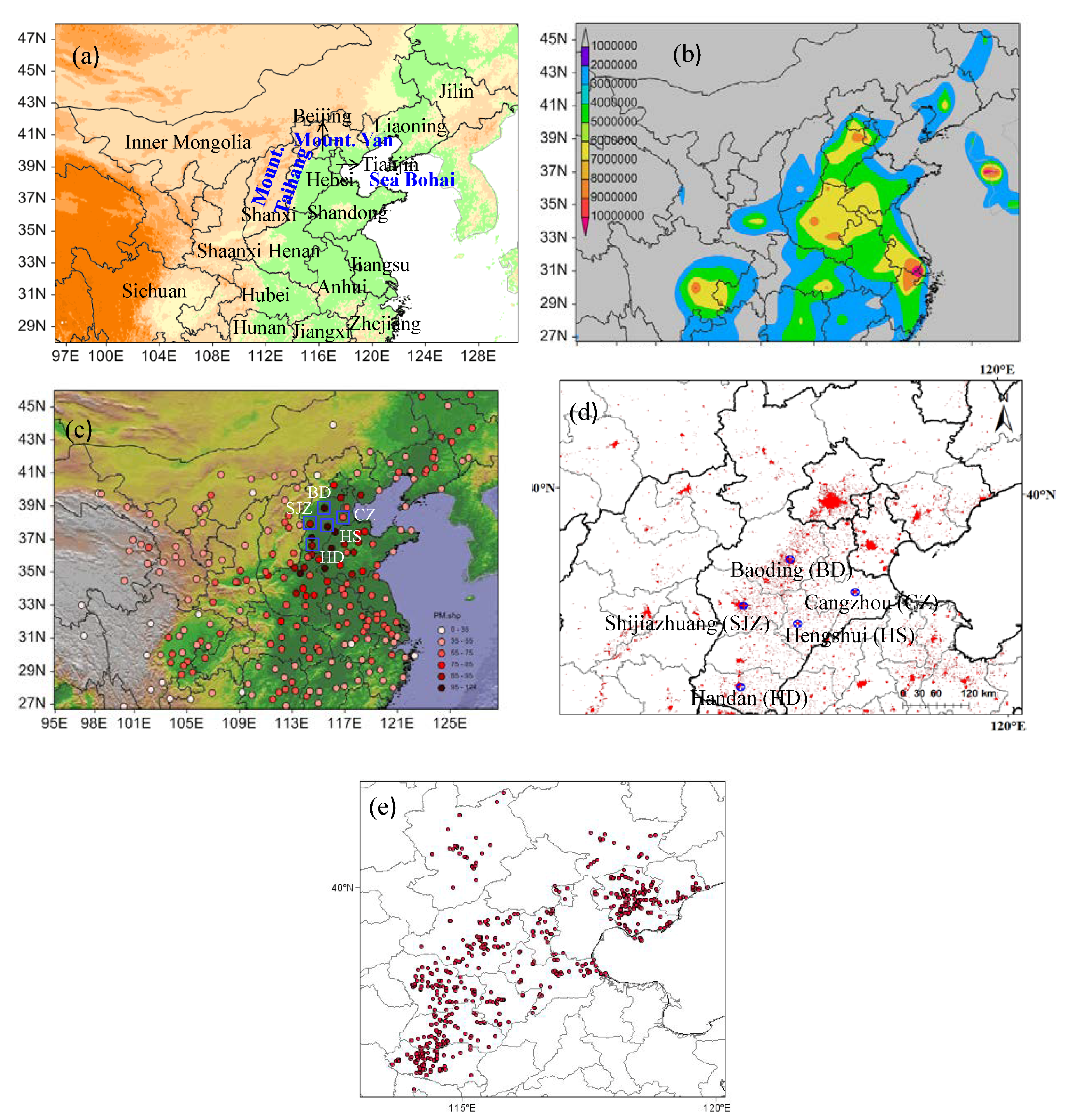
2.1. Description of the Study Cities

Hebei province, which includes 11 prefectural-level cities, is located in North China, with the mountains to the north and west, oceans to the east, and the plains to the south (Figure 1a). Hebei province and the municipalities of Beijing and Tianjin are merged as the Jing-Jin-Ji city cluster region, which has one of the largest populations globally (Figure 1b). The gross domestic product (GDP) of Hebei is 2942.12 billion RMB, and coal consumption is 296.35 million tons, which puts it in sixth and fourth place, respectively, out of 31 provinces and municipalities in China according to the China Statistical Yearbook 2014. In addition, the fraction of secondary industry in this region (e.g., heavy industry, real estate) accounts for 51.05% in all three industries. The climate in Hebei province is characterized by a continental monsoon zone that has a prevailing northerly wind with dry, cold air and little precipitation in winter and a prevailing southerly wind with wet, hot air and high precipitation in summer and transitional periods in spring and autumn. The 5 prefectural cities, SJZ, BD, HD, HS, and Cangzhou (CZ) (Figure 1d), are located in the southern Hebei province and had populations of 10.03, 10.29, 9.38, 4.42, and 7.38 million people (4.30, 2.81, 1.65, 0.52, and 0.47 million in the urban area), and GDPs of 510.0, 275.78, 308.00, 113.9, and 313.34 billion RMB, respectively, based on the Hebei Statistical Yearbook 2014. In addition, vehicle counts were 2.19, 2.13, 1.63, 0.89 and 1.47 million until the second quarter of 2015 (Available online: http://www.hetj.gov.cn/). The highest PM2.5 concentrations in China were observed in this region in 2015 (Figure 1c).

2.2. PM2.5 and Meteorological Data

The real-time, hourly PM2.5 concentration data were downloaded from the live-updated website published by the MEPC (Available online: http://www.zhb.gov.cn/) during 2013–2015. All monitoring sites were located in the urban areas of the cities. There were four sites in BD, five sites in SJZ, three sites in HD, three sites in HS, and three sites in CZ. The hourly data of concentrations from these monitoring sites in every city were averaged over three hours, six hours, and daily for further analysis, with at least 18 hourly values required calculating the daily averages. PM2.5 was measured using a micro oscillating balance method from commercial instruments according to the China Environmental Protection Standards HJ 655-2013 (Available online: http://kjs.mep.gov.cn/hjbhbz/).
Every 6-h interval meteorological parameters (local time 02:00, 08:00, 14:00, 20:00) during 2013–2015 in the five cities (Figure S1) were acquired from the China Meteorological Administration. Daily temperature (T), wind speed (WS), relative humidity (RH), and precipitation were averaged using the four measurement results. Six-hour interval wind directions (WD) and WS, as well as six-hour averaged PM2.5 concentrations were used to plot the maps of wind rose and the relationship between PM2.5, WS, and WD.
The planetary boundary layer heights (PBLH) in 3-h intervals were obtained from the U.S. National Oceanic and Atmospheric Administration (NOAA) READY archived meteorological GDAS data (1° × 1°) (Available online: http://www.ready.noaa.gov/READYamet.php) based on Coordinated Universal Time (UTC). All UTC values were converted to local time (Beijing time).

2.3. Backward Trajectory Modeling

The HYSPLIT4.9 model from the (NOAA) Air Resources Laboratory (Available online: http://ready.arl.noaa.gov/HYSPLIT.php) and meteorological data (GDAS for 1° × 1° resolution) were used to calculate the individual, three-day backward trajectories. The trajectory endpoint was the city center at a height of 200 m above ground level (i.e., within the mixed layer). The city centers were located in BD at 38.89° N and 115.49° E, SJZ at 38.05° N, and 114.54° E, HD at 36.60° N and 114.52° E, HS at 37.74° N and 115.68°E, and CZ at 38.32° N and 116.87° E). The backward trajectories were calculated at 00:00, 03:00, 06:00, 09:00, 12:00, 15:00, 18:00, and 21:00 UTC every day for each city during 2013–2015 in five cities. Three-hour averaged PM2.5 concentrations before the end time of each trajectory were combined with the backward trajectories and used for the trajectory cluster and receptor models.

2.4. Methods

2.4.1. Trajectory Cluster Method

To explore the impact of air mass transport on PM2.5 pollution in the target cities, backward trajectories were clustered based on Euclidean distance and a suitable cluster number was determined using the ‘eye ball’ method with the software TrajStat [25]. PM2.5 concentrations were grouped according to the trajectory cluster. Normalized contributions for the different clusters to PM2.5 concentrations were calculated on an annual and seasonal basis by combining the occurring frequency of every cluster and the responding PM2.5 averaged concentrations.

2.4.2. Potential Source Contribution Function (PSCF) and Trajectory Sector Analysis (TSA) Method

To investigate and quantify the effect of regional transport on PM2.5 concentrations in a receptor city, the receptor models of the PSCF [26] and TSA [10,24] were used. Both are based on the results of the HYSPLIT model and PM2.5 concentrations. The domain zone of the PSCF is divided into i × j small equal grid cells with a 0.5° × 0.5° resolution. The domain zone and the threshold values for the five cities during the study period are shown in Table S1. The total number of trajectory endpoints in the ijth grid cell is nij and the total number of trajectory endpoints for which the measured pollutant concentration exceeds a threshold value is mij. The PSCF value in the ijth cell is defined as mij/nij. In this study, the 75% percentile value was chosen as the threshold, which represented the heavy pollution criterion. To remove the uncertainty in cells with small nij values, such as those less than approximately three times the average number of trajectory endpoints in all the i × j cells, a weight function W(nij) was adopted as follows based on running the PSCF program many times,
W ( n i j ) =   { 1.00   ( 150 < n i j )   0.70   ( 50 < n i j 150 ) 0.42   ( 20 < n i j 50 ) 0.17   ( n i j 20 )    
The TSA method first divided into twelve 30° sectors in the central of the receptor city, numbered in a clockwise direction (1–12) starting in the north. To reduce the converting deviation, the analysis region was fixed in the range of 28–60° N and 70–130° E. The locations of the trajectory during the first 4 h were excluded because the sectors might be poorly defined close to the origin, and a small amount of curvature in a trajectory can lead to spurious results [24]. The average concentration of sector j (Cj) and the percentage of the concentration associated with air masses from sector j (%Cj) are defined by i = 1 N C i f i j / N j and C j N j / j = 1 12 C j N j × 100 , respectively. N is the total number of trajectories, Ci is the concentration within the ith trajectory, fij is the time spent in sector j for the ith trajectory, and Nj ( i = 1 N f i j ) is the total time during which the trajectories passed through sector j. The detailed information about the trajectory cluster, PSCF and TSA methods are described in Wang et al., 2015 [10].

3. Results and Discussion

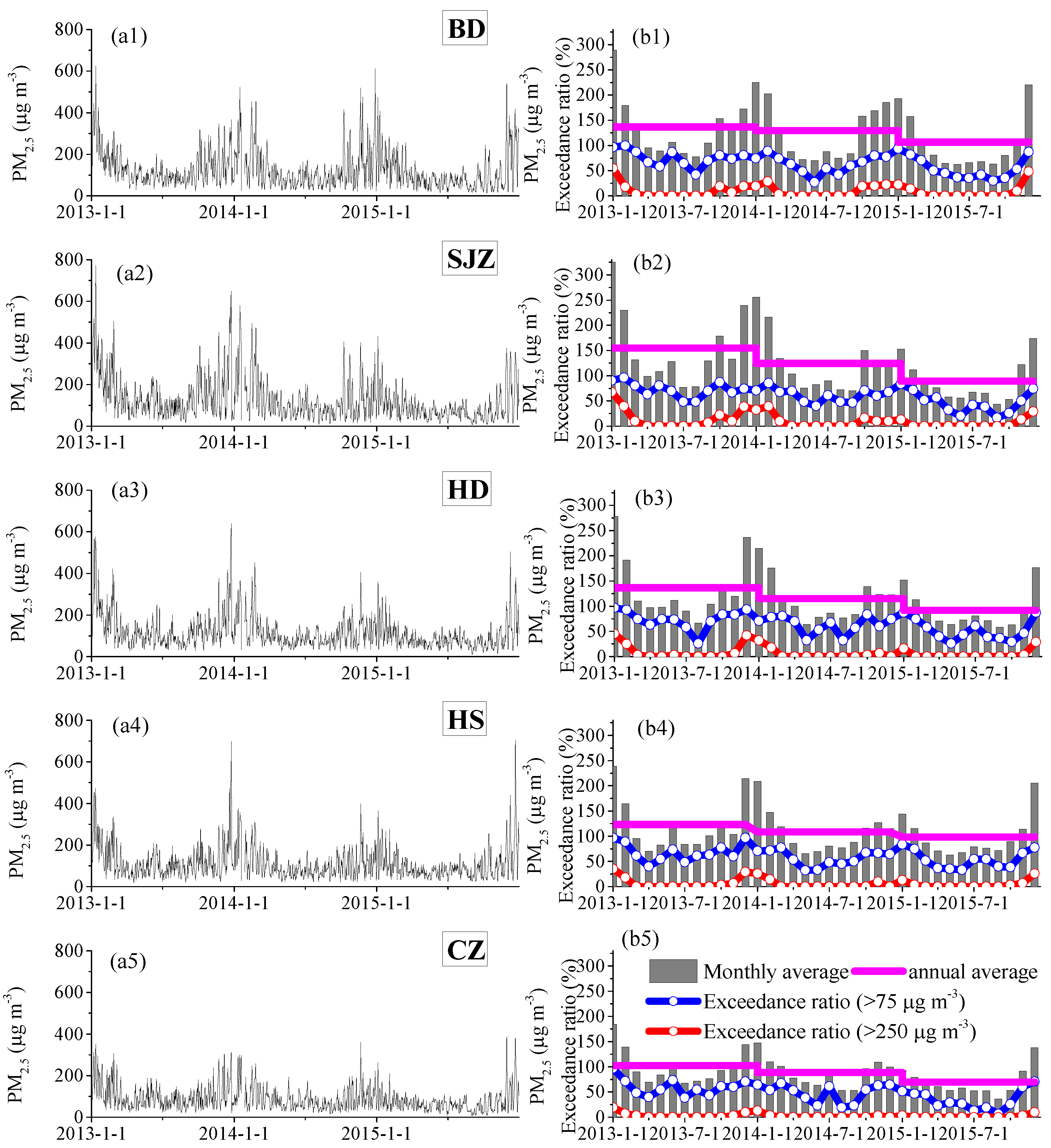
3.1. Characteristics of PM2.5 Concentrations in Five Cities during 2013–2015

3.1.1. Overview of the PM2.5 Concentrations

The annual average PM2.5 concentrations during 2013–2015 were 123 ± 90, 122 ± 101, 114 ± 81, 109 ± 77, and 87 ± 58 μg m−3 for BD, SJZ, HD, HS, and CZ, respectively (Table 1), which severely exceeded the Chinese Ambient Air Quality Standards (CAAQS) Grade I (yearly limit 15 μg m−3) by 6–8 times and Grade II (yearly limit 35 μg m−3) by 2.5–3.5 times. The population-weighted mean of PM2.5 in all five cities was 119 μg m−3, which was six times as high as the global population-weighted mean (20 μg m−3) [27] and highlighted a high health risk. It is important to note that the annual PM2.5 concentrations in BD, SJZ, HD, and HS were much higher than those in other Chinese cities that have been reported previously [4,7]. The maximum daily average PM2.5 concentrations were 626, 771, 641, 705, and 387 μg m−3 in BD, SJZ, HD, HS, and CZ, respectively (Figure 2a), all of which occurred during winter and indicated extreme fine particle pollution. In general, the ratio at which PM2.5 exceeded 75 μg m−3, the daily limit for Grade II CAAQS, was between 48.1–64.9%, and the ratio at which PM2.5 > 250 μg m−3, the threshold value for the most severe pollution, was between 2.2–10.2%. The most severely polluted cities were located near the mountains including BD, SJZ, and HD, while the less-polluted cities were located near the sea, like CZ. This is attributed to adverse diffusion conditions with the orographic wind convergence zones along the Taihang and Yanshan Mountains [18] and the lower PBLH (Figure 3). The severe pollution levels in this region are caused by both local primary emissions from industrial and domestic sources and secondary production from the abundant precursors [10,12,13,15,28,29], as well as the special topography (Figure 1a), the unfavorable weather conditions that are stagnant with weak winds and low PBLH (Figure 3 and Figure 4), and the regional transport contribution [10,15,18,21].
The day-to-day variations of PM2.5 in these cites (Figure 2a) showed similar trends, and the concentrations were elevated synchronously in all cities during heavy haze episodes, largely driven by the evolution of synoptic circulation and meteorological factors. The correlation coefficients between the daily PM2.5 concentrations in the cites were 0.74–0.88 (Table 1), which demonstrated the regional fine particulate pollution characteristic due to the horizontal and vertical homogeneity of the meteorological conditions in the study region (Figure 3 and Figure 4) and the secondary formation of PM2.5 [30]. The annual average PM2.5 concentrations from 2013 to 2015 in these cities declined significantly each year (Figure 2b). The annual average values in 2013 were in the range of 103–155 μg m−3, but decreased by 30–66 μg m−3 in 2015 and ranged from 70 to 107 μg m−3, with a reduction in the differences among the cities as well. The largest decline was observed in SJZ, from 155 in 2013 to 89 μg m−3 in 2015. The rapid decline of PM2.5 annual means was partially ascribed to the decreased frequency of extremely heavy pollution incidences because of the exceedance ratio at which PM2.5 > 250 μg m−3 (Figure 2) dropped from 3.6–16.2% in 2013 to 1.4–8.2% in 2015. Furthermore, the largest reduction occurred during winter, declining by 24, 119, 88, 51, and 53 μg m−3 in BD, SJZ, HD, HS, and CZ, respectively, between 2013 and 2015. This was the season that contributed the most to the decrease in annual mean PM2.5. The meteorological conditions became slightly unfavorable from 2013 to 2015, with weakening winds, especially in SJZ in 2014, and decreasing humidity, with the exception of autumn (Figure 4). The precursors of PM2.5 (like NO2 and SO2) in North China also significantly declined from 2013 to 2015, which was observed from OMI satellite (Figure S2). Thus, the effectiveness of source reduction measures in this region was significant and facilitated the decline of PM2.5 concentrations. Remarkably, the even stricter environmental protection laws were enforced in China beginning on 1 January 2015 (http://www.gov.cn/xinwen/2014-04/25/content_2666328.htm), which could further the implementation of pollution control measures.

3.1.2. Seasonal Variation

The seasonal and monthly average PM2.5 concentrations are shown in Table 1 and Figure 2. At least 20 daily mean concentrations were required to calculate the monthly averages. Seasonal categories are divided into spring (March, April, and May), summer (June, July, and August), fall (September, October, and November), and winter (December, January, and February). The annual variation in monthly averaged PM2.5 concentrations showed similar seasonal trends during 2013–2015. In general, the highest concentrations of PM2.5 were observed in the winter (126–203 μg m−3), followed by autumn (79–118 μg m−3), spring (82–98 μg m−3), and summer (67–82 μg m−3), successively. Additionally, the differences in PM2.5 concentrations between the cities peaked in winter and were lowest in summer. The PM2.5 pollution levels in CZ were not as severe as the other cities, which had higher ratios of attaining the CAAQS Grade II (32.3–63.4%) in all four seasons. In the other 4 cities, attainment days were less than 20% in winter and severely polluted days (PM2.5 concentration > 250 μg m−3) accounted for 19.0–30.8%. Additionally, the attainment ratios in spring and autumn were in the range of 37.1–50.5%, and the highest attainment ratios were in summer at 49.6–53.5%.
The highest PM2.5 concentrations almost always occurred during the winter months in the study cities. The most polluted month on record was January 2013, which was caused by extremely unfavorable weather conditions and high secondary transformation, as previously reported [10,16,18,31]. The spring PM2.5 maxima usually occurred in March and the autumn maxima in November or October, due to the increased emissions from domestic heating and agricultural burning during the October harvest season [10,32,33]. The variations in emissions, meteorological conditions, type of long-distance transport, and secondary production are associated with the pollution levels in different seasons [34]. The highest density of coal consumption and heavy industries are also found in this region, which emitted massive primary particles and gaseous precursors [29,35]. The highest concentrations were found in winter and autumn due to the enhanced anthropogenic emissions from coal combustion for heating and biomass burning for the clean-up of agricultural waste [36]. Stagnant meteorological conditions often occurred in winter and autumn with less precipitation, moderate humidity (average 62%) (Figure 3), lower PBLH (average 320 m) (Figure 4), and higher frequencies of weak winds (Figure 5), which together suppressed pollution diffusion and facilitated particle production and hygroscopic growth. Although the warm temperature and high humidity during summer promoted the photochemical formation of particles, the lower emissions and higher precipitation resulted in the lowest PM2.5 concentrations. The highest wind speeds and PBLH occurred during spring and facilitated air ventilation and vertical convection, resulting in lower pollution levels. The regional transport influence will be discussed in Section 3.3 and Section 3.4.

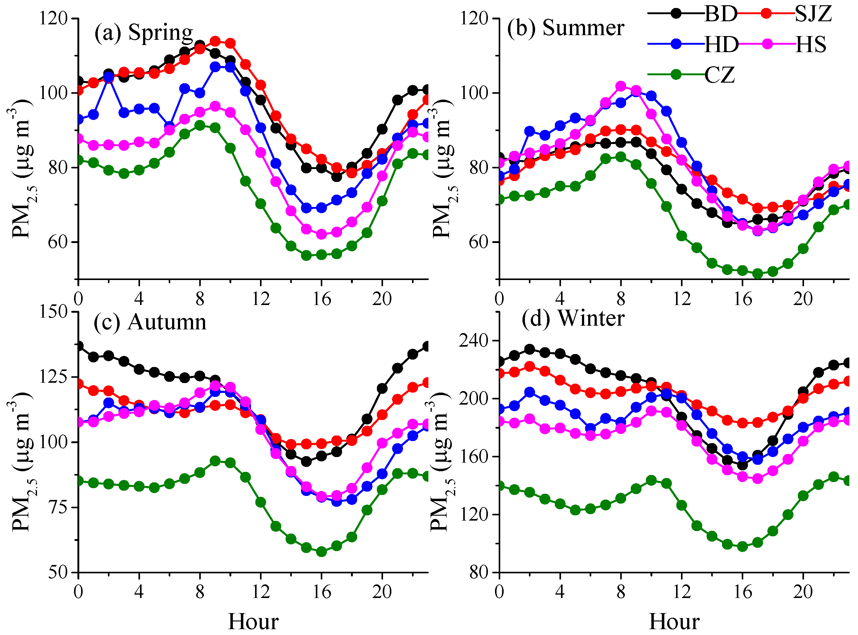
3.1.3. Diurnal Variation

The seasonal diurnal variation of PM2.5 in all the study cities during 2013–2015 is shown in Figure 6 to identify the potential emission sources. A bimodal pattern with peaks during the morning rush hours (e.g., traffic exhausts) and at night was observed. The morning peak during autumn and winter was approximately 1–2 h later compared to that in spring and summer (8–9 a.m.), due to the low PBLH before noon (Figure 3). The decreased afternoon concentrations were attributed to the better dispersion conditions, with increasing PBLH and wind speeds. From 1600 to the nighttime, the afternoon rush hours and increased source activities caused an increase PM2.5 concentration, while the declining PBLH after sunset resulted in pollution accumulation. The highest PM2.5 concentrations in all cities occurred during winter and autumn. Furthermore, the concentrations at night were higher than during the day. This was associated with the enhanced emissions from domestic heating and the lower PBLH. The best air quality occurred during the summer due to good diffusion conditions and less anthropogenic emissions, with minimum concentrations during the afternoon between 52 and 69 μg m−3, which also exceeded the CAAQS Grade II The highest concentrations were observed in SJZ and BD, except during summer, and the lowest were observed in CZ. This can be explained by the higher emissions from industrial and residential sources [15,35] and more stagnant atmosphere with lower PBLH in SJZ and BD. However, during summertime, the highest concentrations occurred in HD and HS. One possible explanation are the weak winds and the higher frequency of southerly winds (Figure 2a).

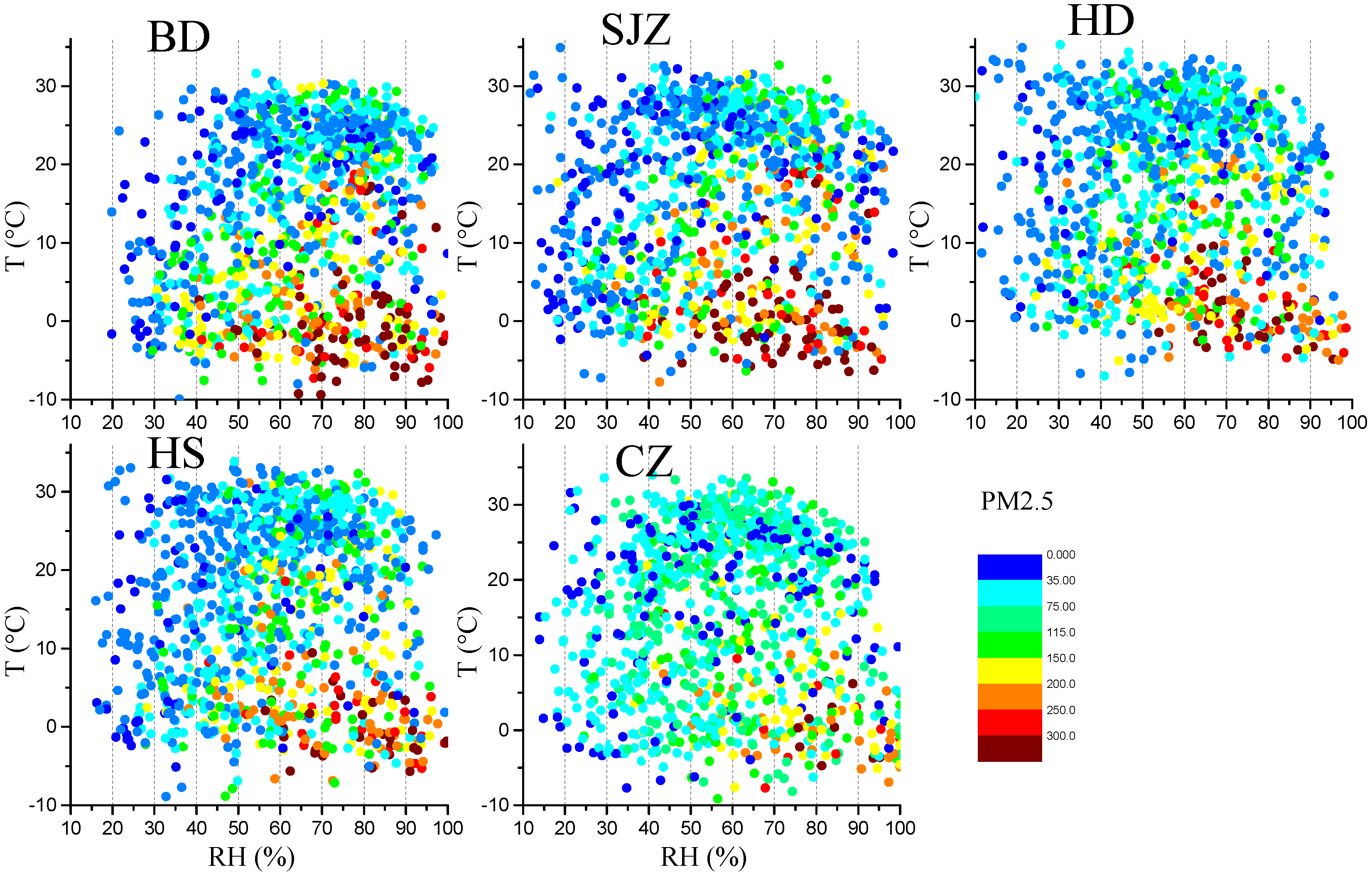
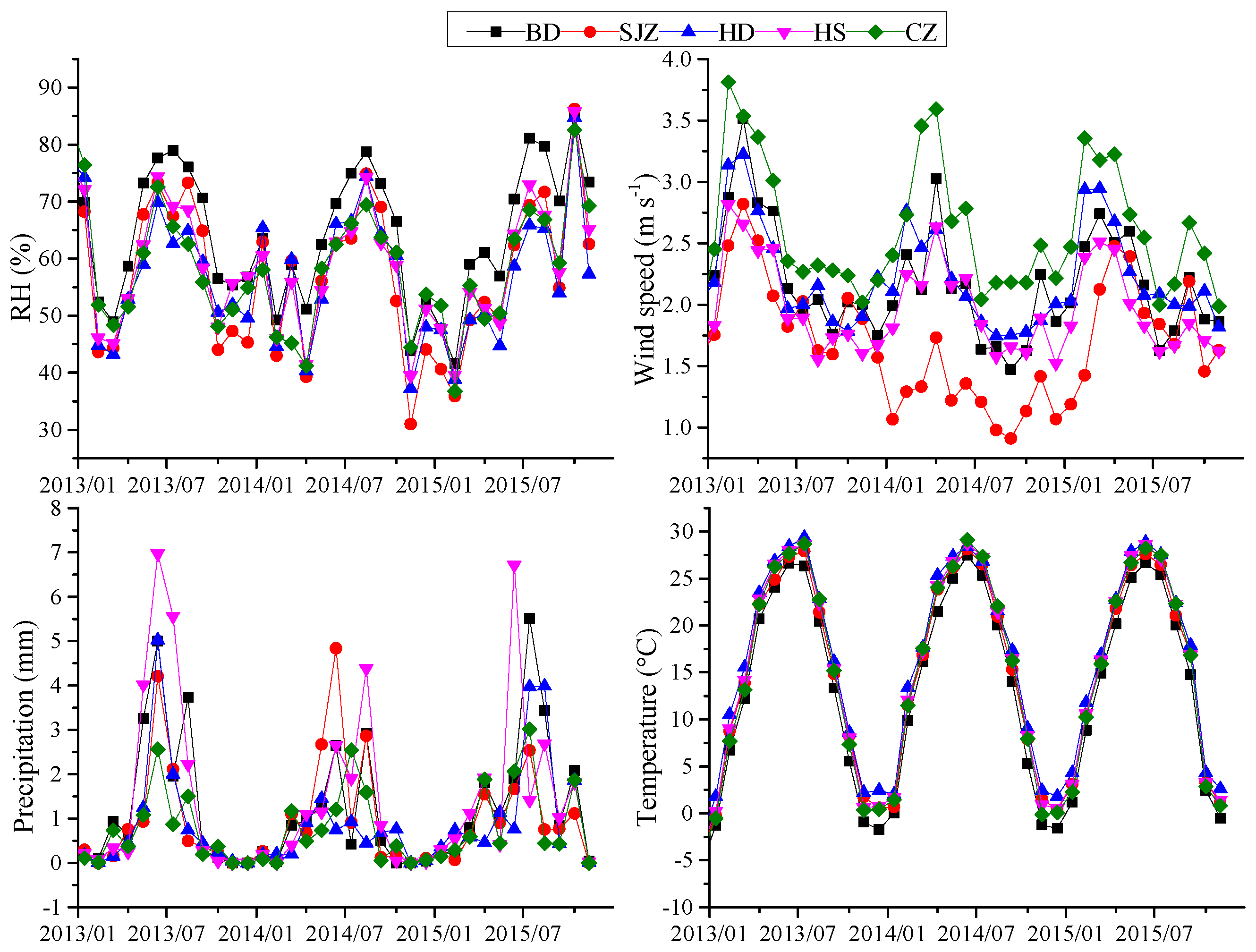
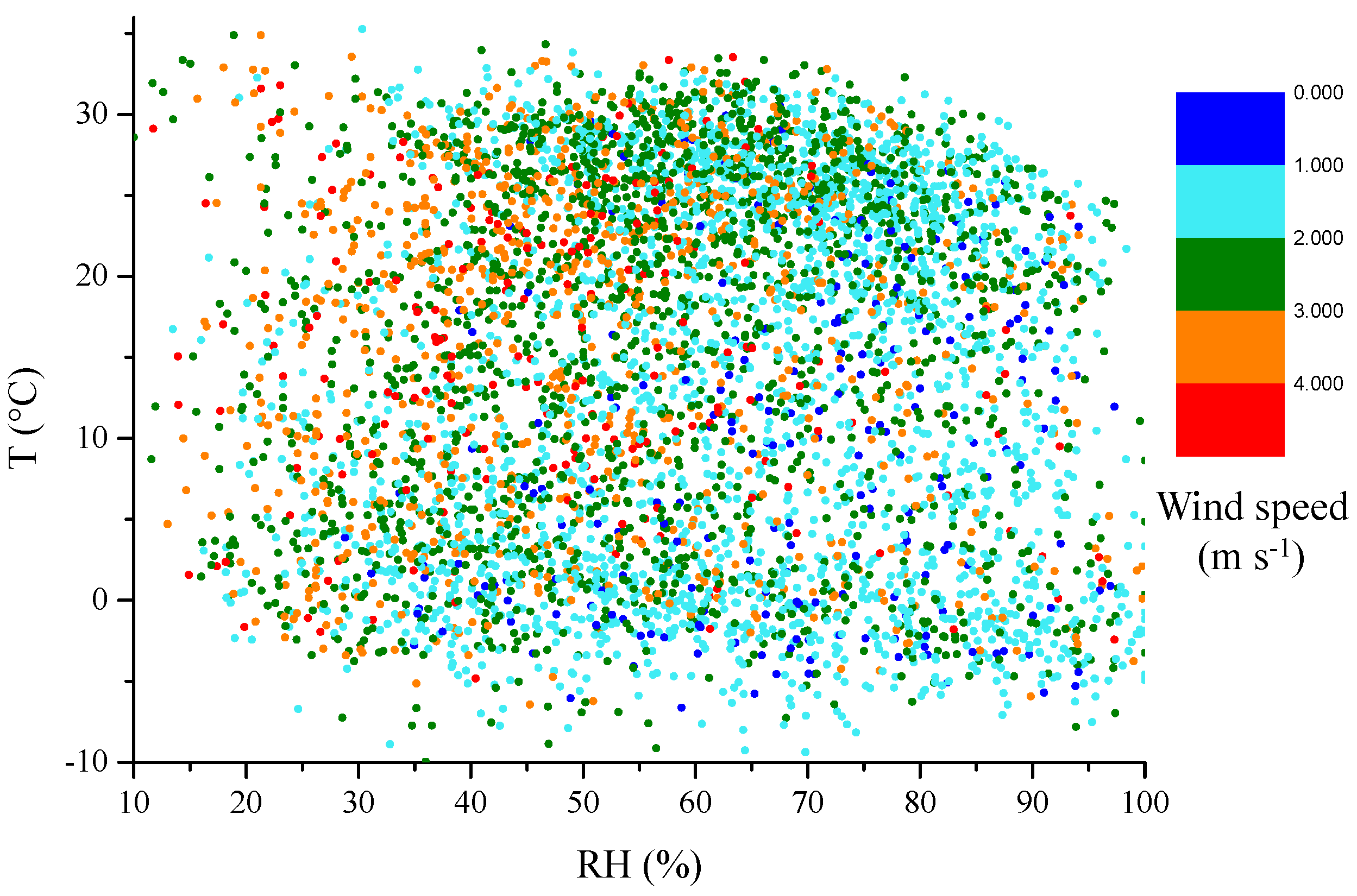
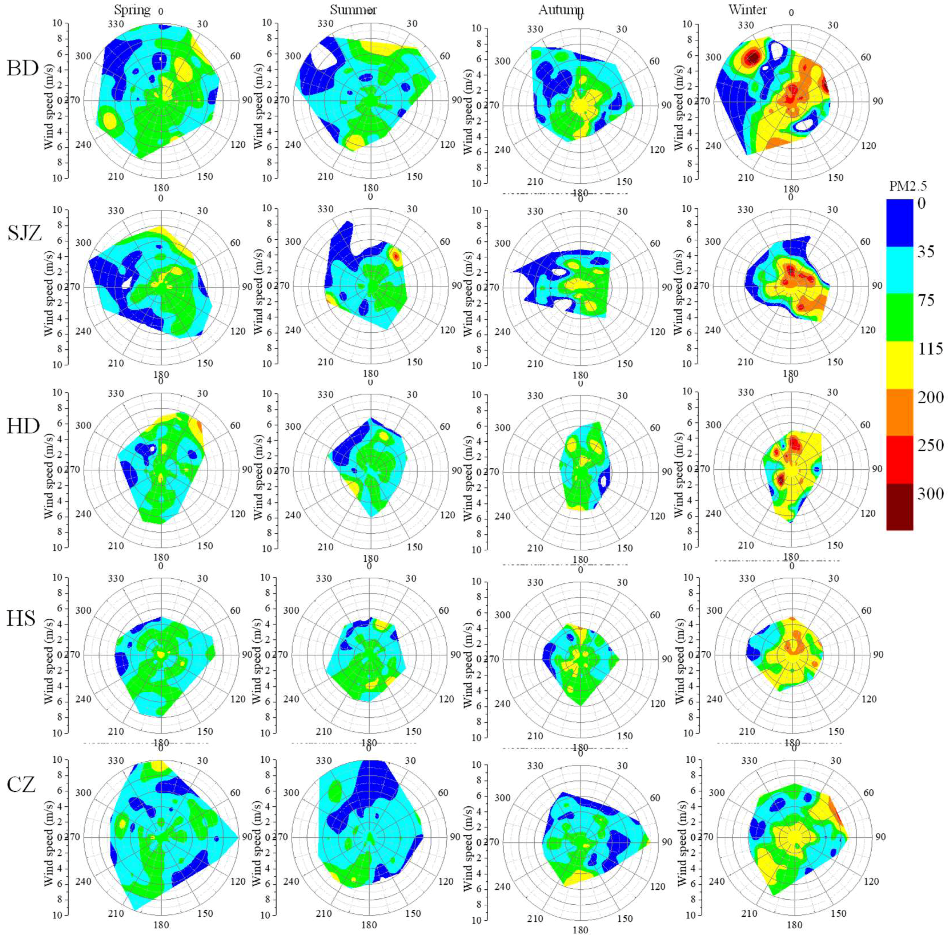
3.2. Relationship between PM2.5 and Meteorological Parameters

The relationship between pollutants and meteorological factors in the five study cities during 2013–2015 was quantified into four seasons using Pearson correlation coefficients (Table 2). In general, the correlation coefficients of the cities showed little difference, indicative of the regional pollution characteristic. A negative correlation between the PM2.5 and WS (wind speed) was observed, especially in winter, which suggested that horizontal dispersion was important. However, a weak correlation in summer was likely due to a higher PBLH, which promoted vertical dilution. Weak negative correlations were observed between PM2.5 and precipitation in the same day or the previous day, while these correlations were not significant in most cities. The positive correlation between PM2.5 and temperature was only observed in the summer, which indicated that the photochemical reaction was important during that time, whereas, the negative correlations in other seasons were likely associated with higher emissions from heating or the condensation of semi-volatile species in low temperatures. It should be noted that these correlations were not significant in half of the study cities.
PM2.5 concentrations were significantly positively correlated with RH during all seasons and in all cities, with stronger correlations during winter. Weak correlations in summer and autumn were ascribed to massive precipitations in summer and early autumn, which contributed to higher humidity and eliminated particles through wet deposit. The RH- and T-dependent distribution of PM2.5 and wind speed (Figure 7 and Figure 8) demonstrated an obvious concentration gradient with the elevated RH. On average, the lowest PM2.5 concentrations occurred at RH < 30% with no dependence on T, which was likely due to the ability of the high winds to disperse the pollutants. The PM2.5 showed a rapid increase when RH > 50%, especially at low temperatures. These results illustrated that severe haze events in this region mostly occurred in conditions of high humidity, weak winds, and high emissions due to heating in cold periods. High humidity plays an important role in elevating pollution levels by facilitating particle transformation, hygroscopic growth [31,37] and the partition of semi-volatile species into the aerosol phase [38], meanwhile high humidity usually accompanies lower PBLH [39].
The PM2.5 concentrations of target cities are not only decided by local emissions, but also by the surrounding pollution regions. Maps of wind rose and the relationships between the 6-h average PM2.5 concentration, wind speed, and wind direction in the study cities are presented in Figure 5 and Figure 9 to investigate the regional influence. The lowest wind speeds were found in SJZ, HD, and HS, epically during winter and autumn. The wind speeds associated with southeasterly to southwesterly winds were usually very low, except for HD, HS, and CZ in spring and summer. The strong northwesterly winds were mostly in BD and only occurred during summer in SJZ and CZ. At the remaining sites, northwesterly winds were weak. High PM2.5 values were associated with weak winds, less than 2 m s−1, which revealed higher local emissions. Low PM2.5 values were associated with winds from the northwest except during winter. In most cities, PM2.5 concentration increased with elevated wind speed in different wind directions, which is indicative of the influence of the regional transport from the surrounding polluted regions. The regional transport is discussed in detail in the next sections.

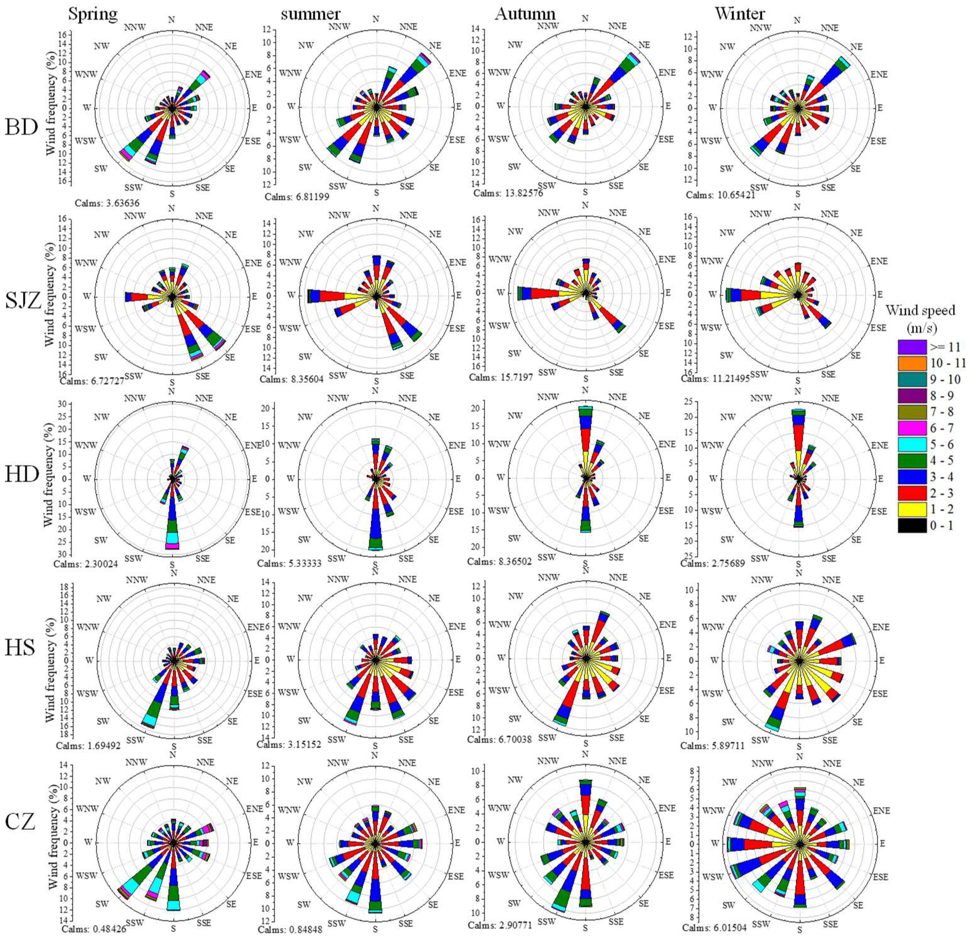
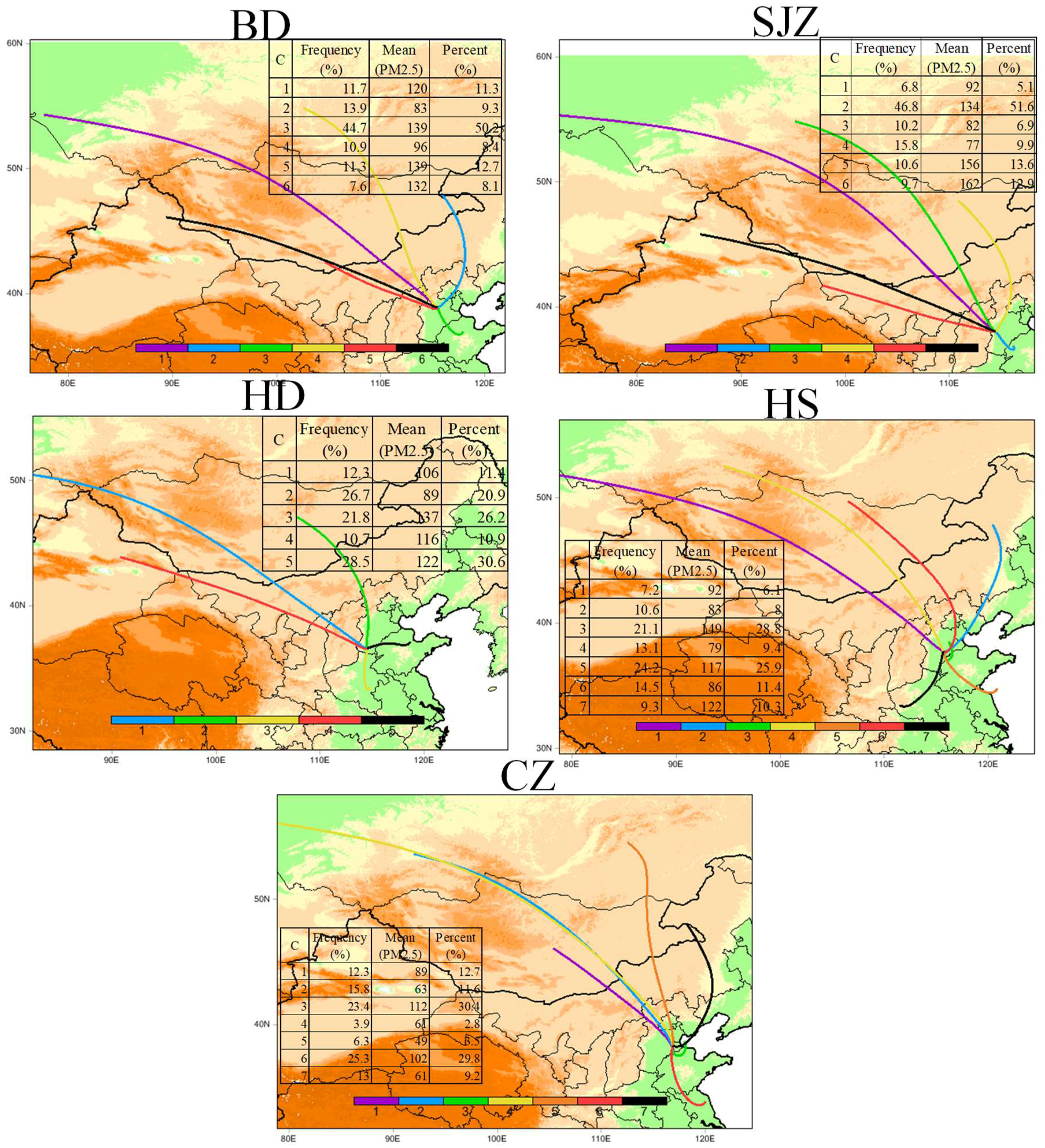
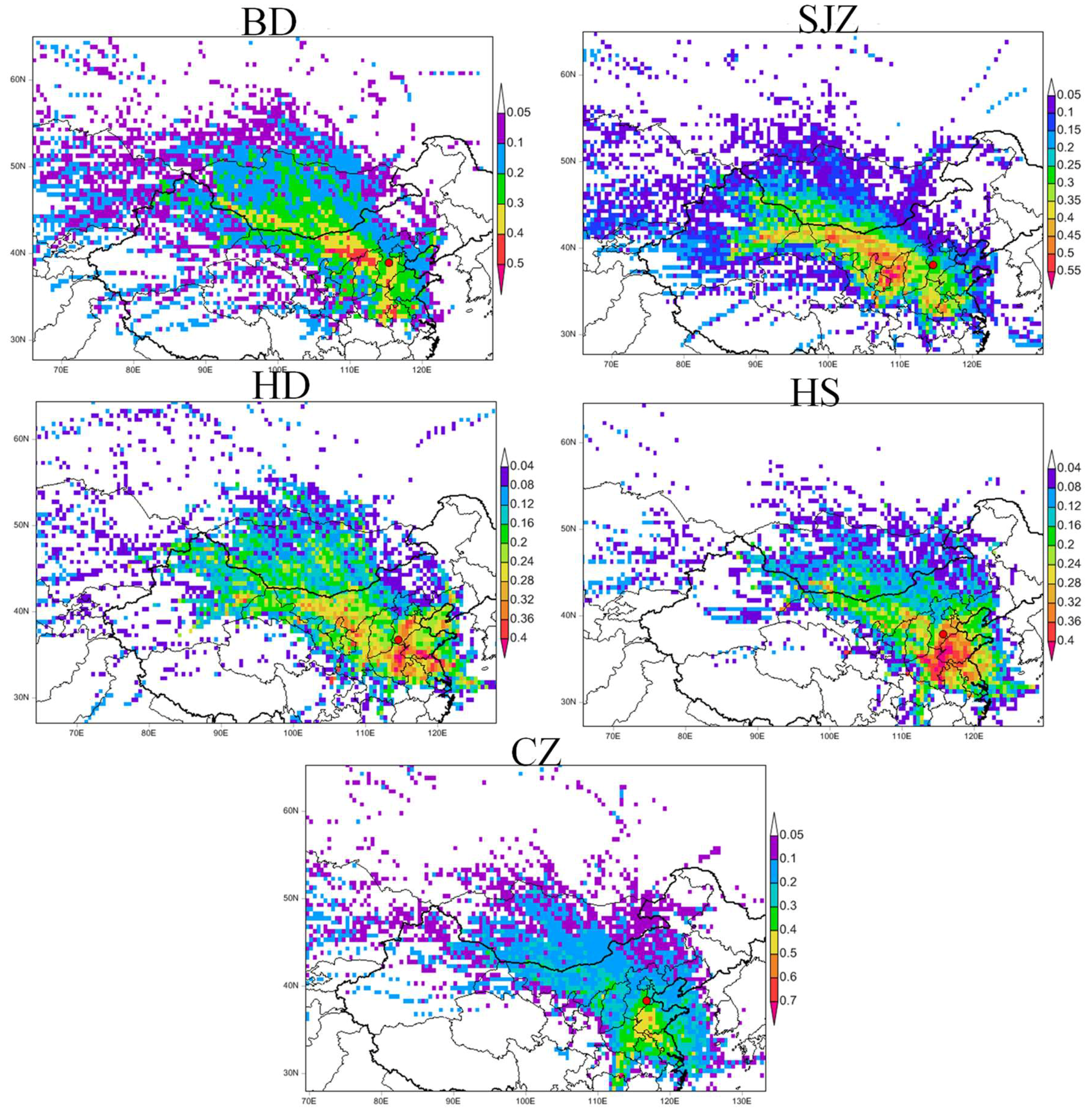
3.3. Transport Pathways and Source Analysis

The main transport pathways, corresponding PM2.5 concentrations, and normalized contributions to PM2.5 concentrations as defined by the cluster frequency and the mean PM2.5 concentration in all cities for the entire study period and different seasons are displayed in Figure 10 and Figure S3. The main transport pathways can be divided into seven categories from the results of the trajectory clusters: north (N; BD-C2, SJZ-C4, HD-C2, HS-C2, CZ-C5 & C7), long northwest (NWL; BD-C1 & C4, SJZ-C1 & C3, HD-C1, HS-C1 & C4, CZ-C2 & C4), short northwest (NWS; BD-C5 & C6, SJZ-C5 & C6, HD-C4, CZ-C1), long southeast (SEL; BD-C3, SJZ-C2, HD-C5, HS-C5), short southeast (SES; HS-C3, CZ-C3), south (S; HD-C3, CZ-C6), and southwest (SW; HS-C7). The southernly pathways, SEL, SES, S, and SW, were predominant and accounted for 44.7%, 46.8%, 50.3%, 54.6%, and 48.7%, respectively, in BD, SJZ, HD, HS, and CZ. NWS pathways made larger contributions of 18.9–20.3% in BD and SJZ, and less than 12.3% in other cities. In addition, due to the monsoonal influence, the frequency of southern pathways increased in the summer, and northern pathways increased in the winter.
The highest PM2.5 concentrations were generally associated with NWs, SEL SES, S, and SW pathways in the range of 132–139 μg m−3 for BD, 134–162 μg m−3 for SJZ, 116–137 μg m−3 for HD, 117–149 μg m−3 for HS, and 89–112 μg m−3 for CZ, which was higher than the corresponding annual averaged concentrations. Moderate PM2.5 concentrations (46–67 μg m−3) were associated with the NWL, and the lowest PM2.5 concentrations (20~33 μg m−3) with the N. On the seasonal scale, mean PM2.5 concentrations for different pathways showed somewhat similar trends, but the magnitudes in the same cluster varied according to season, with the highest concentrations in winter and lowest in summer. Moreover, the PM2.5 concentrations associated with the southerly pathways were higher than those associated with the NWS for seasonal means. Due to the high occurrence frequency of the southerly pathways, as well as their high corresponding PM2.5 concentrations, the southerly pathways contributed the most to PM2.5 concentrations on the order of 50.2–65.0% for all cities. The seasonal PM2.5 contributions from every pathway also changed, with increased contributions from the southerly pathways during the summer and decreased contributions during the winter. Notably, the NWS pathways in winter were large contributors to PM2.5 in BD and SJZ, at 25.8% and 38.2%.
The potential source contributions to the high PM2.5 concentrations varied among the cities (Figure 11). These results suggested that regional transport from the northwest and south of BD and SJZ played a dominant role in the formation of severe haze pollution events. These regions included southwestern Inner Mongolia, northern Shanxi and Shannxi, southern Hebei, eastern Henan, western Shandong, and northern Anhui and Jiangsu. The high potential source regions for HS were located in southern Hebei, Shandong, Henan, and northern Jiangsu and Anhui. Remarkably, the domain of potential sources was the largest in HD and smallest in CZ. The high PSCF values for HD were located in western Inner Mongolia, northern Shannxi, southern Shanxi and Hebei, Tianjin, eastern and central of Henan, western and southern Shandong, and northern Jiangsu and Anhui. The high PSCF values for CZ were in southern Hebei, Shandong, eastern and central of Henan, northern Anhui and Jiangsu, and central Hubei.
Generally, the contribution from the surrounding areas was consistent with the distributions of the source emissions. A huge amount of anthropogenic emissions from industrial production, vehicle exhaust, and domestic sources cover the surrounding regions in the study cities [35]. For example, coal mining, power generation regions, numerous metallurgical works, and coal chemical industries are located in Shanxi and southwestern Inner Mongolia, which emit lots of particles and gaseous precursors. Domestic heating with coal in the winter leads to higher emissions of pollutants. Moreover, stagnant weather with weak winds is often accompanied by the southerly winds, which brings pollutants into the cities, especially near the mountains, inducing the elevated pollution levels.

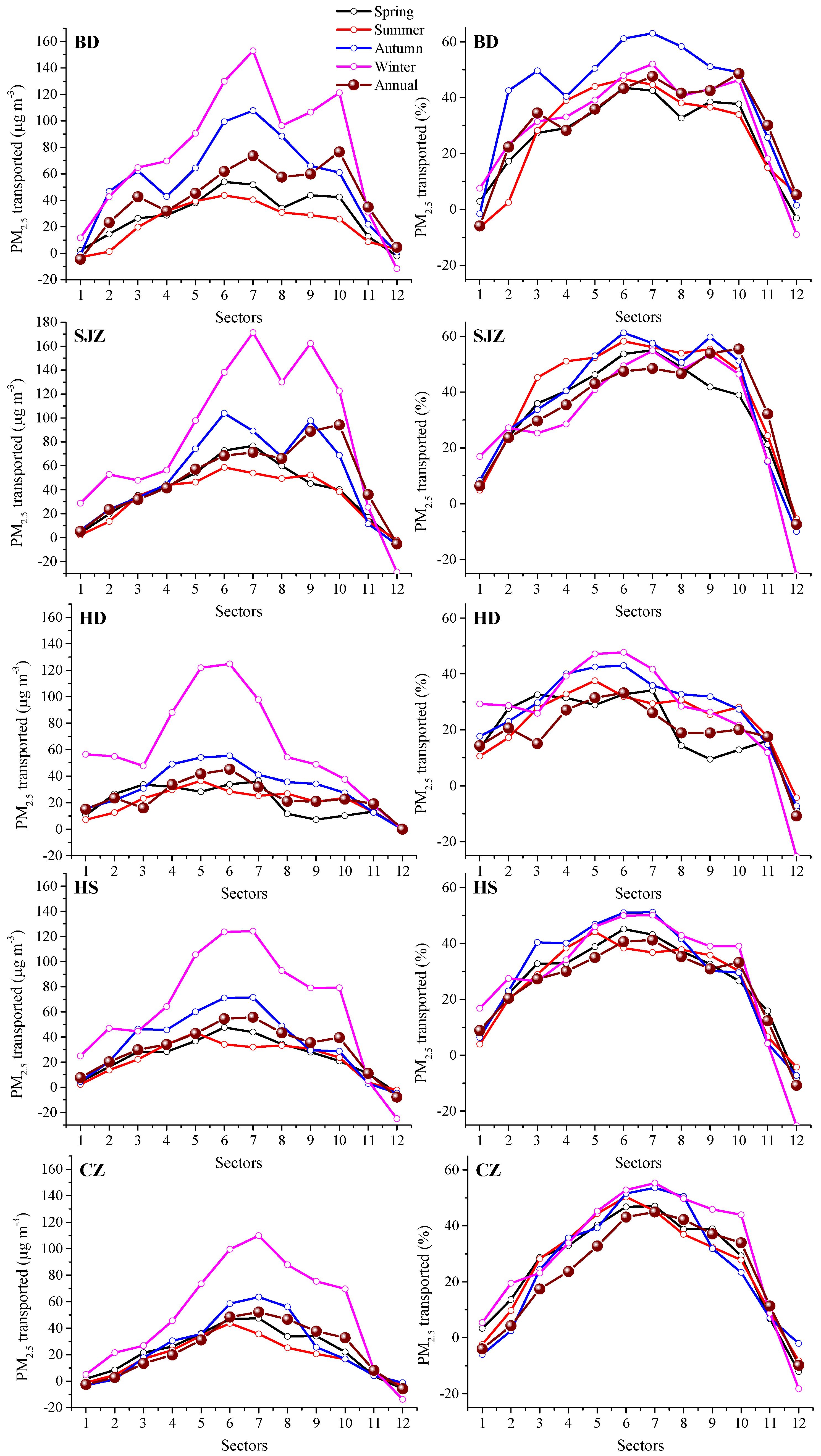
3.4. Regional Transport Contribution

According to the TSA method, annual and seasonal 12 sector concentrations (Cj) and percentages (%Cj) of PM2.5 in the study cities are presented in Figure S4, which demonstrated evident sector gradients. On average, with the exception of HD, the highest mean concentrations of PM2.5 (ranging from 138–170 μg m−3 in BD and SJZ, and 97–135 μg m−3 in HS and CZ) were associated with sectors 6–10, moderate mean concentrations with sectors 2–5 and 11, and the smallest mean concentrations (ranging from 58–87 μg m−3) in sectors 1 and 12. The highest concentrations of PM2.5 were in sectors 4–6 in HD, ranging from 124–136 μg m−3, and the lowest concentrations in sector 12 (91 μg m−3). The concentration gradients of the trajectory sectors in BD and SJZ were larger than those in HD, HS, and CZ, which indicated there were more contributions from regional transport to PM2.5 pollution levels in BD and SJZ. The seasonal variation in sector concentrations exhibited similar trends to the annual variation in all cities. However, the concentrations in all sectors were highest in winter, while sectors 5–7 had the highest summer concentrations. The sector concentration percentages were highest in sectors 6–7 and 10–11 for BD and SJZ, sectors 1–3, 5–7, and 10–12 for HD, and sectors 6–7 for HS and CZ. In addition, the increased sector percentages came from the southerly sectors during the summer and the westerly sectors during the winter due to the transition in the predominant wind direction.
The background and long-distance regional transported PM2.5 concentrations in the study cities were roughly estimated using the methods of Wang et al. (2015). The sectors with the lowest concentration were defined as the background concentration (Cb) due to the relatively few sources there. The locations of the trajectory during the first 4 h (Figure S5) represented the local extents, which was not resolved in the TSA analysis. The Cb levels of PM2.5 were 81 μg m−3 in sectors 1 and 12, 76 μg m−3 in sectors 1 and 12, 91 μg m−3 in sector 12, 80 μg m−3 in sectors 1 and 12, and 64 μg m−3 in sector 1, 11 and 12 for BD, SJZ, HD, HS, and CZ, respectively. Additionally, the Cb concentrations were highest in the winter and lowest in the summer. Figure 12 shows the annual and seasonal concentrations and contributions of transport components to PM2.5 in each sector of the different cities after subtracting Cb. The largest transported concentration and contribution was associated with sectors 5–10 for BD and SJZ ranging from 36% to 56%, and sectors 5–8 for HD, HS, and CZ ranging from 18% to 45%. The larger contribution from sectors 9–10 to BD and SJZ occurred in winter and autumn due to increased coal combustion use for heating in the northwest regions. The highest transported contributions in every sector changed slightly with the seasonal transition, with the highest contributions from the northwest in the winter and from the south in the summer.
The annual and seasonally transported PM2.5 concentrations and percent contribution during 2013–2015 for the study cities are displayed in Table 3, calculated by combining the transported concentrations or contributions and the frequency of the trajectories in the corresponding sectors. The annual mean contributions of 31.4% (42.4 μg m−3), 33.7% (46.4 μg m−3), 19.6% (23.3 μg m−3), 24.8% (30.2 μg m−3), and 20.2% (21.6 μg m−3) for BD, SJZ, HD, HS, and CZ, respectively, were attributed to long-distance transportation from the upwind polluted regions. The seasonal mean transported contributions showed higher values in summer and autumn, and lower in spring and winter. One explanation for this pattern is that more stagnant weather occurred in winter; thus, local emissions are more dominant. These results are comparable to previous source analysis results. The regional transport contribution accounted for 23–30% in SJZ, according to the China National Environmental Monitoring Center (http://www.cnemc.cn/publish/totalWebSite/news/news_42659.html), based on chemical composition apportionment. The transport contribution in winter was approximately 25% and 26.8% for SJZ and HD, obtained using complex atmospheric chemical transport models [10].

4. Summary and Conclusions

This study investigated the annual, seasonal, and diurnal variations of PM2.5 concentrations, as well as meteorological effects and source analysis for the five major cities in southern Hebei located in the North China Plain. This information will help to better understand the current PM2.5 characteristics in this most polluted region and provide a basis for pollution forecasting and management. The PM2.5 concentrations during 2013–2015 in the five cities were very high and indicated the overall regional fine particulate pollution. The population-weighted mean of PM2.5 was 119 μg m−3 in five cities, which was six times as high as the global population-weighted mean. However, a significant decline in PM2.5, especially in winter, was observed in the study cities, indicating the effectiveness of source reduction measures in this region.
The highest PM2.5 concentrations were mainly observed in the winter (126–203 μg m−3), followed by autumn (79–118 μg m−3), spring (82–98 μg m−3), and summer (67–82 μg m−3). In winter, attainment days only less than 20%, and the severely polluted days were 19.0–30.8%. The diurnal variations in PM2.5 in this study showed a bimodal pattern, except in the winter, and the peak at night in the winter was the highest due to enhanced emissions from heating and the reduced PBLH. In addition, high concentrations of PM2.5 were usually associated with high relative humidity (RH > 50%), especially a rapid increase of PM2.5 with elevated RH at low temperatures.
The analysis of the transport contribution indicated that the southerly pathways yielded the greatest PM2.5 contributions, ranging between 50.2–65.0% in all cities, whereas the short northwesterly pathway was a high contributor to PM2.5 concentrations in BD and SJZ (25.8–38.2%) during winter. Overall, more regional contributions were in BD and SJZ at 31.4% and 33.7%, whereas less contributions from 19.6–24.8% for HD, HS, and CZ. The regional contribution was highest in summer and autumn, and lowest in winter and spring. The heaviest PM2.5 pollution in BD and SJZ was ascribed to weak winds, low PBLH, and larger regional transport contributions, as well as large source emissions.

Supplementary Materials

The following are available online at https://www.mdpi.com/2073-4433/9/4/157/s1, Figure S1: Locations of the observation sites (red for PM2.5 and blue for meteorological observation) and the prefectural boundary layer in 5 cities in the south of North China Plain, Figure S2: The annual average variations of the NO2 tropospheric column and SO2 column amounts (planetary boundary layer) from the OMI satellite during 2013-2015 in NC (34-40°N, 110-120°E). (These data based on OMI level 3 products (OMSO2e.003 and OMNO2d ) were provided by GES DISC (Goddard Earth Sciences Data and Information Services Center)), Figure S3: Statistical summary of cluster frequency, PM2.5 concentrations associated with different trajectory clusters, and normalized contribution for different clusters to PM2.5 concentration in 5 cities during 2013-2015 for different seasons, Figure S4: Annual and seasonal sector concentrations (Cj) and percentages (%Cj) for PM2.5 in 5 cities during 2013-2015, Figure S5: The locations of the trajectories during the first 4 hours in the 5 cities during 2013-2015, Table S1: The domain zone and the threshold values for 5 cities during 2013-2015.

Acknowledgments

This work was partially supported by the National Natural Science Foundation of China (No. 41505133) and the grant of National Key R&D Plan (Quantitative Relationship and Regulation Principle between Regional Oxidation Capacity of Atmospheric and Air Quality 2017YFC0210003). Special thanks to the National Earth System Science, Data Sharing Infrastructure, and National Science & Technology Infrastructure of China.

Author Contributions

Lili Wang wrote the paper and contributed the study design; Yuesi Wang refined the interpretations; Wenjie Li, Minghui Tao, Jinyuan Xin, and Ying Kang analyzed the data; Yang Sun, Tao Song, Xingru Li, and Nan Zhang contributed PM2.5 data and meteorological data in 5 cities.

Conflicts of Interest

The authors declare no conflict of interest.

References

  1. Fu, G.Q.; Xu, W.Y.; Yang, R.F.; Li, J.B.; Zhao, C.S. The distribution and trends of fog and haze in the North China Plain over the past 30 years. Atmos. Chem. Phys. 2014, 14, 11949–11958. [Google Scholar] [CrossRef] [Green Version]
  2. Quan, J.; Zhang, Q.; He, H.; Liu, J.; Huang, M.; Jin, H. Analysis of the formation of fog and haze in North China Plain (NCP). Atmos. Chem. Phys. 2011, 11, 8205–8214. [Google Scholar] [CrossRef]
  3. Tao, M.; Chen, L.; Wang, Z.; Wang, J.; Tao, J.; Wang, X. Did the widespread haze pollution over China increase during the last decade? A satellite view from space. Environ. Res. Lett. 2016, 11, 54019–54026. [Google Scholar] [CrossRef]
  4. Wang, Y.; Ying, Q.; Hu, J.; Zhang, H. Spatial and temporal variations of six criteria air pollutants in 31 provincial capital cities in China during 2013–2014. Environ. Int. 2014, 73, 413–422. [Google Scholar] [CrossRef] [PubMed]
  5. Zhang, Y.; Cao, F. Fine particulate matter (PM2.5) in China at a city level. Sci. Rep. 2015, 5, 14484. [Google Scholar] [CrossRef] [PubMed]
  6. Tao, M.; Chen, L.; Li, R.; Wang, L.; Wang, J.; Wang, Z.; Tang, G.; Tao, J. Spatial oscillation of the particle pollution in eastern China during winter: Implications for regional air quality and climate. Atmos. Environ. 2016, 144, 100–110. [Google Scholar] [CrossRef]
  7. Han, L.; Zhou, W.; Li, W. Increasing impact of urban fine particles (PM2.5) on areas surrounding Chinese cities. Sci. Rep. 2015, 5, 12467. [Google Scholar] [CrossRef] [PubMed]
  8. Hu, H.; Zhang, X.H.; Lin, L.L. The interactions between China’s economic growth, energy production and consumption and the related air emissions during 2000–2011. Ecol. Indic. 2014, 46, 38–51. [Google Scholar] [CrossRef]
  9. Sheehan, P.; Cheng, E.; English, A.; Sun, F. China’s response to the air pollution shock. Nat. Clim. Chang. 2014, 4, 306–309. [Google Scholar] [CrossRef]
  10. Wang, L.T.; Wei, Z.; Yang, J.; Zhang, Y.; Zhang, F.F.; Su, J.; Meng, C.C.; Zhang, Q. The 2013 severe haze over southern Hebei, China: Model evaluation, source apportionment, and policy implications. Atmos. Chem. Phys. 2014, 14, 3151–3173. [Google Scholar] [CrossRef] [Green Version]
  11. Zhang, X.Y.; Wang, J.Z.; Wang, Y.Q.; Liu, H.L.; Sun, J.Y.; Zhang, Y.M. Changes in chemical components of aerosol particles in different haze regions in China from 2006 to 2013 and contribution of meteorological factors. Atmos. Chem. Phys. 2015, 15, 12935–12952. [Google Scholar] [CrossRef]
  12. Zhao, P.S.; Dong, F.; He, D.; Zhao, X.J. Characteristics of concentrations and chemical compositions for PM2.5 in the region of Beijing, Tianjin, and Hebei, China. Atmos. Chem. Phys. 2013, 13, 4631–4644. [Google Scholar] [CrossRef]
  13. Zhao, X.; Zhao, P.; Xu, J.; Meng, W.; Pu, W.; Dong, F.; He, D.; Shi, Q. Analysis of a winter regional haze event and its formation mechanism in the North China Plain. Atmos. Chem. Phys. 2013, 13, 5685–5696. [Google Scholar] [CrossRef]
  14. Gao, M.; Carmichael, G.R.; Wang, Y.; Saide, P.E.; Yu, M.; Xin, J.; Liu, Z.; Wang, Z. Modeling study of the 2010 regional haze event in the North China Plain. Atmos. Chem. Phys. 2016, 16, 1673–1691. [Google Scholar] [CrossRef]
  15. Li, X.; Zhang, Q.; Zhang, Y.; Zheng, B.; Wang, K.; Chen, Y.; Timothy, J.W.; Han, W.; Shen, W.; Zhang, X.; He, K. Source contributions of urban PM2.5 in the Beijing–Tianjin–Hebei region: Changes between 2006 and 2013 and relative impacts of emissions and meteorology. Atmos. Environ. 2015, 123 Pt A, 229–239. [Google Scholar] [CrossRef]
  16. Wang, Y.; Yo, L.; Wang, L.; Liu, Z.; Ji, D.; Tang, G.; Zhang, J.; Sun, Y.; Hu, B.; Xin, J.Y. Mechanism for the formation of the January 2013 heavy haze pollution episode over central and eastern China. Sci. China Earth Sci. 2014, 57, 14–25. [Google Scholar] [CrossRef]
  17. Ji, D.; Wang, Y.; Wang, L.; Chen, L.; Hu, B.; Tang, G.; Xin, J.; Song, T.; Wen, T.; Sun, Y.; Pan, Y.; Liu, Z. Analysis of heavy pollution episodes in selected cities of northern China. Atmos. Environ. 2012, 50, 338–348. [Google Scholar] [CrossRef]
  18. Wang, L.; Zhang, N.; Liu, Z.; Sun, Y.; Ji, D.; Wang, Y. The Influence of Climate Factors, Meteorological Conditions, and Boundary-Layer Structure on Severe Haze Pollution in the Beijing-Tianjin-Hebei Region during January 2013. Adv. Meteorol. 2014, 2014, 1–14. [Google Scholar] [CrossRef]
  19. Li, P.; Yan, R.; Yu, S.; Wang, S.; Liu, W.; Bao, H. Reinstate regional transport of PM2.5 as a major cause of severe haze in Beijing. Proc. Natl. Acad. Sci. USA 2015, 112, E2739–E2740. [Google Scholar] [CrossRef] [PubMed]
  20. Sun, Y.L.; Wang, Z.F.; Du, W.; Zhang, Q.; Wang, Q.Q.; Fu, P.Q.; Pan, X.L.; Li, J.; Jayne, J.; Worsnop, D.R. Long-term real-time measurements of aerosol particle composition in Beijing, China: Seasonal variations, meteorological effects, and source analysis. Atmos. Chem. Phys. 2015, 15, 10149–10165. [Google Scholar] [CrossRef]
  21. Wang, L.; Liu, Z.; Sun, Y.; Ji, D.; Wang, Y. Long-range transport and regional sources of PM2.5 in Beijing based on long-term observations from 2005 to 2010. Atmos. Res. 2015, 157, 37–48. [Google Scholar] [CrossRef]
  22. Ashbaugh, L.L.; Malm, W.C.; Sadeh, W.Z. A residence time probability analysis of sulfur concentrations at Grand Canyon National Park. Atmos. Environ. 1985, 19, 1263–1270. [Google Scholar] [CrossRef]
  23. Muir, D.; Longhurst, J.W.S.; Tubb, A. Characterisation and quantification of the sources of PM10 during air pollution episodes in the UK. Sci. Total Environ. 2006, 358, 188–205. [Google Scholar] [CrossRef] [PubMed]
  24. Bari, A.; Dutkiewicz, V.A.; Judd, C.D.; Wilson, L.R.; Luttinger, D.; Husain, L. Regional sources of particulate sulfate, SO2, PM2.5, HCl, and HNO3, in New York, NY. Atmos. Environ. 2003, 37, 2837–2844. [Google Scholar] [CrossRef]
  25. Wang, Y.; Zhang, X.; Draxler, R.R. TrajStat: GIS-based software that uses various trajectory statistical analysis methods to identify potential sources from long-term air pollution measurement data. Environ. Model. Softw. 2009, 24, 938–939. [Google Scholar] [CrossRef]
  26. Polissar, A.; Hopke, P.; Paatero, P.; Kaufmann, Y.; Hall, D.; Bodhaine, B.; Dutton, E.G.; Harris, J.M. The aerosol at Barrow, Alaska: Long-term trends and source locations. Atmos. Environ. 1999, 33, 2441–2458. [Google Scholar] [CrossRef]
  27. Van Donkelaar, A.; Martin, R.V.; Brauer, M.; Kahn, R.; Levy, R.; Verduzco, C.; Villeneuve, P.J. Global Estimates of Ambient Fine Particulate Matter Concentrations from Satellite-Based Aerosol Optical Depth: Development and Application. Environ. Health Persp. 2010, 118, 847–855. [Google Scholar] [CrossRef] [PubMed]
  28. Huang, R.J.; Zhang, Y.; Bozzetti, C.; Ho, K.F.; Cao, J.J.; Han, Y.M.; Daellenbach, K.R.; Slowik, J.G.; Platt, S.M.; Canonaco, F.; et al. High secondary aerosol contribution to particulate pollution during haze events in China. Nature 2014, 514, 218–222. [Google Scholar] [CrossRef] [PubMed] [Green Version]
  29. Krotkov, N.A.; McLinden, C.A.; Li, C.; Lamsal, L.N.; Celarier, E.A.; Marchenko, S.V.; Swartz, W.H.; Bucsela, E.J.; Joiner, J.; Duncan, B.N.; et al. Aura OMI observations of regional SO2 and NO2 pollution changes from 2005 to 2015. Atmos. Chem. Phys. 2016, 16, 4605–4629. [Google Scholar] [CrossRef]
  30. Zheng, J.; Hu, M.; Peng, J.; Wu, Z.; Kumar, P.; Li, M.; Wang, Y.; Guo, S. Spatial distributions and chemical properties of PM2.5 based on 21 field campaigns at 17 sites in China. Chemosphere 2016, 159, 480–487. [Google Scholar] [CrossRef] [PubMed] [Green Version]
  31. Zhang, Q.; Quan, J.; Tie, X.; Li, X.; Liu, Q.; Gao, Y.; Zhao, D. Effects of meteorology and secondary particle formation on visibility during heavy haze events in Beijing, China. Sci. Total Environ. 2015, 502, 578–584. [Google Scholar] [CrossRef] [PubMed]
  32. Yang, Y.R.; Liu, X.G.; Qu, Y.; An, J.L.; Jiang, R.; Zhang, Y.H.; Sun, Y.L.; Wu, Z.J.; Zhang, F.; Xu, W.Q.; et al. Characteristics and formation mechanism of continuous hazes in China: A case study during the autumn of 2014 in the North China Plain. Atmos. Chem. Phys. 2015, 15, 8165–8178. [Google Scholar] [CrossRef]
  33. Zhang, J.; Cheng, M.; Ji, D.; Liu, Z.; Hu, B.; Sun, Y.; Wang, Y.S. Characterization of submicron particles during biomass burning and coal combustion periods in Beijing, China. Sci. Total Environ. 2016, 562, 812–821. [Google Scholar] [CrossRef] [PubMed]
  34. Jia, M.; Zhao, T.; Cheng, X.; Gong, S.; Zhang, X.; Tang, L.; Liu, D.; Wu, X.; Wang, L.; Chen, Y. Inverse relations of PM2.5 and O3 in air compound pollution between cold and hot seasons over an urban area of east China. Atmosphere 2017, 8, 59. [Google Scholar] [CrossRef]
  35. Li, M.; Zhang, Q.; Kurokawa, J.; Woo, J.H.; He, K.B.; Lu, Z.; Ohara, T.; Song, Y.; Streets, D.G.; Carmichael, G.R.; et al. MIX: A mosaic Asian anthropogenic emission inventory for the MICS-Asia and the HTAP projects. Atmos. Chem. Phys. Discuss. 2015, 2015, 34813–34869. [Google Scholar] [CrossRef]
  36. Zhou, T.; Sun, J.; Yu, H. Temporal and spatial patterns of China’s main air pollutants: Years 2014 and 2015. Atmosphere 2017, 8, 137. [Google Scholar] [CrossRef]
  37. Sun, Y.; Chen, C.; Zhang, Y.J.; Xu, W.Q.; Zhou, L.B.; Cheng, X.L.; Zheng, H.T.; Ji, D.S.; Li, J.; Tang, X.; et al. Rapid formation and evolution of an extreme haze episode in Northern China during winter 2015. Sci. Rep. 2016, 6, 27151. [Google Scholar] [CrossRef] [PubMed]
  38. Hu, X.M.; Zhang, Y.; Jacobson, M.Z.; Chan, C.K. Coupling and evaluating gas/particle mass transfer treatments for aerosol simulation and forecast. J. Geophys. Res. 2008, 113. [Google Scholar] [CrossRef]
  39. Sandeep, A.; Rao, T.N.; Ramkiran, C.N.; Rao, S.V.B. Differences in Atmospheric Boundary-Layer Characteristics Between Wet and Dry Episodes of the Indian Summer Monsoon. Bound.-Lay. Meteorol. 2014, 153, 217–236. [Google Scholar] [CrossRef]
Figure 1. Topography (a), population count (b), and PM2.5 concentrations in 2015 (c) over the east of China, the locations of the five cities in the south of North China Plain (d), main industries and enterprises emitting exhaust gases in Hebei Province from the MEPC (e). Note: the blue squares in (c) represent the five cities in this study; the red regions, black lines, and gray lines in (d) represent the urban area, province boundary and prefecture boundary, respectively. The population data were downloaded from http://sedac.ciesin.columbia.edu/data/set/gpw-v3-national-identifier-grid.
Atmosphere 09 00157 g001
Figure 2. Daily variation (a) and monthly average and exceedance ratio variations (b) of PM2.5 in five cities during 2013–2015. (The Grade II National Ambient Air Quality Standard for the daily limit is 75 μg m−3; BD-Baoding, SJZ-Shijiazhuang, HD-Handan, HS-Hengshui, CZ-Cangzhou).
Atmosphere 09 00157 g002
Figure 3. Diurnal and monthly variations of average planetary boundary layer height (PBLH) in five cities during 2013–2015.
Atmosphere 09 00157 g003
Figure 4. Monthly average meteorological factors in five cities during 2013–2015.
Atmosphere 09 00157 g004
Figure 5. Wind rose plots for the four seasons in the five cities during 2013–2015. Calms represents wind speed <1 ms−1.
Atmosphere 09 00157 g005
Figure 6. Statistic diurnal variation of PM2.5 for the four seasons (a-spring, b-summer, c-autumn, d-winter) in five cities during 2013–2015.
Atmosphere 09 00157 g006
Figure 7. The relationship among T, RH, and PM2.5 concentrations in five cities during 2013–2015.
Atmosphere 09 00157 g007
Figure 8. The relationship among T, RH, and wind speed for all data in 5 cities during 2013–2015.
Atmosphere 09 00157 g008
Figure 9. Maps of relationships between average PM2.5 concentration and wind speed in five cities during 2013–2015.
Atmosphere 09 00157 g009
Figure 10. Mean backward trajectory clusters and statistical summary of cluster frequency, PM2.5 concentrations associated with different trajectory clusters, and normalized contributions for different clusters to PM2.5 concentrations in five cities during 2013–2015. (C represents Cluster, percent represents the normalized contribution of the cluster frequency and the mean PM2.5 concentration).
Atmosphere 09 00157 g010
Figure 11. The Potential Source Contribution Function (PSCF) maps of the potential sources of PM2.5 in five cities during 2013–2015. The red dot represents the target city.
Atmosphere 09 00157 g011
Figure 12. Annual and seasonal transported concentration and percentage of each sector for PM2.5 in five cities during 2013–2015.
Atmosphere 09 00157 g012
Table 1. Statistical summary of PM2.5 in 5 cities during 2013–2015.
Average ± Standard Deviations (SD)Pearson Correlation Coefficient% Exceedance Ratio (>75 μg m−3 (>250 μg m−3))
AnnualSpringSummerAutumnWinterBDSJZHDHSCZAnnualSpringSummerAutumnWinter
BD123 ± 9098 ± 5178 ± 35118 ± 91203 ± 11010.850.740.770.8164.9 (9.3)62.9 (1.1)47.8 (0)61.2 (8.4)89.0 (28.5)
SJZ122 ± 10197 ± 5480 ± 45111 ± 89203 ± 1410.8510.870.830.8260.8 (10.2)61.5 (2.2)46.4 (0)54.9 (8.8) 81.4 (30.8)
HD114 ± 8189 ± 3982 ± 35102 ± 61185 ± 1150.740.8710.880.7963.8 (6.5)58.2 (0.4)50.4 (0.4)61.2 (2.2)86.3 (24.0)
HS109 ± 7782 ± 3982 ± 36104 ± 63173 ± 1100.770.830.8810.8660.2 (5.4)49.5 (0)50.4 (0)59.0 (3.3)82.9 (19.0)
CZ87 ± 5875 ± 3867 ± 3379 ± 56126 ± 760.810.820.790.86148.1 (2.2)44.7 (0.4)36.6 (0)44.3 (1.1)67.7 (7.6)
Note: BD-Baoding, SJZ-Shijiazhuang, HD-Handan, HS-Hengshui, CZ-Cangzhou.
Table 2. Pearson correlation coefficients between daily PM2.5 concentrations and meteorological factors in five cities during 2013–2015.
SpringSummerAutumnWinter
RHWSTPrePrep (Prior Day)RHWSTPrePrep (Prior Day)RHWSTPrePrep (Prior Day)RHWSTPrePrep (Prior Day)
BD0.33−0.16−0.24−0.14−0.160.25−0.090.290−0.080.23−0.33−0.18−0.14−0.170.56−0.43−0.18−0.01−0.01
SJZ0.4−0.24−0.15−0.08−0.150.35−0.190.02−0.02−0.160.27−0.29−0.16−0.17−0.20.56−0.29−0.3−0.03−0.05
HD0.38−0.07−0.14−0.01−0.140.20.020.07−0.02−0.050.15−0.08−0.1−0.13−0.210.55−0.12−0.18−0.07−0.08
HS0.37−0.15−0.06−0.09−0.110.29−0.010.13−0.04−0.110.28−0.15−0.06−0.07−0.220.58−0.26−0.08−0.04−0.06
CZ0.35−0.10.05−0.01−0.090.130.160.19−0.03−0.160.22−0.13−0.2−0.09−0.150.54−0.280.02−0.07−0.07
Note: RH-relative humidity, T-temperature, Pre-precipitation, Prep (prior day)-Precipitation in prior day, WS-wind speed; the bold values represent statistically significant at 99% confidence level and the italic represent significant at 95% confidence level.
Table 3. Annual and seasonal transported PM2.5 concentrations and contribution percentages in 5 cities during 2013–2015.
Concentration (μg m−3)Percentage (%)
AnnualSpringSummerAutumnWinterAnnualSpringSummerAutumnWinter
BD42.427.927.155.464.731.425.531.541.227.2
SJZ46.435.035.045.964.433.731.339.934.126.5
HD23.319.120.226.543.919.619.823.423.821.0
HS30.224.426.135.951.924.826.529.829.424.0
CZ21.622.524.024.939.620.225.132.024.523.8
The results were calculated through combining the transported concentrations (percentages) and the percent frequency of air mass in different sectors.

