Article

Hazardous Source Estimation Using an Artificial Neural Network, Particle Swarm Optimization and a Simulated Annealing Algorithm

1
College of System Engineering, National University of Defense Technology, 109 Deya Road, Changsha 410073, China
2
Faculty of Electrical Engineering, Mathematics and Computer Science, Delft University of Technology, Building 28, Van Mourik Broekmanweg 6, 2628 XE Delft, The Netherlands
3
The Naval 902 Factory, Shanghai 200083, China
*
Author to whom correspondence should be addressed.
Atmosphere 2018, 9(4), 119; https://doi.org/10.3390/atmos9040119
Submission received: 9 January 2018 / Revised: 16 February 2018 / Accepted: 6 March 2018 / Published: 22 March 2018
(This article belongs to the Section Air Quality)

Abstract

:
Locating and quantifying the emission source plays a significant role in the emergency management of hazardous gas leak accidents. Due to the lack of a desirable atmospheric dispersion model, current source estimation algorithms cannot meet the requirements of both accuracy and efficiency. In addition, the original optimization algorithm can hardly estimate the source accurately, because of the difficulty in balancing the local searching with the global searching. To deal with these problems, in this paper, a source estimation method is proposed using an artificial neural network (ANN), particle swarm optimization (PSO), and a simulated annealing algorithm (SA). This novel method uses numerous pre-determined scenarios to train the ANN, so that the ANN can predict dispersion accurately and efficiently. Further, the SA is applied in the PSO to improve the global searching ability. The proposed method is firstly tested by a numerical case study based on process hazard analysis software (PHAST), with analysis of receptor configuration and measurement noise. Then, the Indianapolis field case study is applied to verify the effectiveness of the proposed method in practice. Results demonstrate that the hybrid SAPSO algorithm coupled with the ANN prediction model has better performances than conventional methods in both numerical and field cases.

1. Introduction

Hazardous gas emission and leak accidents have posed a potential threat to public health and social stability. In the emergency management of these accidents, obtaining emission source terms (i.e., source location and source strength) is of great importance. With source terms known, managers are able to take measures to prevent the leakage expanding [1,2]. Further, based on these source terms, the concentration distribution of hazardous gases can be predicted, which contributes to the emergency response (e.g., making an evacuation plan). However, source terms (especially source strength) are usually difficult to measure directly during the hazardous gas emission, for the sake of safety. Therefore, estimating source terms from observations becomes an important way of obtaining source information.
The atmospheric dispersion model underlies the source estimation. Much research has shown that the accuracy of the forward dispersion model has a significant impact on the accuracy of source estimation [3]. There have been many successful models of predicting the gas dispersion in air [4]. The Gaussian dispersion model [5,6], Lagrangian stochastic (LS) model [7,8], and computational fluid dynamics (CFD) model [9,10] are three representatives. The Gaussian model has a simple mathematical expression. Requiring only a few input parameters, this model is computationally efficient, but not accurate enough in prediction [6]. The LS model uses a stochastic method, and views the gas transport process as a Markov process with a number of particles, while the CFD model is built on sophisticated fluid dynamics equations [9]. Compared with Gaussian models, these two kinds of models have more accurate prediction results, but the higher computational cost limits their applications in the source estimation of emergency response. Therefore, there is a need for an atmospheric dispersion model with both high accuracy and efficiency [11]. To deal with this problem, many researchers have used some pre-determined scenarios to train the artificial neural network (ANN) for atmospheric dispersion modeling [12,13,14,15,16,17,18]. Because of the excellent fitting ability, the ANN has high prediction accuracy on these scenarios, even if the topography is complex. In addition, the computing of a trained ANN for prediction is fast. Boznar et al. [14] used a neural network-based method to predict ambient sulfur dioxide (SO2) concentration in highly polluted industrial areas of complex terrain, and acquired promising results. Based on the ANN, Wang et al. [15] developed a fast prediction approach, which could bypass the input parameters and predict the released gas concentration at certain offsite locations. Ma [16] applied different machine learning algorithms (i.e., Back propagation (BP) network, Radial Basis Function (RBF) network, and Support Vector Machine (SVM)) coupled with Gaussian parameters to predict atmospheric dispersion, and compared their performance. This research has shown the excellent performance of ANN on atmospheric dispersion prediction.
As for the source estimation, current source estimation methods can be divided into two types: the Bayesian-based method and optimization [3]. Bayesian-based methods introduce probabilistic consideration to the source estimation. According to the Bayesian theory, an emission source can be identified by obtaining the probability density function (PDF) of its source terms [19]. Markov Chain Monte Carlo (MCMC) [20] and Sequential Monte Carlo (SMC) [21] are typical Bayesian-based methods applied in source estimation. Different from the Bayesian-based method, the optimization approach for source estimation aims to find the combination of source terms that optimizes a cost or objective function. The cost function usually represents the differences between the predicted and observed gas concentrations. A variety of methods have been used to optimize the cost function, such as gradient-based methods [11], direct search methods (e.g., the pattern search method [22]), and intelligent optimization methods (e.g., particle swarm optimization (PSO)) [23,24,25], simulated annealing algorithm (SA) [26], and genetic algorithm (GA) [27,28,29]). Thomson [26] adopted a random search algorithm and a simulated annealing algorithm to locate a known gas source in a desert. Haupt et al. [30] applied GA coupled with Gaussian dispersion model to determine source terms. The results showed that this method is able to locate and quantify a source accurately and rapidly in a numerical experiment. However, there are still some problems with these investigations. First, the majority of source estimation methods do not perform well on field experiments, though they get satisfying results in numerical cases [24]. The main cause of this problem is that the atmospheric dispersion model used in these algorithms is not accurate in the complex field environment. Considering the computational efficiency, most of source estimation methods use the simple Gaussian dispersion model that is not accurate enough in the field, consequently causing poor performances in field cases. Therefore, obtaining a desirable dispersion model with both accuracy and efficiency is essential to source estimation. In addition, a lot of research is based on original optimization algorithms that can hardly balance local searching with global searching, such as the original PSO and GA. In comparison, some research has proven that hybrid optimization algorithms perform better in the two aspects [30]. In addition, meteorological parameters (e.g., wind field) have an important impact on source estimation, but they are usually ignored during the estimation process. Therefore, estimating meteorological parameters helps to improve the accuracy of source estimation as well [27].
In this paper, a source estimation method based on the ANN dispersion model and hybrid optimization algorithm of SA and PSO is proposed. Trained by multiple pre-determined scenarios, the ANN for atmospheric dispersion prediction is accurate enough with low computational cost. In terms of the optimization method for source estimation, the PSO is combined with SA. PSO is one of the most useful intelligent optimization methods. It runs efficiently but tends to fall into a local optimum easily. In comparison, SA has an excellent capacity of global searching. Therefore, the hybrid algorithm tends to perform well on both local searching and global searching. The proposed source estimation method is tested in a numerical case, based on a commercial process hazard analysis software (PHAST) and in the Indianapolis field case.
The rest of this paper is organized as follows. Section 2 introduces the ANN-based prediction model and the hybrid SAPSO algorithm. Section 3 describes the numerical case study based on PHAST. Section 4 introduces the application of the proposed method in the Indianapolis field case. The discussion and conclusions are given in the Section 5 and Section 6, respectively.

2. Models and Methods

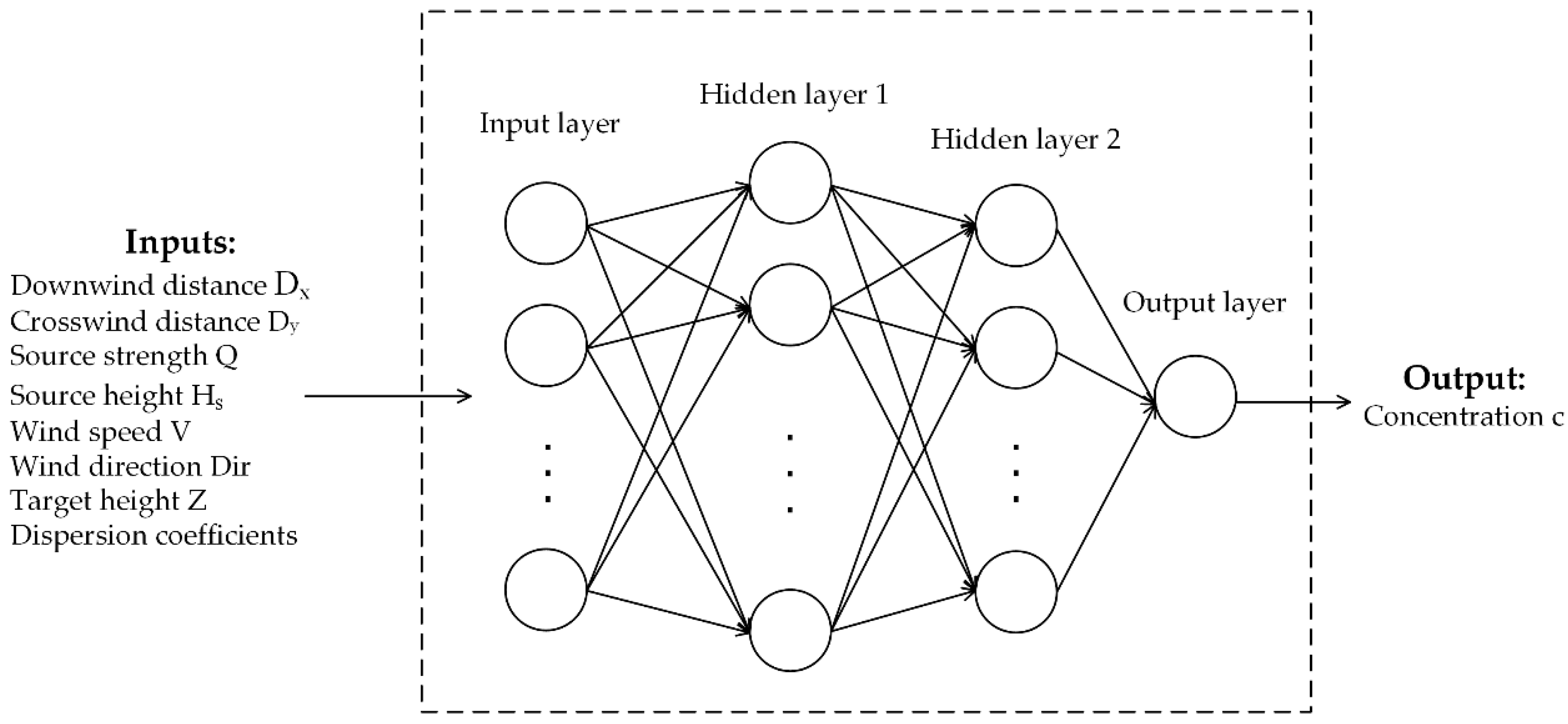
2.1. Structure of ANN

A desirable atmospheric dispersion prediction model with high accuracy and computational efficiency underlies the source estimation. Unfortunately, accurate atmospheric dispersion models, such as CFD and LS models, are time-consuming, while computationally efficient models, like the Gaussian model, are not accurate enough. To address this problem, ANN is applied to predict the concentration of interest points. As a machine learning algorithm, ANN is able to predict unknown complex relationships between its inputs and outputs with high accuracy. As for the computational efficiency, a trained ANN computes predictions rapidly. To predict the concentration of an interest point, the ANN needs some parameters in the hazardous gas dispersion as inputs. In gas dispersion, common original monitoring parameters are listed in Table 1. Selecting all the parameters is impractical, because numerous input parameters may increase the difficulty of training and slow down the convergence of the ANN. Therefore, only the main factors affecting the gas dispersion are selected as inputs of the ANN. In this paper, the selected parameters are D x ,   D y ,   Q ,   V ,   D i r ,   H s ,   Z , and dispersion coefficients a ,   b ,   c , and d . The four dispersion coefficients are significant parameters to determine the standard deviations in Gaussian models, shown in Equation (1):
{ σ y = a D x b σ z = c D x d
where σ y and σ z represent the standard deviations of Gaussian distributions in crosswind and vertical directions, respectively. D x is the downwind distance. The dispersion coefficients of a ,   b ,   c and d are derived from the atmospheric stability class [31] by Vogt’s scheme [32]. These selected parameters are essential factors for the atmospheric dispersion and are easy to measure. Moreover, they are inputs of many atmospheric dispersion models, like the Gaussian dispersion model. Therefore, these parameters are selected as the inputs of the ANN for dispersion prediction. In addition, it is worth mentioning that some researchers have taken integrated parameters like the Gaussian parameter as all inputs [16], in order to get more accurate predictions. This selection of inputs may help the ANN to perform well on synthetic datasets (especially those generated by Gaussian models). However, it is difficult for this kind of ANN to accurately reproduce the field data like the Indianapolis dataset [33], because Gaussian models are inaccurate under the condition of complex terrain. In contrast, most inputs of our ANN are original monitoring parameters, although the four dispersion coefficients in our ANN are parameters related to Gaussian models. Therefore, our ANN with inputs of original parameters is expected to have a good generalization in the field case. The structure of our prediction ANN, with inputs of original monitoring parameters, is shown in Figure 1. To achieve higher prediction accuracy, two hidden layers are applied. The neuron numbers of hidden layers can be adjusted according to the performance of the ANN. With appropriate neuron numbers of hidden layers, the ANN can perform well on both accuracy and the convergence speed. As for the output layer, there is only one neuron outputting the concentration of the interest point. The ANN is trained by the MATLAB neural network toolbox here, and the algorithm and detailed process of ANN training are introduced in the Section 3.2.

2.2. Solution Algorithm

Optimization is widely used in source estimation. For example, PSO is an intelligent optimization method, which drives numerous particles by specific rules in order to find the optimal solution with high computational efficiency. However, the original PSO algorithm tends to fall into the local optimum easily, especially when the search space is complex (e.g., multi-peak function). In contrast, SA has a strong global searching capacity, but runs slowly. Therefore, a hybrid optimization algorithm of PSO and SA is applied in this paper, to overcome the problems brought by the original optimization algorithms. In addition, wind field parameters (i.e., wind direction and wind speed) are estimated by the hybrid algorithm as well, because they have an impact on the accuracy of source estimation.
The hybrid algorithm is operated as follows. First, positions of N particles are randomly initialed in the search space, as well as the particle velocities. Each particle’s position is described as a 5-dimensional vector ( Q , x , y , V , D i r ) that represents a candidate solution of release rate, the two-dimensional coordinates of source, wind speed and wind direction. The fitness of each particle for the source estimation is evaluated by an objective function, described in Equation (2).
f i t n e s s ( p ) exp { 1 2 σ e 2 f ( p ) C o 2 }
where f ( p ) = { C p 1 , C p 2 , , C p n } and   C O = { C O 1 , C O 2 , , C O n } . p is the particle describing a candidate solution. f ( p ) is a vector representing the prediction concentrations of the ANN dispersion model at n receptor points with input p .   C O is a vector representing the observed concentrations at n receptors. Each observation is described as the sum of model value C m i and the measurement error e i : C O i   =   C m i +   e i   ( i = 1 , 2 , , n ) . n is the number of receptors whose observations are larger than zero. The zero-measurements are all removed. σ e 2 is a constant. A larger fitness means smaller prediction error and namely, a more accurate solution. Then the best position of each particle so far ( p b i ) and the best position of all particles ( g b ) as well as their fitness ( p b f i t i and g b f i t ) are initialized: the initial value of the ith particle is set as p b i , and the best p b i is set as g b . After that, the velocities and positions of all particles are updated according to Equation (3).
{ v i ( t ) = w · v i ( t 1 ) + c 1 r 1 ( p b i p i ( t 1 ) ) + c 2 r 2 ( g b p i ( t 1 ) ) p i ( t ) = p i ( t 1 ) + v i ( t ) .
where v i ( t ) represents the velocity of the ith particle in iteration t . p b i is the best position of the ith particle, while g b is the best position of all particles so far. w is the inertia parameter describing the weight of v i ( t 1 ) in the v i ( t ) . c 1 and c 2 are parameters adjusting the velocities towards the p b i and g b . r 1 and r 2 are two random numbers. This equation means that each particle’s movement is determined by combining its current velocity and position, its best position in history p b i , and the global best position g b . After the update of particle’s position and velocity, the fitness of these new particles is calculated by Equation (2). Subsequently, the p b i and g b are updated by simulated annealing. In typical PSO, if a new p b i or g b with better fitness appears in current iteration, the former p b i and g b are updated to the new values. However, this rule may result in an early-maturing result. Hence, the simulated annealing is applied in the update, making it possible to accept a “worse” solution in order to jump out of the local optimum. According to the simulated annealing algorithm, if either p b i or g b in the current iteration is better than the former, they are updated like the typical PSO. However, if not, there is still a probability for them accepting the new “worse” values. The acceptance probability is calculated by Equation (4):
{ p r o b = exp ( ( f i t n e w f i t ) / T ) T : = α T
where the n e w f i t and f i t are the value of p b f i t or g b f i t in the current and last iterations, respectively. T represents the temperature in the simulated annealing algorithm, and decays by rate α . Obviously, a smaller difference between two values of fitness and higher temperature means a larger acceptance probability. In the early stage of the algorithm operation, the large value of T guarantees a good global searching ability. Then, with the decay of T , the acceptance probability reduces gradually, promoting the convergence of the algorithm. Therefore, the hybrid algorithm tends to perform well on both global searching and local searching. This algorithm is operated iteratively until it converges, and the final g b is recognized as the estimation result of the source terms and wind field parameters. The procedure of this hybrid algorithm is shown in Algorithm 1.
Algorithm 1. Hybrid algorithm of PSO and SA
  • Initialize N particles with random positions and velocities in 5-demensional search space.
  • Initialize the p b i and g b as well as their fitness p b f i t i and g b f i t by Equation (2).
  • Loop
  • Update the velocities and positions of particles according to Equation (3).
  • For each particle, evaluate its fitness by Equation (2).
  • Compare each particle’s new fitness with its p b f i t i . If the new value of fitness is better than p b f i t i , set p b f i t i equal to the new value, and p b i equal to the new position. If new fitness is worse than p b f i t i , accept the new position as p b i with the acceptance probability calculated by Equation (4).
  • Compare p b f i t i with g b f i t . If p b f i t i is better than g b f i t , set g b f i t equal to p b f i t i , and g b equal to p b i . If p b f i t i is worse, accept p b i as g b with the acceptance probability calculated by Equation (4).
  • If a terminal condition is met (a sufficiently good fitness or a maximum number of iterations), exit loop.
  • End loop

3. Numerical Case Study

In this section, the source estimation method of a hybrid SAPSO algorithm with an ANN prediction model is tested on the synthetic data generated by a commercial software PHAST. To illustrate the improvement brought by the proposed method, the SAPSO algorithm’s performance is compared with two other algorithms (i.e., PSO coupled with ANN and PSO coupled with Gaussian model). The performances of these methods are evaluated by the skill score. Further, the influence of receptor configuration and measurement noise is analyzed. The procedure of this numerical experiment is shown as follows:
  • Define a number of leak scenarios in PHAST, and extract training data and test data from these scenarios.
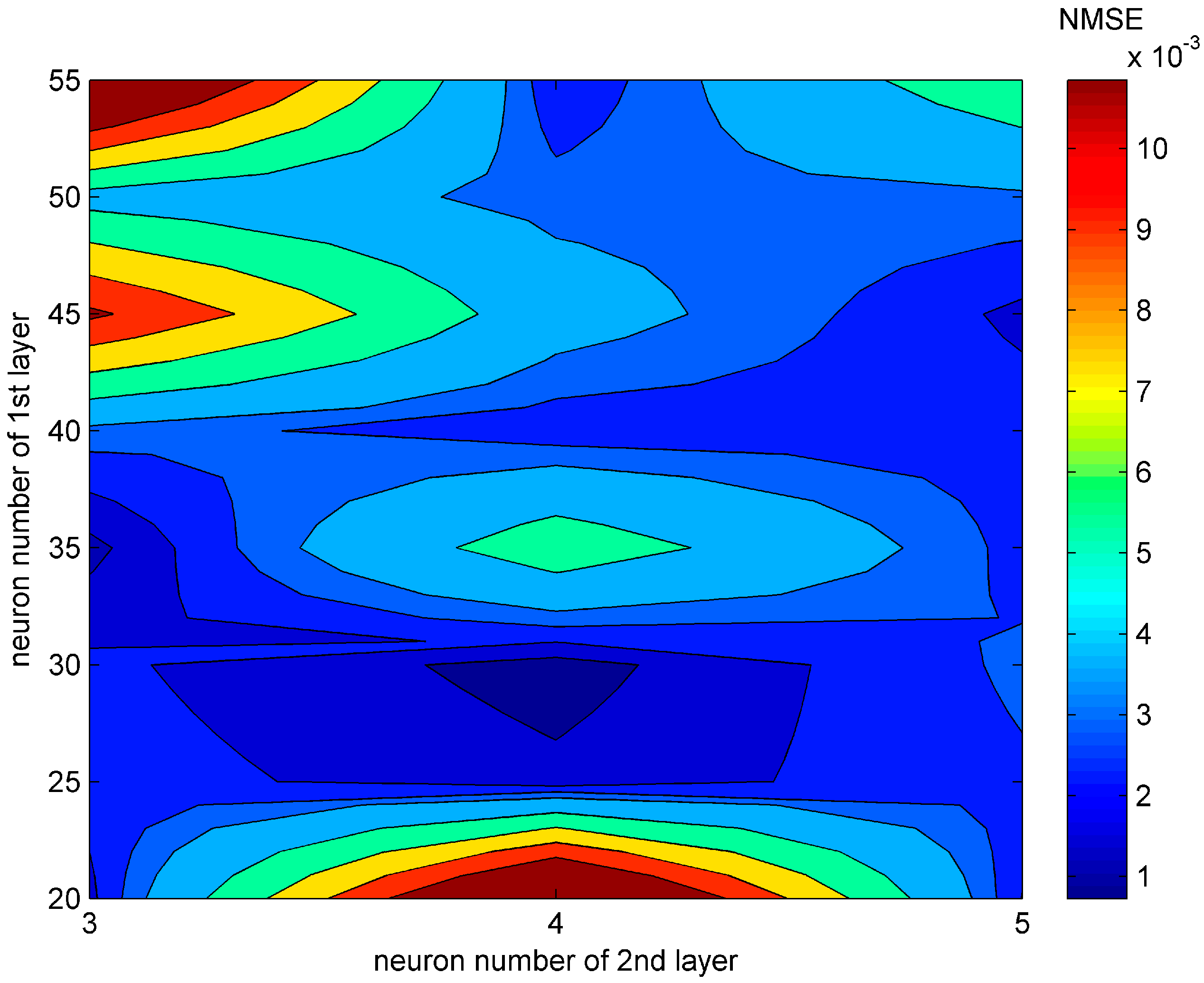
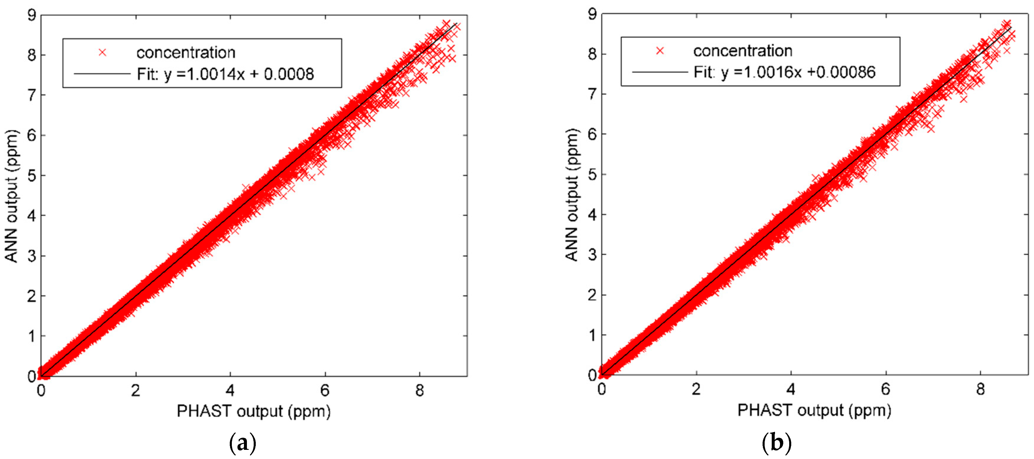
  • Train the ANN and adjust the neuron numbers of two hidden layers according to the performance. Test the performance of the trained ANN on the test data.
  • Define scenarios and generate receptor data for the source estimation.
  • Apply the proposed hybrid algorithm with an ANN to the source estimation and compare its performance with another two algorithms mentioned above.
  • Analyze the influence of receptor configuration and measurement noise on estimation result.

3.1. Synthetic Scenario

The numerical experiment is conducted in the synthetic scenarios generated by process hazard analysis software (PHAST). PHAST is a comprehensive process hazard analysis system of design and operation in the process industries [34]. In PHAST, a leak scenario can be defined by the leakage material type, source strength, release elevation, weather conditions (i.e., wind speed, wind direction, and atmospheric stability class), etc. In a leak scenario, the concentration data can be easily generated by the unified dispersion model (UDM) of PHAST. The UDM is for two-phase jet, heavy, and passive dispersion, including droplet rainout and pool spreading or evaporation [35]. It can model a wide range of scenarios, including the leak scenario in this paper. In this numerical experiment, the leakage material is chlorine (Cl2) and the leakage elevation is 45 m. Figure 2 shows a typical leakage scenario in the numerical experiment. It can be seen that there is an emission source located at (0 m, 0 m) with some receptors placed uniformly. The wind direction in this scenario is 135°. Based on the scenario in PHAST, the measured concentration data at receptors can be easily generated.
To generate enough training and test data for ANN, these scenario parameters are varied and combined to produce different scenarios, listed in Table 2. There are more than 1000 scenarios generated for ANN’s training and testing, covering the most common scenarios. Similar to the typical scenario in Figure 2, the source in these scenarios is located at (0 m, 0 m) with a height of 45 m. The source height in the synthetic data generation is fixed, and is not estimated by the source estimation algorithm. This setting of a fixed source height is based on the field case of the Shanghai chemical industry park that we focus on. In this chemical industry park, most emission sources have an elevation of 40–50 m. Therefore, we used the fixed source height of 45 m to simplify the calculation of ANN prediction and source estimation. The source location in the synthetic data generation is also fixed, because under the identical meteorological conditions and flat terrain condition, the source can generate the same concentration distribution (plume) at its downwind direction, regardless of the source location. Receptors are placed uniformly on the 1000 × 1000 m2 area with an interval of 50 m, and this receptor configuration is expressed as 21 × 21. All receptors are considered to be placed at ground. Based on the scenario parameters, corresponding leak scenarios are defined in PHAST. In all leak scenarios, sources release Cl2 continuously from 0 to 1000 s, and we only focus on the concentration data of the stable plume within the 1000 × 1000 m2 area. PHAST takes little terrain influence into consideration, so the terrain condition of this area is ideal and flat. Then, the receptor data of different scenarios, with no noise, is generated by the UDM in PHAST. The synthetic data of a scenario includes:
  • A set of downwind and crosswind distance of the target points from the release point: ( x 1 ,   x 2 ,   ,   x n ) and ( y 1 ,   y 2 ,   ,   y n ) , where n is the number of receptors;
  • The gas concentration at targets points (i.e., receptor data): ( c 1 ,   c 2 ,   ,   c n ) ;
  • The wind direction ( D i r ), speed ( V ), and atmospheric stability class ( S T A );
  • The source location ( S x ,   S y ) and strength ( Q ).
The parameters mentioned in Section 2.1 are derived from the scenario parameters and used as inputs of ANN, while the receptor data with no noise is the output of ANN (target). In addition, because the observed concentrations of many receptors are zero (e.g., receptors not in the downwind direction), these meaningless zero measurements could make ANN performance artificially excellent. To evaluate the prediction result fairly and reasonably, 70% of these zero samples are removed before the training process of ANN. The remaining data has 60,327 samples.
As for the source estimation, two test scenarios were defined, shown in the Table 3. It is worth mentioning that the two scenarios in this table were defined to test the algorithm performance with different source locations and some parameters close to the extreme range values (e.g., 180° wind direction and 2 m·s−1 wind speed). For each scenario, four receptor number configurations (6 × 6, 11 × 11, 21 × 21, and 51 × 51) were used. The receptor intervals of these configurations are 200 m, 100 m, 50 m, 20 m, respectively.

3.2. Configurations of the Artificial Neural Network and Optimization Algorithms

According to the network structure in Section 2.1, the corresponding ANN was constructed and trained. The data generated by PHAST (60,327 samples) was firstly mixed, and then randomly divided into the training set (50%, 30,163 samples), validation set (25%, 15,082 samples), and test set (25%, 15,082 samples). As for the network type, the BP network was suitable for a function-fitting problem like the dispersion prediction in this paper. This type of network has been used in dispersion prediction by many researchers [14,15]. Therefore, the BP network as applied here. The activation function of the neuron in the BP network is a tanh function. Compared with a sigmoid function, the tanh function tends to have a better performance with convergence speed and solution accuracy [36]. To get more accurate prediction results, the neuron numbers of two hidden layers were determined by calculating the normalized mean squared error (NMSE), shown in the Figure 3. By plotting the NMSE of different combinations of neuron numbers, we finally found that the ANN could obtain the lowest NMSE (0.0011) when the two hidden layers had 30 and 4 neurons, respectively. Afterwards, the training process was conducted by the MATLAB neural network toolbox. The training algorithm of the ANN is Levenberg–Marquardt, whose maximum number of epochs is 400 (if early stopping is not triggered). If accuracy on validation set showed no improvement after more than 6 epochs, the early stopping would be triggered.
In terms of the configuration of optimization algorithm, the PSO parameters c 1 , c 2 were both set to 2.0, and the inertia parameter w was set to 0.7. This selection of values is a common setting of the parameters c 1 , c 2 and w . This selection can give c 1 × r 1 or c 2 × r 2 a mean of 1.0, because the random values r 1 and r 2 follow the uniform distribution of [0, 1]. Therefore, the particle has an appropriate velocity and tends to get the target easily, which contributes to the convergence of the algorithm [23]. Similarly, the w of 0.7 also accelerates the convergence of the algorithm. The search range of each estimated parameter is displayed in Table 4. One hundred particles were randomly placed in the five-dimensional search space in both PSO and SAPSO, and the particle velocity in each dimension was randomly initialed and restricted within 10% of the search range in the corresponding dimension. With respect to the parameters of simulated annealing, the initial value of temperature T was 2000, while the decay rate α was 0.7. The values of T and α were adjusted by the algorithm performance on source estimation. Current values were selected from the intervals of [100, 10,000] and [0.5, 0.9], to balance the local searching with global searching. All source estimation algorithms mentioned were operated 50 times.

3.3. Skill Score

In this numerical case study, the skill score was constructed to evaluate the performances of different source estimation methods. The skill score combines individual component equations, each of which can quantify the accuracy of each parameter estimated by the algorithm. Similar to the Long [29], the component equations are:
S q =   | Q a c t Q e s t | Q a c t
S x = max ( (   x a c t x e s t ) ( x a c t x m i n )   , (   x e s t x a c t ) (   x m a x x a c t ) )
S v =   | V a c t V e s t | V a c t
S d i r = m i n ( | D i r a c t D i r e s t | ,   360 | D i r a c t D i r e s t | ) / 90
where the “act” and “est” designations refer to the actual values and estimated values, respectively. The “min” and “max” designations represent the minimum and maximum values in search space shown in Table 4. The skill scores of S q and S v represent the relative errors of source strength and wind speed, respectively. The S x and S y describe the location error with the search range. If x e s t or y e s t reaches the maximum or minimum of the search range, the corresponding skill score is 1.0. The design of S d i r is to deal with some special values (e.g., | D i r a c t D i r e s t | > 180°). Further, these skill scores are set to 1.0 if they exceed 1.0. Therefore, their ranges are limited to [0, 1.0]. Based on these equations, the total skill score for the estimation of five parameters can be described as:
S k i l l S c o r e = ( w 1 S q + w 2 S x + w 3 S y + w 4 S v + w 5 S d i r ) / 5
where w i ,   i = 1 , 2 , 3 , 4 , 5 are the weights of the five skill scores mentioned above. These weights can be adjusted according to the estimation result for the desired total skill score. Here, they are 2.0, 5.0, 5.0, 2.0, and 1.0, respectively. These weights are set to reflect the importance of the five parameters and differences of algorithm performances in various scenarios. Among the five parameters, the source location is usually the most important, so the w 2 and w 3 are both set to large values (5.0). In addition, according to the estimation results, the wind speed V and source strength Q are relatively difficult to estimate. Therefore, w 1 and w 4 are set to be 2.0, to increase these two skill scores and to reflect the differences of algorithm performances clearly. It is obvious that the most desirable skill score is zero.

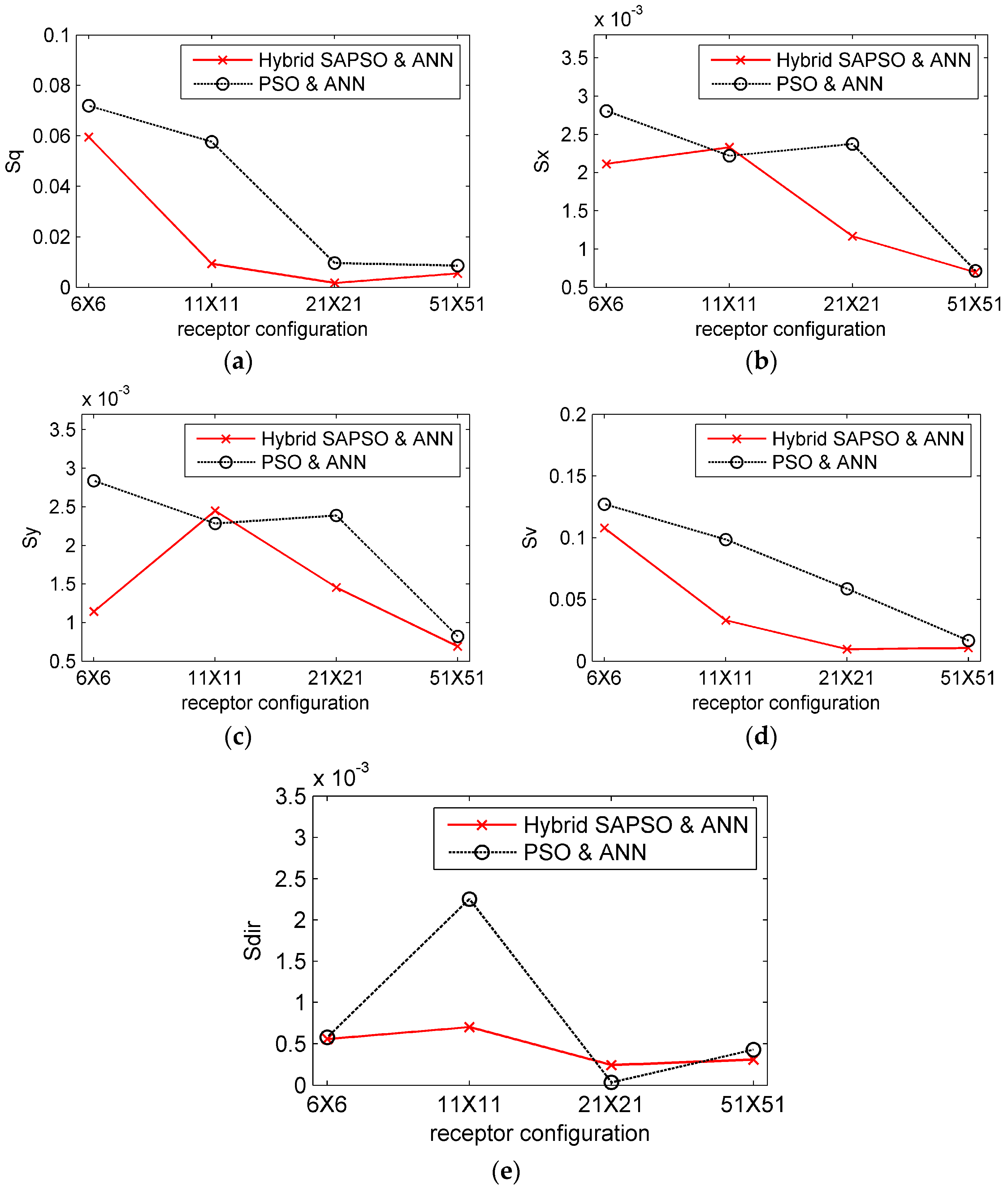
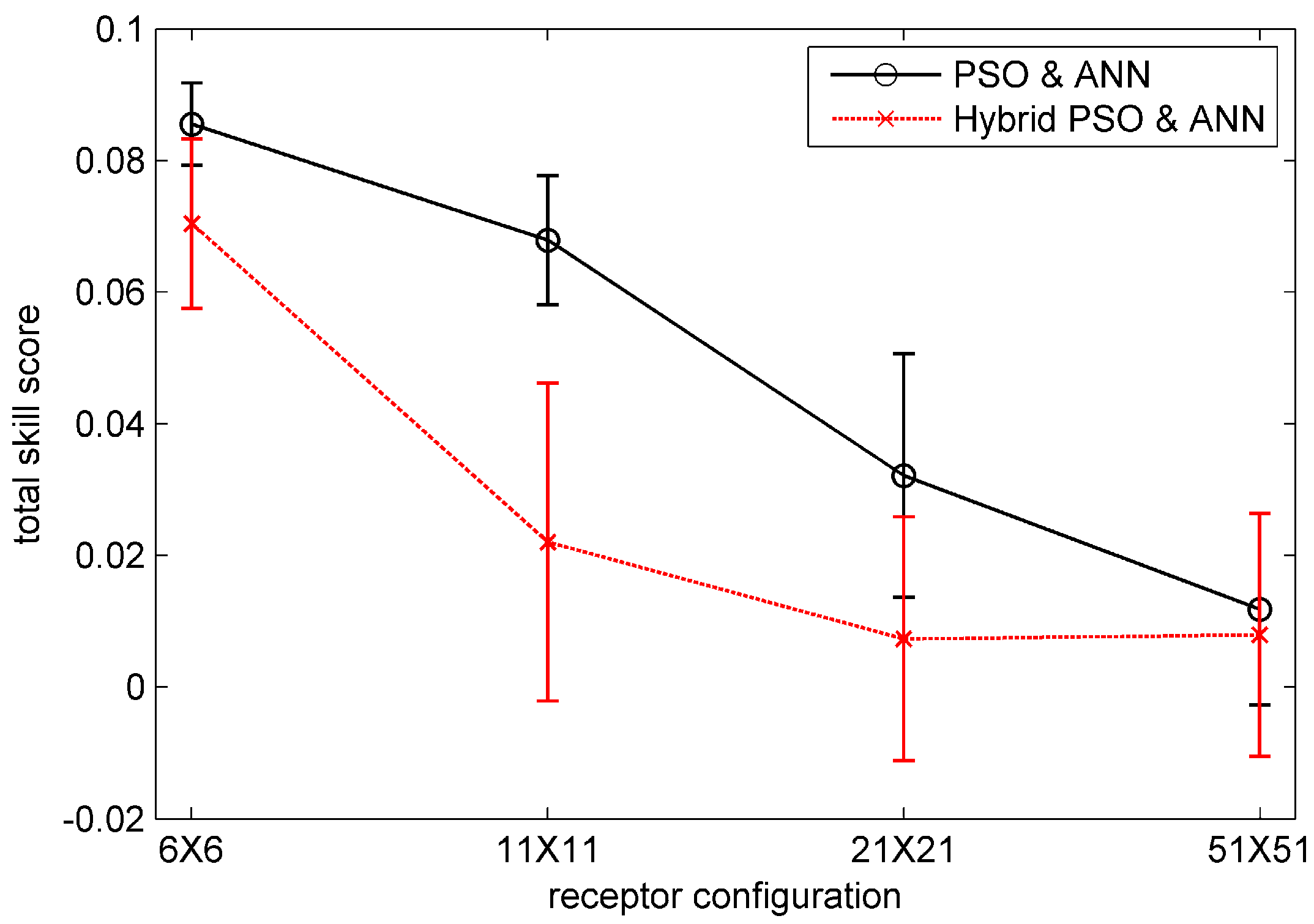
3.4. Results and Analysis

The ANN prediction concentrations on training data and test data are shown in Figure 4. As shown in Figure 4, the prediction concentrations of ANN on the training and test set were both quite close to the pre-determined concentrations, with the fitting line close to “y = x”. To further evaluate the ANN performance on the test data, the indicators of the correlation coefficient (R2), normalized mean squared error (NMSE), and fractional bias (FB) were used [37]. The R2 of results on test data was high (0.9986), and the NMSE and FB were both quite close to zero (−0.0016 and 0.0011, respectively). These indicators all illustrate the excellent performance of ANN on the test data. In addition, the results on the test set also demonstrate that, when trained by training data covering most scenarios, the ANN has a good generalization. Therefore, the ANN is a good way of modeling and predicting the hazardous gas dispersion in the numerical experiment.
Applying ANN in the hybrid SAPSO and PSO algorithms, we can get the average estimation results of 50 runs on the two test scenarios, shown in Table 5 and Table 6. In addition, the individual skill scores of five estimated parameters in Scenario 1 are shown in Figure 5. In these tables, the result with total skill score lower than 0.05 is considered to be accurate. Table 5 shows that the two algorithms were both able to estimate each parameter accurately with 21 × 21 receptors or more, shown by small total skill scores (less than 0.05) and the individual skill scores (all less than 0.05) in Figure 5. With fewer receptors (11 × 11), the SAPSO and ANN still maintained high accuracy (0.0220 total skill score), while the estimation accuracy of PSO and ANN decreased (0.0679 total skill score). The difference is mainly from the wind speed; the wind speed estimated by PSO and ANN was 3.6059 (with error −0.3941), which is approximately 10% lower than the actual value. In contrast, the result of SAPSO and ANN was 3.8678, with only a 3.3% error (−0.1322). Further, when the receptor number decreases to 6 × 6, the performances of the two algorithms were both unsatisfactory, indicated by the total skill scores (both larger than 0.05) in Table 5. The similar results can be also seen from the skill scores in Figure 5. Compared with PSO and ANN, the hybrid algorithm of SAPSO and ANN performed better on estimation with all receptor configurations, especially on the source strength ( Q ) and wind speed ( V ), seen from the Figure 5a,d. This comparison implies that the simulated annealing algorithm used in the PSO helps to jump out of the local optimum, and improves the results consequently. In addition, it should be noted that the improvement of the hybrid SAPSO and ANN is more significant when the receptor configuration is 11 × 11 or 21 × 21 than with the other two receptor configurations. Similar conclusions can be drawn from Table 6—that two algorithms get accurate estimation results with more than 11 × 11 receptors, and that the hybrid algorithm has a better performance than PSO algorithm. In addition, Table 6 also shows the excellent performances of two algorithms in a different scenario with some extreme parameters (e.g., 180° wind direction and 2 m/s wind speed). Moreover, the accurate estimation of the source location in Table 6 illustrates that the proposed algorithm is feasible and accurate with different source location (300, −300), even if the training data of the ANN is generated from the fixed location source (0, 0).
The results in Table 5 also show the differences in estimation accuracy of different parameters. As seen from the Figure 5, with low skill scores (lower than 0.3%) for all receptor configurations, the wind direction ( D i r ) and source location (x,y) are estimated accurately by both algorithms. In contrast, the skill scores of source strength ( Q ) and wind speed ( V ) are larger, as well as the difference of results between the two algorithms. This comparison may reflect that the atmospheric dispersion is more sensitive to the wind direction ( D i r ) and source location ( x , y ). Therefore, these parameters are estimated more easily. As for the computational efficiency, the computing time values of the two algorithms demonstrate their acceptable efficiency. To further evaluate the performances of the two algorithms, their mean objective function values ( g b f i t in each iteration, Equation (2)) of 50 runs during the experiment of Scenario 1 are shown in Figure 6. It can be seen from this figure that during the calculation process, the objective function values of the two algorithms both rise at first, and later stabilize. Compared with the PSO algorithm, the hybrid algorithm has lower values of objective function in the early stage of the calculation. However, the hybrid algorithm gets a higher objective function in the later period, and its final value is closer to the perfect value (1.0). The possible reason for this result is the simulated annealing used in PSO. The possible acceptance of worse p b f i t i and g b f i t results in the lower objective function of the hybrid algorithm in the early stage. Meanwhile, the simulated annealing improves the global searching ability, so the final objective function value of the hybrid algorithm is better than the PSO algorithm.
In order to make further comparison of the two algorithms, the average skill scores with standard deviations in Scenario 1 are shown in Figure 7. Obviously, the skill scores of the two algorithms decreased when the receptor number increased, indicating that the estimation becomes easier with more receptors. For most of receptor configurations, the solutions of PSO and ANN were improved by the hybrid algorithm, which is consistent with Table 5. However, the hybrid algorithm has a larger standard deviation. This may be because the acceptance of worse fitness in simulated annealing increases the uncertainty of estimation solutions. As for the source estimation algorithm of the PSO and Gaussian model, it was operated 50 times with 51 × 51 receptors. The average estimation results of this algorithm in Scenario 1 were 37.5825 g·s−1, 53.5409 m, 74.6308 m, 2.5390 m·s−1, and 145.3857°, with 0.51 s computing time. Although the PSO and Gaussian model method has faster computing than aforementioned two algorithms, its estimation results are far from satisfactory, due to the poor accuracy of the simple Gaussian model. Therefore, the proposed method of a hybrid SAPSO and ANN model is able to effectively improve the estimation accuracy of conventional optimization methods (i.e., PSO and ANN or the PSO and Gaussian model) in the numerical case.

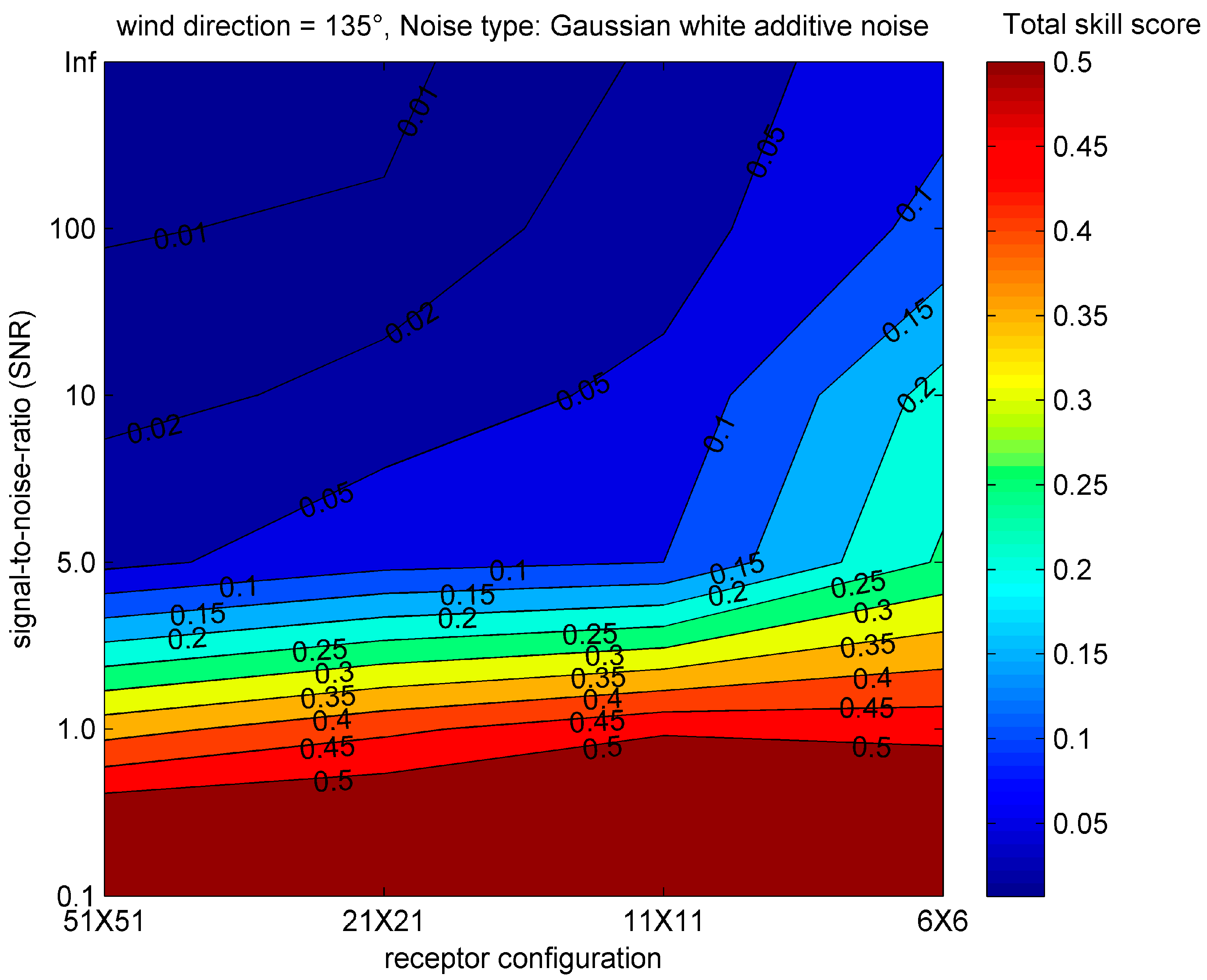
3.5. The Influence of Noisy Observation

In the aforementioned experiment, the receptor data is generated with no measurement noise. However, measurement noise is inevitable in practice, and has a significant impact on the source estimation. Hence, the hybrid algorithm is performed with receptor data perturbed by Gaussian white additive noise here, in order to observe the influence of measurement noise. The noises have six different signal-to-noise ratios (SNRs): 0.1, 1.0, 5.0, 10, 100 and infinity (no noise). The SNR here is defined by dividing the actual concentration (signal) by measurement noise, which is somewhat different from the definition of SNR in electronics. An SNR above 1.0 indicates less noise than signal, while an SNR below 1.0 indicates more noise than signal. Furthermore, each of these runs is performed repeatedly with each of four receptor configurations (6 × 6, 11 × 11, 21 × 21, and 51 × 51) to evaluate the sensitivity of estimation results to receptor configuration and noise. The wind direction in these runs is 135°.
Figure 8 shows the contour plot of median total skill scores across 20 runs as a function of receptor configurations and SNRs in Scenario 1. The median skill score is considered here instead of the mean, because the median is less sensitive to outliers. An estimation result with a skill score lower than 0.05 is considered acceptable. The influence of receptor configuration and SNR on the skill score can be illustrated clearly by this figure. Obviously, the SNR influences the result greatly with each of receptor configurations. In most cases, with an SNR larger than 10, the source terms and wind field parameters can be estimated accurately. However, the performance of the hybrid algorithm deteriorates sharply with an SNR lower than 5.0, indicated by the dense contours between SNR = 5.0 and SNR = 1.0. If the SNR is lower than 1.0, the hybrid algorithm is unable to compute the solution to any reasonable degree of accuracy (with a skill score larger than 0.4). With this much noise, the actual plume can no longer be detected precisely from the receptor data, so the hybrid algorithm is of no use. Furthermore, runs with more receptors are less sensitive to noise than runs with fewer receptors. As for the impact of receptor number, the skill score is appreciably affected by receptor configuration only if the SNR is relatively high (5.0–100), as seen from the contours of 0.2, 0.1, 0.05, 0.02 and 0.01.

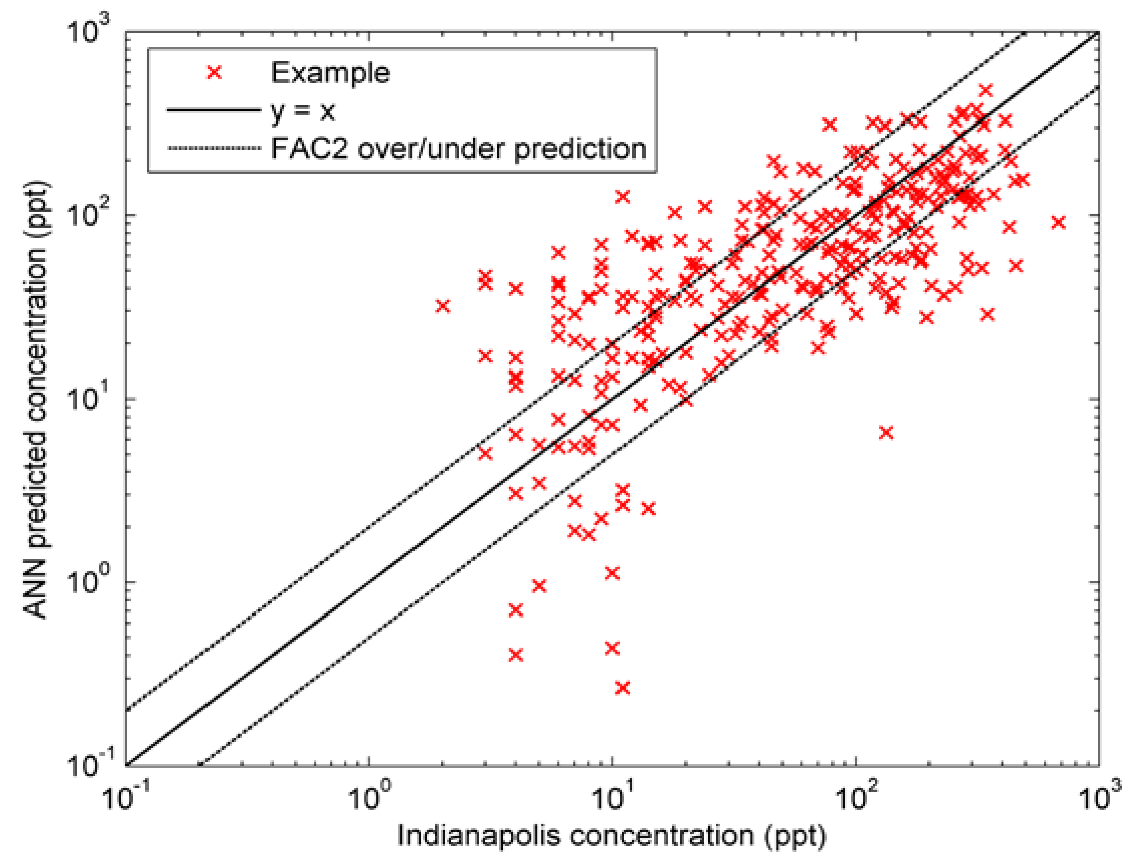
4. Indianapolis Field Study

4.1. Introduction of the Indianapolis Tracer Experiment

In order to verify the effectiveness of proposed method in the field, the proposed method of SAPSO coupled with ANN was tested on the Indianapolis tracer dataset [33]. This tracer experiment was conducted in Indianapolis, Indiana, U.S., from 16 September to 11 October 1985. In this experiment, the S F 6 tracer was released from an 83.8 m stack (with diameter 4.72 m) at the Perry K power plant in Indianapolis. The geographic coordinates of this stack are UTM-N 4401.59 km (39.8° E latitude) and UTM-E 571.40 km (86.2° E longitude). The 83.8 m stack at the Perry K plant was located in a typical urban area, with many buildings within one or two kilometers of the stack [38]. Therefore, the terrain condition of this experiment was quite complex. As for the experimental data, 170 h of tracer concentration data is available, as well as the meteorological data representing all atmospheric stability classes and most wind direction and speed ranges. The tracer concentrations were observed by a network of about 160 ground-level monitors in semi-circular arcs, at distances ranging from 0.25 to 12.0 km from the stack. Therefore, the range of the monitoring distance was about 12 km. The unit of the tracer data is ppt (one millionth of ppm). The meteorological data was collected by various sensors [38]. Data were taken in 8 or 9 h blocks each day. There are a total of 19 such blocks in the Indianapolis dataset, representing the data of different days.

4.2. Configurations of the Artificial Neural Network and the Solution Algorithm

To evaluate the ANN’s performance reasonably, the zero measurements were removed, like in the numerical experiment. The tracer and meteorological data from 18 September to 11 October was used for training and validation (70% and 30% respectively, 4859 samples in total) while the data of 17 September were used for testing (311 samples). It is worth mentioning that there were different monitoring values for wind speed and direction at the same time in the Indianapolis dataset. They were measured by four meteorological stations. Therefore, the ANN here had 21 inputs (i.e., four different wind speeds V , directions D i r , downwind distances D x , crosswind distances D y , four dispersion coefficients a , b , c , and d , and source strength Q ). The neuron numbers of two layers were 60 and 7, respectively, due to the increased number of inputs (compared with the numerical experiment). Other configurations of the ANN are the same as the numerical experiment. Only the source terms were estimated in this experiment, because it was difficult to estimate several wind speeds and directions with this dataset, and the wind field is considered known here. The data from 11 a.m. on 17 September was used as test data for source estimation. Each algorithm used 30 particles and was performed 50 times, because the number of estimated parameters was only three. The selection of c 1 ,   c 2 ,   w ,   T and α was the same as the numerical experiment.

4.3. Results and Analysis

Figure 9 demonstrates the comparison between the Indianapolis measurements and the ANN prediction results. Obviously, most examples are distributed around the perfect fitting line: y = x. To reasonably evaluate the performance of the ANN, all zero measurements were removed when plotting the figure. To further evaluate the performance of the ANN prediction model, the R2 coefficient, factor of two (FAC2), FB, and NMSE were applied here. The R2 of the all predicted results and the measurements was 0.5655, illustrating that the predicted concentrations were close to the measurements. The FAC2 of the prediction results without zero measurements was 0.5305, indicating that the ANN prediction model has an acceptable performance, according to the criteria FAC2 > 0.5 [39]. The FAC2 over and under prediction lines (i.e., y = 2x and y = x/2, respectively) are also shown in the figure. Furthermore, the FB of the result was 0.2005 and the NMSE was 0.6054, which are close to zero and prove the acceptable performance. To compare the ANN output reliably, the receptor distribution in the domain at 11:00 a.m. on 17 September is shown in the Figure 10. In this figure, the values of the receptor data is roughly described by the size of the black filled circle in the figure; the larger circle represents the higher observed concentration. This figure combines the receptor distribution and the observed data, giving a direct visualization of the dispersion scenario.
As for the source estimation, the average estimation results listed in Table 7 illustrate that the two algorithms are both able to obtain acceptable results. The source location errors of the two algorithms were 94.27 m and 93.35 m, and the relative errors to the monitoring area length (12 km) were 0.786% and 0.778%, respectively. The results illustrate that the proposed source estimation methods are feasible in practice. However, the similar performances of the two algorithms indicates that the improvement of the hybrid algorithm is less significant than in the numerical experiment. This may result from the accuracy of the ANN prediction model. The ANN in this field case study is not as accurate as that in the numerical experiment. Therefore, the estimation accuracy is mainly affected by the accuracy of ANN instead of the source estimation algorithm. In addition, it can be seen from this table that the source strength, which is difficult to estimate in a numerical experiment, is accurately estimated by the two algorithms. The difference results from the narrow range of source strength in the Indianapolis dataset.

5. Discussion

In the numerical experiment, the hybrid SAPSO algorithm and ANN indeed improves the estimation accuracy of the PSO and ANN. It is worthwhile to note that the improvement brought by the hybrid SAPSO is more significant with 11 × 11 and 21 × 21 receptors than with the other two receptor configurations in both test scenarios. With 51 × 51 receptors, the performances of both algorithms are satisfying, with total skill scores lower than 0.015, and the difference of their skill scores is small. These results indicate that using a large number of receptors may help to make up for the accuracy of the source estimation algorithm. In addition, the large total skill scores (larger than 0.05) of both algorithms with 6 × 6 receptors imply that having enough receptors is indispensable for source estimation. The lack of receptors may lead to inaccurate source estimation, even if the algorithm is excellent. These findings provide some guidance for the configuration of receptors and the selection of a source estimation algorithm in emergency management. Besides, although the hybrid algorithm improves the PSO, it brings greater standard deviation, because of the possible acceptance of worse fitness in simulated annealing, as indicated by Figure 7. In order to reduce the uncertainty of estimation results, the parameters of temperature T and decay rate α should be further optimized to balance the global searching with local searching. Different decay modes, such as T ( t ) = c / log ( 1 + t ) , can be applied [40]. Operating the algorithm many times may help as well. In addition, the estimation results of Scenario 2 illustrate that the proposed algorithm is feasible and accurate in a different scenario and with a different source location (300, −300) and some extreme parameters, even if the ANN used in the algorithm is trained by the synthetic data generated from a fixed-location source (0, 0).
As for the field case study, the improvement brought by simulated annealing in the Indianapolis case study is less significant than in the numerical experiment. The possible reason may be the accuracy of ANN prediction model. Because of the complexity of the Indianapolis field dataset, the ANN cannot predict the gas dispersion as accurately as the ANN in the numerical experiment. Therefore, affected by the ANN prediction model, the estimation accuracy is not improved significantly by the hybrid algorithm. To deal with this problem, more accurate ANNs like the deep neural network will be applied to the dispersion prediction in the future work.
However, the method proposed in this paper also has some problems. The main problem is the PHAST software used in the numerical case study. Since it takes few terrain conditions into consideration, the UDM in PHAST is still not accurate enough to describe the actual dispersion, making the synthetic data easy to predict. Besides, the wind field in a scenario of PHAST is stable and identical in the 1000 × 1000 m2 area, while the actual wind field is unevenly distributed. The actual uneven wind field can make a significant difference to hazardous gas dispersion in air. Therefore, although the proposed ANN and source estimation method has an excellent performance with PHAST data, it may be not feasible in the field. To deal with the problem, more accurate commercial software should be applied, such as the AERMOD [41] and CALPUFF [42], to produce more realistic dispersion data. Based on these sophisticated models, the constructed ANN and source estimation method can be more convincing.

6. Conclusions

This paper proposed a novel method for estimating hazardous source terms and wind field parameters using ANN, PSO, and SA. The ANN is applied in order to model and predict the atmospheric dispersion of hazardous gas accurately and efficiently, while the hybrid algorithm of SAPSO is used to improve the global searching of the original PSO. A numerical case study is implemented based on PHAST, to test the performance of the proposed method, and the Indianapolis field study proves that this method is feasible in practice. Results illustrate that the ANN, with both accuracy and efficiency, provides a more desirable forward dispersion model for the source estimation algorithm than the Gaussian model. In addition, the hybrid algorithm of SAPSO improves the estimation accuracy of the original PSO algorithm, especially in the numerical case study. In conclusion, the proposed method is able to estimate the hazardous source and wind field with both accuracy and efficiency. Therefore, this method will provide strong support to the emergency management of hazardous leak accidents in the future. Future work includes the application of the sophisticated software on the dispersion data generation, application of the deep neural network on the gas dispersion modeling, and the field experiment of the proposed method (e.g., in the Shanghai chemical industry park).

Acknowledgments

This study is supported by National Key Research and Development (R&D) Plan under Grant No. 2017YFC0803300 and the National Natural Science Foundation of China under Grant Nos. 71673292, 61503402 and National Social Science Foundation of China under Grant No. 17CGL047 and Guangdong Key Laboratory for Big Data Analysis and Simulation of Public Opinion.

Author Contributions

Rongxiao Wang and Sihang Qiu conceived and designed the experiments; Rongxiao Wang performed the experiments under the guidance of Bin Chen; Zhengqiu Zhu analyzed the data; Xiaogang Qiu, Yiping Wang and Liang Ma gave important suggestions for data analysis; Rongxiao Wang wrote the paper.

Conflicts of Interest

The authors declare no conflict of interest.

References

  1. Zhu, Z.; Chen, B.; Reniers, G.; Zhang, L.; Qiu, S.; Qiu, X. Playing chemical plant environmental protection games with historical monitoring data. Int. J. Environ. Res. Public Health 2017, 14, 1155. [Google Scholar] [CrossRef] [PubMed]
  2. Chen, B.; Zhang, L.; Guo, G.; Qiu, X. KD-ACP: A software framework for social computing in emergency management. Math. Probl. Eng. 2015, 2015, 27. [Google Scholar] [CrossRef]
  3. Hutchinson, M.; Oh, H.; Chen, W.-H. A review of source term estimation methods for atmospheric dispersion events using static or mobile sensors. Inf. Fusion 2017, 36, 130–148. [Google Scholar] [CrossRef]
  4. Wang, R.; Chen, B.; Qiu, S.; Zhu, Z.; Qiu, X. Data assimilation in air contaminant dispersion using a particle filter and expectation-maximization algorithm. Atmosphere 2017, 8, 170. [Google Scholar] [CrossRef]
  5. Briggs, G.A. Diffusion Estimation for Small Emissions. Preliminary Report; Atmospheric Turbulence and Diffusion Laboratory; NOAA: Silver Spring, MD, USA, 1973.
  6. Hanna, S.R.; Briggs, G.A.; Hosker, R.P.; Smith, J.S.; United States. Department of Energy. Office of Energy Research; United States. Department of Energy. Office of Health and Environmental Research. Handbook on Atmospheric Diffusion; U.S. Department of Energy: Washington, DC, USA, 1982; p. 102.
  7. Flesch, T.K.; Wilson, J.D.; Yee, E. Backward-time lagrangian stochastic dipsersion models and their application to estimate gaseous emissions. J. Appl. Meteorol. 1995, 34, 1320–1332. [Google Scholar] [CrossRef]
  8. Wilson, J.D.; Sawford, B.L. Review of lagrangian stochastic models for trajectories in the turbulent atmosphere. Bound. Layer Meteorol. 1996, 78, 191–210. [Google Scholar] [CrossRef]
  9. Pontiggia, M.; Derudi, M.; Busini, V.; Rota, R. Hazardous gas dispersion: A CFD model accounting for atmospheric stability classes. J. Hazard. Mater. 2009, 171, 739–747. [Google Scholar] [CrossRef] [PubMed]
  10. Xing, J.; Liu, Z.; Huang, P.; Feng, C.; Zhou, Y.; Zhang, D.; Wang, F. Experimental and numerical study of the dispersion of carbon dioxide plume. J. Hazard. Mater. 2013, 256–257, 40–48. [Google Scholar] [CrossRef] [PubMed]
  11. Bieringer, P.E.; Rodriguez, L.M.; Vandenberghe, F.; Hurst, J.G.; Bieberbach, G.; Sykes, I.; Hannan, J.R.; Zaragoza, J.; Fry, R.N. Automated source term and wind parameter estimation for atmospheric transport and dispersion applications. Atmos. Environ. 2015, 122, 206–219. [Google Scholar] [CrossRef]
  12. Pelliccioni, A.; Tirabassi, T. Air dispersion model and neural network: A new perspective for integrated models in the simulation of complex situations. Environ. Model. Softw. 2006, 21, 539–546. [Google Scholar] [CrossRef]
  13. Podnar, D.; Koračin, D.; Panorska, A. Application of artificial neural networks to modeling the transport and dispersion of tracers in complex terrain. Atmos. Environ. 2002, 36, 561–570. [Google Scholar] [CrossRef]
  14. Boznar, M.; Lesjak, M.; Mlakar, P. A neural network-based method for short-term predictions of ambient SO2 concentrations in highly polluted industrial areas of complex terrain. Atmos. Environ. Part B Urban Atmos. 1993, 27, 221–230. [Google Scholar] [CrossRef]
  15. Bing, W.; Bingzhen, C.; Jinsong, Z. The real-time estimation of hazardous gas dispersion by the integration of gas detectors, neural network and gas dispersion models. J. Hazard. Mater. 2015, 300, 433–442. [Google Scholar]
  16. Ma, D.; Zhang, Z. Contaminant dispersion prediction and source estimation with integrated gaussian-machine learning network model for point source emission in atmosphere. J. Hazard. Mater. 2016, 311, 237–245. [Google Scholar] [CrossRef] [PubMed]
  17. Qiu, S.; Chen, B.; Wang, R.; Zhu, Z.; Wang, Y.; Qiu, X. Estimating contaminant source in chemical industry park using UAV-based monitoring platform, artificial neural network and atmospheric dispersion simulation. RSC Adv. 2017, 7, 39726–39738. [Google Scholar] [CrossRef]
  18. Qiu, S.; Chen, B.; Wang, R.; Zhu, Z.; Wang, Y.; Qiu, X. Atmospheric dispersion prediction and source estimation of hazardous gas using artificial neural network, particle swarm optimization and expectation maximization. Atmos. Environ. 2018, 178, 158–163. [Google Scholar] [CrossRef]
  19. Johannesson, G.; Hanley, B.; Nitao, J. Dynamic Bayesian Models via Monte Carlo—An Introduction with Examples; Lawrence Livermore National Laboratory: Livermore, CA, USA, 2004. [Google Scholar]
  20. Keats, A.; Yee, E.; Lien, F.S. Bayesian inference for source determination with applications to a complex urban environment. Atmos. Environ. 2007, 41, 465–479. [Google Scholar] [CrossRef]
  21. Wawrzynczak, A.; Kopka, P.; Borysiewicz, M. Sequential monte carlo in bayesian assessment of contaminant source localization based on the sensors concentration measurements. In Parallel Processing and Applied Mathematics, Revised Selected Papers, Part II, Proceedings of the 10th International Conference, PPAM 2013, Warsaw, Poland, 8–11 September 2013; Wyrzykowski, R., Dongarra, J., Karczewski, K., Waśniewski, J., Eds.; Springer: Berlin/Heidelberg, Germany, 2014; pp. 407–417. [Google Scholar]
  22. Zheng, X.; Chen, Z. Back-calculation of the strength and location of hazardous materials releases using the pattern search method. J. Hazard. Mater. 2010, 183, 474–481. [Google Scholar] [CrossRef] [PubMed]
  23. Kennedy, J. Particle swarm optimization. In Proceedings of the 1995 IEEE International Conference on Neural Networks, Perth, Australia, 27 November–1 December 1995; pp. 1942–1948. [Google Scholar]
  24. Ma, D.; Deng, J.; Zhang, Z. Comparison and improvements of optimization methods for gas emission source identification. Atmos. Environ. 2013, 81, 188–198. [Google Scholar] [CrossRef]
  25. Qiu, S.; Chen, B.; Zhu, Z.; Wang, Y.; Qiu, X. Source term estimation using air concentration measurements during nuclear accident. J. Radioanal. Nucl. Ch. 2017, 311, 165–178. [Google Scholar] [CrossRef]
  26. Thomson, L.C.; Hirst, B.; Gibson, G.; Gillespie, S.; Jonathan, P.; Skeldon, K.D.; Padgett, M.J. An improved algorithm for locating a gas source using inverse methods. Atmos. Environ. 2007, 41, 1128–1134. [Google Scholar] [CrossRef]
  27. Allen, C.T.; Young, G.S.; Haupt, S.E. Improving pollutant source characterization by better estimating wind direction with a genetic algorithm. Atmos. Environ. 2007, 41, 2283–2289. [Google Scholar] [CrossRef]
  28. Allen, C.T.; Haupt, S.E.; Young, G.S. Source characterization with a genetic algorithm coupled dispersion backward model incorporating scipuff. J. Appl. Meteorol. Climatol. 2007, 46, 273–287. [Google Scholar] [CrossRef]
  29. Long, K.J.; Haupt, S.E.; Young, G.S. Assessing sensitivity of source term estimation. Atmos. Environ. 2010, 44, 1558–1567. [Google Scholar] [CrossRef]
  30. Haupt, S.E.; Young, G.S.; Allen, C.T. A genetic algorithm method to assimilate sensor data for a toxic contaminant release. J. Comput. 2007, 2, 85–93. [Google Scholar] [CrossRef]
  31. Carrascal, M.D.; Puigcerver, M.; Puig, P. Sensitivity of gaussian plume model to dispersion specifications. Theor. Appl. Climatol. 1993, 48, 147–157. [Google Scholar] [CrossRef]
  32. Vogt, K.J. Empirical investigations of the diffusion of waste air plumes in the atmosphere. Nucl. Technol. 1977, 34, 43–57. [Google Scholar] [CrossRef]
  33. Steven Hanna, J.C.; Olesen, H.R. Indianapolis Tracer Data and Meteorological Data; National Environmental Research Institute: Roskilde, Denmark, 2005. [Google Scholar]
  34. Phast. Available online: https://www.dnvgl.com/services/process-hazard-analysis-software-phast-1675 (accessed on 29 December 2017).
  35. Henk, W.M.; Witloxa, M.H.; Pitbladob, R. Validation of phast dispersion model as required for USA lng siting applications. Chem. Eng. Trans. 2013, 31, 49–54. [Google Scholar]
  36. Li, X. A comparison between information transfer function sigmoid and tanh on neural. J. Wuhan Univ. Technol. 2004, 28, 312–314. [Google Scholar]
  37. Lauret, P.; Heymes, F.; Aprin, L.; Johannet, A. Atmospheric dispersion modeling using artificial neural network based cellular automata. Environ. Model. Softw. 2016, 85, 56–69. [Google Scholar] [CrossRef]
  38. Chang, J.C.; Hanna, S.R. Air quality model performance evaluation. Meteorol. Atmos. Phys. 2004, 87, 167–196. [Google Scholar] [CrossRef]
  39. Hajek, B. Cooling schedules for optimal annealing. Math. Oper. Res. 1988, 13, 311–329. [Google Scholar] [CrossRef]
  40. Cimorelli, A.J.; Perry, S.G.; Lee, R.F.; Paine, R.J.; Venkatram, A.; Weil, J.C.; Wilson, R.B. Aermod Description of Model Formulation Version; EPA: Washington, DC, USA, 1998.
  41. Scire, J.S.; Strimaitis, D.G.; Yamartino, R. A User’s Guide for the Calpuff Dispersion Model; Earth Tech, Inc.: Somerset, PA, USA, 2000. [Google Scholar]
  42. TRC Environmental Consultants. Urban Power Plant Plume Studies; EPRI: Palo Alto, CA, USA, 1986. [Google Scholar]
Figure 1. The structure of the prediction artificial neural network (ANN), with inputs of original monitoring parameters.
Atmosphere 09 00119 g001
Figure 2. A typical leakage scenario (receptor interval: 100 m, wind direction: 135°, source location: (0 m, 0 m), source height: 45 m).
Atmosphere 09 00119 g002
Figure 3. The normalized mean squared error (NMSE) of different combination of neuron numbers.
Atmosphere 09 00119 g003
Figure 4. The prediction results of ANN on training set (a) and test set (b).
Atmosphere 09 00119 g004
Figure 5. Individual skill scores of different estimated parameters versus receptor configuration: (a) Sq; (b) Sx; (c) Sy; (d) Sv; (e) Sdir.
Atmosphere 09 00119 g005
Figure 6. Objective function values of two algorithms in each iteration during the experiment of scenario 1.
Atmosphere 09 00119 g006
Figure 7. Average total skill score values with standard deviations (on scenarios 1) versus receptor configuration of SAPSO (simulated annealing and particle swarm optimization algorithm) with ANN and PSO with ANN.
Atmosphere 09 00119 g007
Figure 8. Plot of median skill score as a function of receptor configurations and signal-to-noise ratios (SNRs) when Gaussian white noise is added.
Atmosphere 09 00119 g008
Figure 9. Comparison of ANN’s output and the Indianapolis observed concentration.
Atmosphere 09 00119 g009
Figure 10. Distribution of receptors in the domain at 11:00 a.m. on 17 September. The larger black filled circle represents higher observed concentration.
Atmosphere 09 00119 g010
Table 1. Common original monitoring parameters in atmospheric dispersion.
ParameterSymbolUnit
Downwind distance D x m
Crosswind distance D y m
Source strength Q g·s−1
Source stack height H s m
Wind speed V m·s−1
Wind direction D i r deg
Atmospheric stability S T A /
Temperature T °C
Target height Z m
Mixing height Z m m
Cloud height Z c m
Cloud cover P c %
Table 2. Ranges of scenario parameters for the construction of ANN.
ParameterSymbolRangeStep
Source strength Q (g·s−1)1–305
Average wind speed V (m·s−1)1–62
Average wind direction D i r (deg)100–20010
Atmospheric stability S T A A–F/
Table 3. Two scenarios for the test of source estimation.
ScenariosSource Strength (g·s−1)Source Location (m)Wind Speed (m·s−1)Wind Direction (deg)Atmospheric Stability Class
125(0, 0)4135C
215(300, −300)2180C
Table 4. Search ranges of five parameters in particle swarm optimization (PSO).
ParameterSymbolMinimumMaximum
Source strength Q (g·s−1)030
Source x coordinate x (m)−500500
Source y coordinate y (m)−500500
Wind speed V (m·s−1)06
Wind direction D i r (deg)90180
Table 5. Average estimation results of simulated annealing and particle swarm optimization algorithm (SAPSO) coupled with ANN and PSO coupled with ANN in Scenario 1. The results of the two algorithms are described by error.
MethodReceptor ConfigurationSource Strength (g·s−1)Source Location (m)Wind Speed (m·s−1)Wind Direction (deg)Total Skill ScoreComputing Time (s)
Actual values/25(0, 0)41350/
PSO & ANN6 × 61.7980(−1.4035, 1.4196)0.5084−0.05230.085582.14
SAPSO & ANN6 × 61.4883(−1.0564, 0.5712)0.43130.05020.070484.01
PSO & ANN11 × 11−1.4410(1.1102, −1.1424)−0.39410.20290.067983.53
SAPSO & ANN11 × 11−0.2331(1.1648, −1.2247)−0.13220.06320.022084.02
PSO & ANN21 × 21−0.2406(1.1871, −1.1937)−0.23470.00310.032183.17
SAPSO & ANN21 × 210.0430(0.5835, −0.7272)0.0385−0.02190.007384.77
PSO & ANN51 × 51−0.2406(0.3576, −0.4107)−0.06680.03870.011885.66
SAPSO & ANN51 × 51−0.1365(0.3473, −0.3454)−0.0426−0.02790.007988.64
Table 6. Average estimation results of SAPSO coupled with ANN and PSO coupled with ANN in Scenario 2. The results of two algorithms are described by error.
MethodReceptor ConfigurationSource Strength (g·s−1)Source Location (m)Wind Speed (m·s−1)Wind Direction (deg)Total Skill ScoreComputing Time (s)
Actual values/15(300, −300)21800/
PSO & ANN6 × 62.4246(−0.6221, 3.1990)0.43840.00610.130681.76
SAPSO & ANN6 × 62.0661(0.6618, 1.9660)0.3646−0.10680.107083.13
PSO & ANN11 × 110.7587(−1.3977, 0.6910)−0.17210.05180.049482.57
SAPSO & ANN11 × 110.4615(−0.4273, 0.8910)−0.12300.05650.033383.89
PSO & ANN21 × 210.2697(−0.3100, 0.4310)0.1100−0.02040.030283.56
SAPSO & ANN21 × 210.1917(−0.0492, 0.3830)0.01400.01770.008585.04
PSO & ANN51 × 510.2630(0.2070, 0.2600)0.02890.03210.008985.13
SAPSO & ANN51 × 510.1506(0.0222, 0.2330)0.02670.00270.006388.33
Table 7. Average results of different methods on the test data.
MethodSource Strength (g·s−1)Source Location (m)
Actual value4.6600(0, 0)
PSO & ANN14.6844(57.6866, 74.5629)
SAPSO & ANN14.6805(57.2595, 73.7221)

