Weather Radar Data Compression Based on Spatial and Temporal Prediction


1
College of Electronic Engineering, Chengdu University of Information Technology, Chengdu 610225, China
2
CMA Key Laboratory of Atmospheric Sounding, Chengdu 610225, China
*
Author to whom correspondence should be addressed.
Atmosphere 2018, 9(3), 96; https://doi.org/10.3390/atmos9030096
Submission received: 6 February 2018
/
Revised: 6 March 2018
/
Accepted: 6 March 2018
/
Published: 8 March 2018
(This article belongs to the Section Meteorology)
Abstract
:The transmission and storage of weather radar products will be an important problem for future weather radar applications. The aim of this work is to provide a solution for real-time transmission of weather radar data and efficient data storage. By upgrading the capabilities of radar, the amount of data that can be processed continues to increase. Weather radar compression is necessary to reduce the amount of data for transmission and archiving. The characteristics of weather radar data are not considered in general-purpose compression programs. The sparsity and data redundancy of weather radar data are analyzed. A lossless compression of weather radar data based on prediction coding is presented, which is called spatial and temporal prediction compression (STPC). The spatial and temporal correlations in weather radar data are utilized to improve the compression ratio. A specific prediction scheme for weather radar data is given, while the residual data and motion vectors are used to replace the original values for entropy coding. After this, the Level-II product from CINRAD SA is used to evaluate STPC. Experimental results show that the STPC achieves a better performance than the general-purpose compression programs, with the STPC yield being approximately 26% better than the next best approach.
1. Introduction
Meteorological disasters have always been among the most devastating natural phenomena on Earth, which are capable of spreading destruction and result in loss of life across wide areas. Weather radars provide continuous, high-resolution, and multi-parameter observation abilities in large geographical areas in real time. With the increasing use of ground, airborne, and on-board weather radars, weather radar data represents an important source of information for a large variety of meteorological scientists. High-resolution weather radar and weather radar network have been proposed to promote the monitoring and prediction capability of meteorological disasters [1,2,3]. However, high-resolution weather radar and multi-radar observations generate a large amount of data that need to be processed, stored, and transmitted in real time. Since the Collaborative Radar Acquisition Field Test (CRAFT) became operational in 2004, many uses require real-time access to the radar data [4,5]. Low-latency transmission of radar data would be an ongoing goal for all countries. Meanwhile, in order to promote the detection capability of meteorological disasters, multi-radar data need to be shared online [6,7]. The high-resolution weather radar promotes the detection capability, while the real-time and effective transmission of high-resolution data is limited by the channel bandwidth, especially the satellite channel.
Usually, weather radar data collection and recording are in the unit of files, which typically contain four, five, six, or ten minutes of base data, depending on the volume coverage pattern (VCP). A data file consists of a volume scan header record and volume data records. Level-II products include the digital radial base data (Reflectivity, Mean Radial Velocity and Spectral Width) and Dual Polarization variables (Differential Reflectivity, Correlation Coefficient, and Differential Phase) output from the signal processor in the Radar Data Acquisition unit [8].
There are some generic off-the-shelf compression approaches, which are effective for compressing weather radar data. The weather radar compression approaches can be classified as lossy compression and lossless compression. The lossy compression approaches allow for the sacrifice of some features of data to achieve a higher compression ratio. A typical lossy approach is PPI (Plan Position Indicator) data compression using image compression approaches, such as JPEG [9] and JPEG2000 [10]. Ma et al. [11] clipped weather radar data based on user demands, which can compress data to a great extent. Ai et al. [12] proposed a lossy weather radar compression approach based on Wavelet transformation and compared the compression performance with several lossy compression approaches. Vishnu et al. [13] proposes a lossy compression approach that is based on extracting the radar echo image contour and quantization coding. Lossy compression approaches can provide a higher compression ratio than lossless compression, since quantization is applied. The high frequency details are quantized as quantization errors and removed during compression processing. The quantization error leads to a certain degree of fidelity reduction in the reconstructed data. Mishra et al. [14] proposed an unconventional weather radar paradigm that employs compressed sensing techniques to reduce the radar scan time without any significant loss of target information. Kawami et al. [15,16] proposed an effective three-dimensional compressive sensing method for the phased array weather radar (PAWR), which achieves normalized errors of less than 10% for a 25% compression ratio that outperforms conventional two-dimensional methods. These approaches use the compression sensing technique to reduce the amount of data based on the sparsity of weather radar signals. This approach is a lossy compression because the CS reconstruction is affected by signal sparsity and can only reconstruct the original signal without any loss in high probability. Some lossless methods can be applied for the weather radar data, such as Bzip2 [17], Gzip [18], and LZW [19] programs. Lakshmanan [20] and Kruger [21,22] compared several typical lossless compression algorithms used in weather radar data. The results showed that general-proposed lossless compression algorithms are usually based on arithmetic coding and good performance on general data, although the weather radar data characteristics are not taken into account.
In order to reduce the amount of weather radar data and improve transmission efficiency of radar products, many solutions have been proposed for the data structure analysis and the compression algorithm design on Level II products. McCarroll et al. [23] specifically analyzed the Level II products of the super-resolution WSR-88D data structure, including trailing-zeros, raw data distribution and difference data distribution. Based on the analysis of radar data, a lossless compression approach is presented, which is based on a radial-by-radial basis focusing on the delta (difference) between range bins of super-resolution radar data. Ai et al. [24] described the redundancy in PPI image and proposed a lossless compression approach using optical prediction in PPI images. The premise of these works involves the exploration of using this data structure to reduce the amount of data.
In this paper, the characteristics of weather radar data are analyzed, a block-based prediction method is presented to reduce the correlation, and finally, we proposed a weather radar lossless compression approach that is called STPC (spatial and temporal prediction compression). STPC was tested on level-II product data from several S-band Doppler weather radars. The STPC performance was compared with general-purpose compression programs and a weather radar-specific compression approach.
2. Characteristics of Weather Radar Data
In this paper, we focus on Level-II data since that is the best data that is routinely transmitted. The volume scan header can usually be compressed by the general lossless entropy coding algorithm, while the size of volume scan header is negligible when compared with the size of volume data. General compression programs can be easily applied and work well for the weather radar, but the characteristics of weather radar data are not taken into account. The structure of weather radar data has three characteristics: sparsity, spatial redundancy, and temporal redundancy.
2.1. Sparsity
Volume data contain a large number of missing data range bins, especially in reflectivity data. The missing data range bins refers to data that were sampled beyond the threshold for 8-bit reflectivity level codes or the when the corresponding range bin is in an area of the atmosphere that weather does not exist [23]. Weather radar data are much sparser than image and video data streams contributing to the large amount of missing data. The missing data indicator has different representation in different radar formats. Missing data are represented as NaN (Not a number) or a special value. Figure 1 shows the statistics related to the total number of missing data in weather radar data, which is composed of two components for the 360 radials in the first elevation cut of the CINRAD SA radar (Beijing Metstar Radar Company, Beijing, China) on 20 May 2016 at 07:48 a.m.: the number of trailing missing data, which are those at the end of a radial, and the number of non-trailing missing data.
The missing data statistics show that 46.87% of range bins in the elevation cut are missing data, while 82.76% of these missing data are trailing missing data. It can be seen that the trailing missing data occupies a large proportion of the weather radar data. In general, the proportion of missing data in the elevation cut increases with a higher elevation angle. Removing the trailing missing data in radials can reduce the amount of data and computation complexity. The process is applied in compression as preprocessing, which is a lossless operation. The decoder can fully reconstruct trailing missing data in radials by filling missing data, since the size of a radial is known by the decoder from header information. The preprocessing is specific to weather radar data due to a large number of trailing missing data in weather radar data.
2.2. Spatial Redundancy
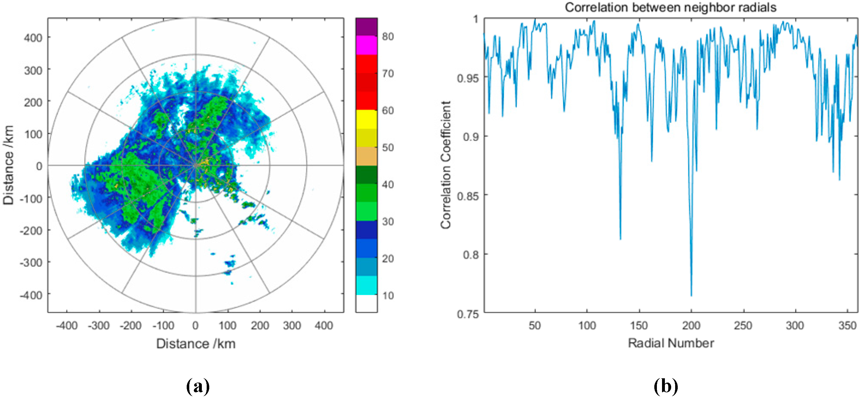
The raw weather radar data contain a substantial amount of spatial redundancy and temporal redundancy. The spatial redundancy contains two types of high degrees of serial correlation. One is the high degree of serial correlation between range bin values in a radial. Consecutive range bins with the same value form runs can be reduced by the RLE (Run length encoding) coding algorithm. The image data for most WSR-88D base products and radial-format-derived products were packed in a 4-bit RLE format [25,26]. The other is the high degree of serial correlation in adjacent radials in volume data. Taking CINRAD SA Radar as an example, the volume data has 360 radials that were sampled at 1° azimuths in an elevation cut. There is strong spatial correlation in neighbor radials, which means that there is similar value distribution in neighbor radials in an elevation cut. This type of spatial redundancy can be utilized by the differential encoding algorithm or prediction algorithm. Figure 2a is a weather radar reflectivity PPI, which has 360 radials sampled at 1° azimuths. Figure 2b shows the correlation coefficients between two neighbor radials in reflectivity data. The value of most correlation coefficients is close to 1. It means that the values for most range bins between neighbor radials are very similar. Most of the information in the current radial can be predicted from the adjacent radial. In addition, the current radial can be fully reconstructed by simply transmitting the residual data between current radial and adjacent radial. The residual data is obtained using differential encoding or prediction, stored using entropy coding. If the prediction between current radial and the reference radial is accurate, the spatial redundancy in the radials can be largely removed. In the condition, the residual would be close to the memoryless source. According to the Shannon coding theorem, the minimal average code length is determined by the zero-order entropy of memoryless source. The probability distribution of residual fits well with Laplace distribution and the zero-order entropy of residual is lower than the raw data [27].
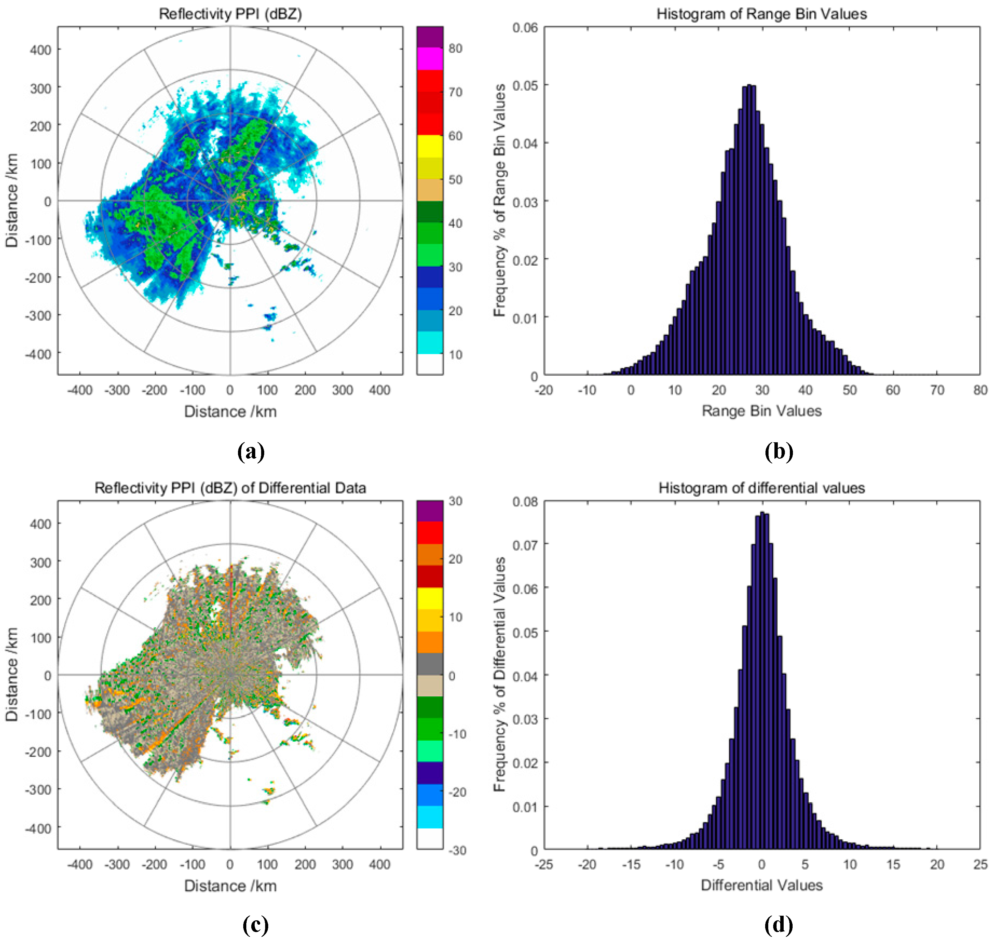
Figure 3a shows the reflectivity PPI of CINRAD SA data, while Figure 3b shows the frequency histogram of range bin values in raw data. The precision of CINRAD reflectivity data is 0.5 dBZ. 48.87% of range bins in the data are represented as missing data. 99.53% of the range bin values are distributed in the range of [−10, 60], and can be represented by 140 symbols. Some lossless compression algorithms (such as differential encoding and linear prediction) can alter the distribution of range bins values. A more concentrated range distribution of data means that the data can be more efficiently compressed. The differential range bins can be calculated, as following:
where Di is the differential value of i-th radial; Ri is i-th radial in raw data; and, Ri−1 is previous radial of Ri in raw data. Differential encoding reduces the dynamic range of data by differentiating adjacent radial data. These methods only change data structure and the decoder can perfectly reconstruct the radials. Figure 3c shows the reflectivity PPI of differential CINRAD SA data. Figure 3d shows the frequency histogram of differential range bins values. In this histogram, 96.34% of the differential values varies in the range of [−20, 20], and can be represented by 80 symbols. There is strong correlation between adjacent radials, which can be efficiently compressed using differential encoding. The structure of differential values has better compression performance using entropy coding than raw data. One of the major drawbacks to differential encoding is the significant degradation in the edge area of echo signal and the area with large amplitude changes. As seen in Figure 3c, the differential coding in the edge area results in larger difference values. The prediction algorithm can be introduced to solve this problem and promote data compression ratio.
2.3. Temporal Redundancy
The raw weather radar data also contains two types of temporal redundancy. The temporal redundancy is related to the volume coverage pattern. Two typical VCPs were widely used in the weather radar. VCP 11 provides 14 unique elevation scans covering elevation angles of 0.5°–19.5° in 5 min. VCP 21 provides nine unique elevation scans between the same lower and upper limits in 6 min. For both of the VCPs, the difference between each of the lowest five elevation angles is 0.95°. The difference increases at higher elevation angles [28]. As most of the weather phenomena is a slow change process, the signal that is sampled at a close time and approximate spatial position contains temporal redundancy. One type of temporal redundancy includes the elevation cuts correlation in the neighbor elevation angles in a volume. The other includes the elevation cuts correlation at the same elevation angle in neighbor volumes. Table 1 shows the correlation of the elevation cuts between five neighbor elevation angles in a volume. The weather radar data tested are the reflectivity CINRAD SA files from China Meteorological Administration. The data files were randomly selected by day and hour at the station 9200 in Guangzhou. The data’s VCP is VCP 21.
Table 1 shows that there is a strong correlation between the elevation cuts at adjacent elevation angles. As the elevation angle increases, the correlation decreases sharply due to the geometric distortion caused by the elevation difference. The matching algorithm can correct geometric distortions between elevation angles.
Table 2 shows the elevation cuts correlation coefficient (CC) between the volume at 7:48 and neighbor volumes at the same elevation angle. The correlation in volumes is significantly stronger than the correlation in elevation cuts at different elevation angles, because there is no geometric distortion. Both the forward data and the subsequent backward data have strong correlation, but in order to ensure real-time coding, only the forward data can be used for prediction coding. In addition, the temporal correlation also drastically decreases with increasing intervals. Prediction using less neighboring data can effectively reduce the computational complexity of the encoder.
3. Proposed Approach
3.1. Lossless Compression Flow
In this paper, the data compression method concentrates on reflectivity product, although similar compression technology can also be applied for other raw moments, such as velocity, spectrum width, differential reflectivity, correlation coefficient, and differential phase.
The preprocessing step is applied to remove the trailing missing data from radials at the beginning. This step reduces the amount of raw data and increases the encoding speed. It is a lossless step because the radials can be fully reconstructed by the decoder using the size of radials from header information. The preprocessing step is specific to weather radar data due to a large number of trailing missing data in weather radar data.
The radar data are transmitted in packets of radials (typically 50 radials at a time) instead of complete volume scans to avoid a systematic delay in the transmission of data [29]. The volume data is processed in units of radials. Each radial is divided into blocks (corresponding to 1 × 16 range bins in the raw radial) for encoding. Block-based processing is conducive to reducing the coding system delay and improving the accuracy of prediction.
Prediction coding is used to reduce the spatial and temporal redundancy in weather radar data. Prediction uses the residual between the current block and predicted block instead of the raw value of current block. Usually, the dynamic range of residual is smaller than the raw data. The decoder can reconstruct the raw block by adding the residual to the block, which is indicated by the motion vector in the reference radial. Prediction outperforms differential encoding, especially in the area where the range bin values are large changes that must be represented outside of the difference byte range.
Entropy coding is a lossless encoding process according to the source entropy. Run-length encoding (RLE) and variable-length coding (VLC) are two widely-used entropy coding techniques. In the paper, the VLC are used for encoding the residual and motion vector of the predicted block to reduce the redundancy. RLE is widely used in weather radar data compression, but the size of radial data may expand by RLE if the radial contains a small number and size of runs of data. The VLC is an entropy coding, which allows for different blocks to be encoded with different numbers of bits. The range bins can be encoded in a few bits or a byte, while the range bins in raw data are represented in bytes. More frequent source symbols are assigned shorter codewords and vice versa. The average bit rate is reduced by VLC. The encoded bit stream is packed in full 8-bits byte for transmission or storage, but the bytes themselves have no intrinsic meaning. Entropy coding techniques determine the number of bits that are assigned to each symbol by the symbol’s frequency of occurrence. Coding efficiency is determined by the value range of symbol. Usually, the distribution of residual data and motion vectors of weather radar data are in a small range and there are many zeros clustering together. Thus, VLC can compress the data effectively.
The work flow of STPC is shown as Figure 4.
- Preprocess the raw data, eliminating the trailing missing data. The purpose of the procedure is to reduce the amount of data just received.
- The redundancy between radials is reduced by using spatial prediction, while the redundancy between volumes can be removed by using temporal prediction.
- The mode selection algorithm selects better by comparing the performance of the two prediction methods.
- The residuals and motion vectors are encoded using entropy coding to compress the data redundancy.
- Adaptive arithmetic algorithm is applied to encode the other data (such as header information).
3.2. Prediction Coding
The prediction technique takes advantage of the weather radar data with its extremely high spatial and temporal correlation. Radial Prediction creates a prediction model from one or more previously encoded radials. The model is formed by shifting range bins in the reference radial(s). The prediction uses block-based prediction and the radial is segmented into blocks. According to the characteristics of weather radar data, the block size is 1 × 16. It means that a block contains 16 continuous range bins in current radial. Each block in current radial is predicted from an area of the same size in a reference radial. The offset between the two areas is the motion vector. The difference between the current block and the predicted block is the residual. The raw data can be completely represented by residual data and motion vectors. If the reference radial and the current radial are in an elevation cut, the prediction mode is spatial prediction. If the reference radial and the current radial in the same elevation and in different volumes, the prediction mode is temporal prediction. In order to ensure the real-time compression algorithm, the reference radial must be encoded in radials.
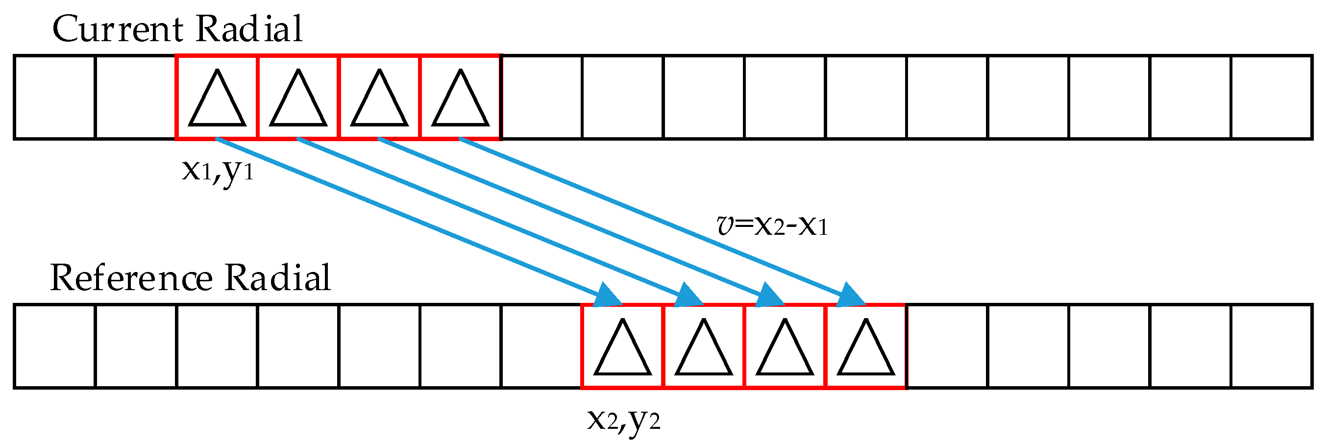
Figure 5 shows the prediction processing between the current radial and reference radial. Motion estimation is used to search for the best matching block in the encoded radial (reference radial) to save the offset of the matching block (motion vector). The criteria for the best matching block involve the minimization of the sum of absolute difference (SAD) between the current block and the predicted block. The SAD of a block is calculated as follows:
where C(i) is i-th range bin in current block and P(i) expresses the i-th range bin in the predicted block. The current block is at the location of (x1,y1) and the best matching block is at the location of (x2,y2). The coordinate x is the number of range bin in a radial, while the coordinate y is the radial index. The motion vector is the offset between the current block and best matching block in coordinate. The motion vector contains the offset in x coordinate and radial index with multi-reference radials applied. The value range of motion vector is determined by the search range and the number of reference radials. The number of reference radials affects the compression performance. More reference frames and a wider search range improves the prediction accuracy, but also requires more computation. In the spatial prediction mode, the reference radials are the previous radials of current radial in an elevation cut. In temporal prediction mode, the reference radials are the radial in the same position of current radial in previous volume and its neighbor radials.
The xi,j of current range bin at the location of pi,j, which denotes the i-th radial in one elevation cut of the weather radar data, is represented using the prediction, as:
where i and k are the number of radial in the elevation cut; j and l expresses the number of range bins in the radial; vn is the motion vector that indicates the direction from i-th radial to k-th radial and forms j-th range bin to l-th range bin, with the range bins in a block having the same motion vector; rn is the residual value that is the range of the bins difference between current block and predicted block; and, vn and rn are prediction coefficients, which are used to replace the raw range bin value xi,j for transmission and storage.
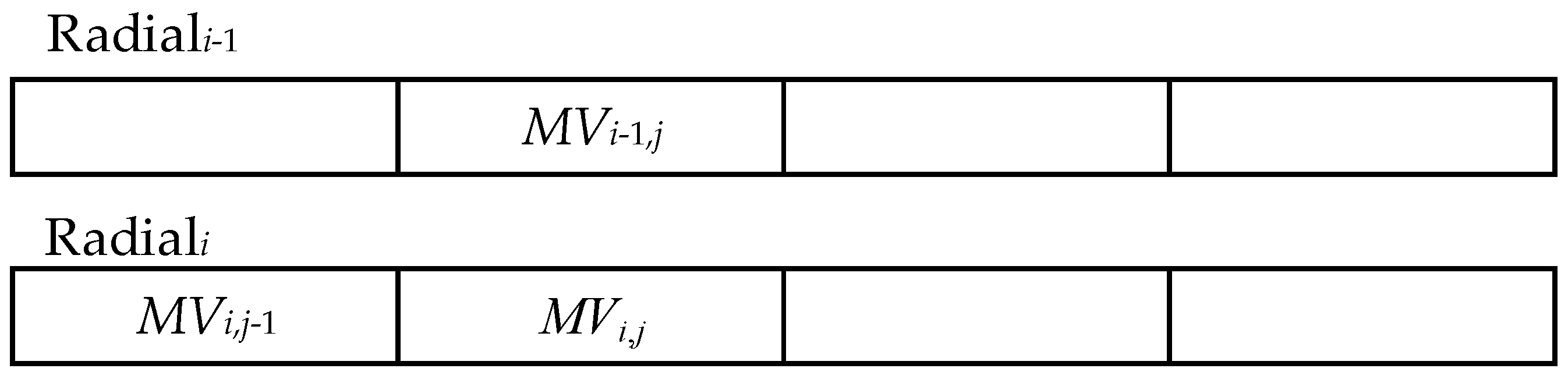
Encoding the MV requires a large number of bits. The motion vector of current block can be predicted from the motion vector of the previously encoded block because the motion vectors between neighbor blocks are often highly spatially correlated. A predicted vector, MVp, is formed based on previously calculated motion vectors and the same position block in the previous radial. Motion vector difference (MVD) is the difference between the current vector and the predicted vector. MVD is encoded and transmitted instead of MV. The method of forming the prediction MVp depends on the motion compensation block and on the availability of nearby vectors. Figure 6 shows positional relationship between the MV used for prediction and the current MV. The MVD is calculated as:
where i is the radial number and j is the j-th block in a radial. MVD contains two parameters: radial index offset and range bin offset.
3.3. Entropy Coding
The residual has a smaller dynamic range than raw data, and thus, can be efficiently replaced by fewer symbols. LZW coding is applied for the residual and MVD. LZW coding uses a variable-length coding table to encode a source symbol, wherein the variable-length coding table is obtained through evaluating the probability of occurrence of symbols. The symbol with high probability use shorter codes, while lower ones use longer codes. It is a lossless compression algorithm that reduces the average length of data.
4. Testing and Results
The data tested is the Level-II S-band CINRAD SA data from China Meteorological Administration. The data files were randomly selected at the station 9200 in Guangzhou. The data products have 460 range bins for each of the 360 radials in an elevation cut.
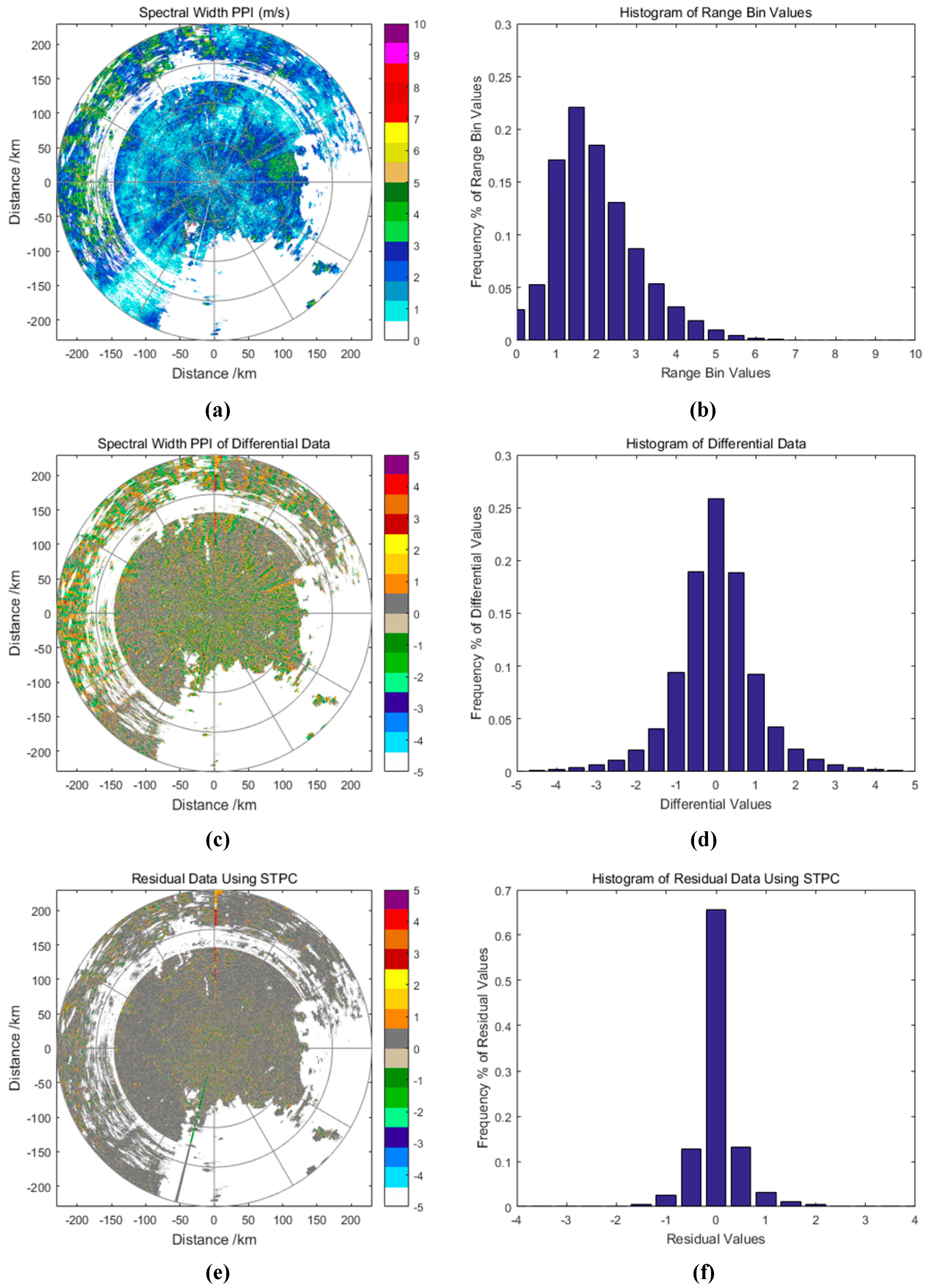
Figure 7, Figure 8 and Figure 9 shows that the reflectivity, radial velocity and spectral width residual and their frequency histogram of CINRAD data, which is used in Figure 3 using different prediction modes. Figure 7 shows that the dynamic range of residual values is decreased using prediction. The absolute value of residual data using SPTC is significantly reduced, while the residual becomes sparser and has more zero values, which are beneficial for a higher compression ratio. The spatial and temporal redundancy can be effectively reduced using SPTC. The histograms show that the distribution of residual values is clustered around the zero value. Using STPC, 99.59% of the residual values are distributed in [−5, 5]. This data structure is suitable for variable length coding, because a higher probability of occurrence of values that are near zero can be encoded with a shorter codeword to reduce the average code length. Compared with the radial-to-radial difference, STPC has a better performance on the region of large amplitude variation. SPTC is based on the prediction of data, while the strong spatial and temporal correlation of weather data is the basis of accurate prediction. Figure 8 and Figure 9 show that STPC is still valid for radial velocity and spectral width data with significantly improved performance for radial-to-radial difference approach.
Table 3 shows the entropy of raw elevation cut and the entropy of residual using different prediction mode. The entropy of the predicted residual is obviously lower than that of the raw data and the differential data. Prediction can effectively remove the redundancy in the data, reduce the entropy of the data, and provide the probability to improve the compression ratio. However, the increase of the entropy caused by the motion vector is not considered in this present study.
In the experiment for the compression efficiency of STPC, sixty volumes data from CINRAD data were selected randomly for the compression experiment. The general-purpose compression programs Bzip2, Gzip, WinZip, and a weather-specific compression scheme, called linear prediction (LP) [29], were compared with STPC in terms of compression size. Bzip2 is a compression method based on block sorting, while Gzip uses arithmetic coding, including Lempel-Ziv and Huffman coding. The motion search was set in a range of [−16, 16] range bins for the reference radial in STPC. Four reference radials are used for each radial, which includes one spatial reference radial (the previous radial of current radial) and three temporal radials (the radial in the same position of current radial in previous volume, its previous radial and its following radial). Table 4 shows that the proposed method achieved the highest compression and the compression ratio reached 7.87. The high compression ratio contributes to the prediction removing the correlation in the data. The data structure of residual and motion vectors is easier to compress than raw data.
5. Conclusions
These results prove the outstanding performance of STPC for Level-II weather radar data. Prediction is an efficient lossless compression method for weather radar level-II data. Results have shown that STPC achieves a higher compression ratio than generic off-the-shelf compression programs and meets the requirement of real-time processing. The compression method can be applied to the storage of super-resolution weather radar data and data communication in a multi-radar network.
The weather radar data is different from the image or video data. Due to the radar detection system, a large amount of invalid data in the weather radar data is defined as missing data. The weather radar data structure makes the compression easier and the amount of data processed is significantly less than the video data, which allows for the weather radar data compression algorithms to easily meet real-time processing requirements. Lossy compression algorithms can further increase the compression ratio of weather radar data. The quantization technology can further promote the compression rate, but also lead to the quantization error, which will affect the quality of the weather radar products generated by the base data. According to different application requirements, designing corresponding lossy compression algorithms still requires significant work.
Acknowledgments
This work was supported by Natural Science Foundation of China (41405030, 41375043, 41575022) and China Scholarship Council (201608515109), Project of Sichuan Province (13Z213), Project of Chengdu University of Information Technology (KYTZ201307, J201503).
Author Contributions
Q.Z., J.H. conceived and designed the numerical experiments; Q.Z., Z.S. designed the compression method; Z.S. performed the numerical experiments; Q.Z., J.H. and X.L. analyzed the results; Q.Z. wrote this paper.
Conflicts of Interest
The authors declare no conflict of interest.
References
- Im, E.; Smith, E.A.; Chandrasekar, V.C.; Chen, S.; Holland, G.; Kakar, R.; Tripoli, G. Workshop Report on NEXRAD-In-Space—A Geostationary Satellite Doppler Weather Radar for Hurricane Studies. In Proceedings of the AMS 33rd Radar Meteorology Conference, Cairns, Australia, 6–10 August 2007. [Google Scholar]
- Lewis, W.E.; Im, E.; Tanelli, S.; Haddad, Z.; Tripoli, G.J.; Smith, E.A. Geostationary Doppler Radar and Tropical Cyclone Surveillance. J. Atmos. Ocean. Technol. 2011, 28, 1185–1191. [Google Scholar] [CrossRef]
- Li, X.H.; He, J.X.; Wang, C.Z.; Tang, S.X.; Hou, X.Y. Evaluation of Surface Clutter for Future Geostationary Spaceborne Weather Radar. Atmosphere 2017, 8, 14. [Google Scholar] [CrossRef]
- Droegemeier, K.; Kelleher, K.; Crum, T.; Levit, J.; Del Greco, S.; Miller, L.; Sinclair, C.; Bennar, M.; Fulker, D.; Edmon, H. Project CRAFT: A test bed for demonstrating the real time acquisition and archival of WSR-88D base (level II) data. In Proceedings of the Conference on Interactive Information and Processing Systems (IIPS) for Meteorology, Oceanography, and Hydrology AMS, Orlando, FL, USA, 13–17 January 2002; pp. 1–4. [Google Scholar]
- Kelleher, K.; Droegemeier, K.; Levit, J.; Sinclair, C.; Jahn, D.; Hill, S.; Mueller, L.; Qualley, G.; Crum, T.; Smith, S.; et al. Project CRAFT: A real-time delivery system for NEXRAD level II data via the Internet. Bull. Am. Meteorol. Soc. 2007, 88, 1045–1057. [Google Scholar] [CrossRef]
- Droegemeier, K. Real-Time Acquisition and Archival of WSR-88D Base Data; University Corporation for Atmospheric Research: Boulder, CO, USA, 2000. [Google Scholar]
- Lakshmanan, V.; Smith, T.; Hondl, K.; Stumpf, G.; Witt, A. A real time, three dimensional, rapidly updating, heterogeneous radar merger technique for reflectivity, velocity and derived products. Weather Forecast. 2006, 21, 802–823. [Google Scholar] [CrossRef]
- Zhang, Q.; Sun, J.; Zhao, C.C.; Chen, H.Y. Development and application of integrated monitoring platform for the Doppler Weather SA-BAND Radar. In IOP Conference Series: Earth and Environmental Science; IOP Publishing: Bristol, UK, 2017; Volume 86. [Google Scholar]
- Wallace, G.K. The JPEG still picture compression standard. IEEE Trans. Consum. Electron. 1992, 38, 18–34. [Google Scholar] [CrossRef]
- Christopoulos, C.; Skodras, A.; Ebrahimi, T. The JPEG2000 still image coding system: An overview. IEEE Trans. Consum. Electron. 2000, 46, 1103–1127. [Google Scholar] [CrossRef]
- Ma, K.; Li, C.Y.; Li, H.Z. A New Hybrid Data Compression Algorithm for Weather Radar. In Proceedings of the 2016 11th International Symposium on Antennas, Propagation and EM Theory (ISAPE), Guilin, China, 18–21 October 2016; pp. 886–889. [Google Scholar]
- Ai, W.H.; Huang, Y.X.; Song, Z.L. Weather radar data compression with parallel adaptive coding algorithm. In Proceedings of the International Congress on Image and Signal Proessing (CISP), Sanya, China, 27–30 May 2008; pp. 197–200. [Google Scholar]
- Vishnu, V.M.; Pravas, R.M. Extreme Compression of weather radar data. IEEE Trans. Geosci. Remote Sens. 2007, 45, 3773–3783. [Google Scholar]
- Mishra, K.V.; Kruger, A.; Krajewski, W.F. Compressed Sensing Applied to Weather Radar. In Proceedings of the 2014 IEEE International Geoscience and Remote Sensing Symposium (IGARSS), Quebec City, QC, Canada, 13–14 July 2014; pp. 1832–1835. [Google Scholar]
- Kawami, R.; Hirabayashi, A.; Tanaka, N.; Shibata, M. 2-Dimensional High-Quality Reconstruction of Compressive Measurements of Phased Array Weather Radar. In Proceedings of the Asia-Pacific Signal and Information Processing Association Annual Summit and Conference (APSIPA), Jeju, Korea, 13–16 December 2016. [Google Scholar]
- Kawami, R.; Hirabayashi, A.; Ijiri, T. 3-Dimensional Compressive Sensing and High-Quality Recovery for Phased Array Weather Radar. In Proceedings of the International Conference on Sampling Theory and Applications (SampTA), Tallin, Estonia, 3–7 July 2017; pp. 658–661. [Google Scholar]
- Seward, J. Bzip2. Available online: www.bzip.org (accessed on 8 March 2018).
- Gailly, J.; Adler, M. The gzip home page. Available online: www.gzip.org (accessed on 8 March 2018).
- Ziv, J.; Lempel, A. A universal algorithm for sequential data compression. IEEE Trans. Inf. Theory 1977, 23, 337–343. [Google Scholar] [CrossRef]
- Lakshmanan, V. Overview of Radar Data Compression. In Proceedings of the Satellite Data Compression, Communications, and Archiving III, San Diego, CA, USA, 19 September 2007; Volume 6683. [Google Scholar]
- Kruger, A.; Krajewski, W.F. Efficient Storage of Weather Radar Data. Softw.-Pract. Exp. 1997, 27, 623–635. [Google Scholar] [CrossRef]
- Kruger, A.; Krajewski, W.F.; Seo, D.J.; Breidenbach, J.P. Development of a large radar database for hydrometeorological studies. In Proceedings of the 29th International Conference on Radar Meteorology, Montreal, QC, Canada, 12–16 July 1999; pp. 945–948. [Google Scholar]
- McCarroll, S.; Yeary, M.; Hougen, D.; Lakshmanan, V.; Smith, S. Approaches for Compression of Super-Resolution WSR-88D Data. IEEE Geosci. Remote Sens. Lett. 2011, 8, 191–195. [Google Scholar] [CrossRef]
- Ai, W.H.; Yan, W.; Li, X. Efficient Lossless Compression of Weather Radar Data. Int. J. Environ. Chem. Ecol. Geol. Geophys. Eng. 2009, 3, 212–215. [Google Scholar]
- National Weather Service, Radar Operations Center. Interface Control Document for the RPG to Class 1 User; Document 2620001C; Radar Operations Center: Norman, OK, USA, 2008. [Google Scholar]
- AWIPS Application Integration Framework Manual; National Weather Service: Chicago, IL, USA, July 2001.
- Shannon, C.E.; Gallager, R.G.; Berlekamp, E.R. Lower bounds to error probability for coding on discrete memoryless channels. Inf. Control 1967, 10, 65–103. [Google Scholar] [CrossRef]
- Brown, R.A.; Steadham, R.M. New WSR-88D Volume Coverage Pattern 12: Results of Field Tests. Weather Forecast. 2005, 20, 385–393. [Google Scholar] [CrossRef]
- Lakshmanan, V. Lossless coding and compression of radar reflectivity data. In Proceedings of the 30th International Conference Radar Meteorology, Munich, Germany, 19–24 July 2001; pp. 50–52. [Google Scholar]
Figure 1.
Missing data statistics of an example CINRAD elevation cut. The tested data is the first elevation cut of the CINRAD SA radar on 20 May 2016 at 07:48 a.m., which has 360 radials in an elevation cut. Each radial has 460 range bins.
Figure 1.
Missing data statistics of an example CINRAD elevation cut. The tested data is the first elevation cut of the CINRAD SA radar on 20 May 2016 at 07:48 a.m., which has 360 radials in an elevation cut. Each radial has 460 range bins.
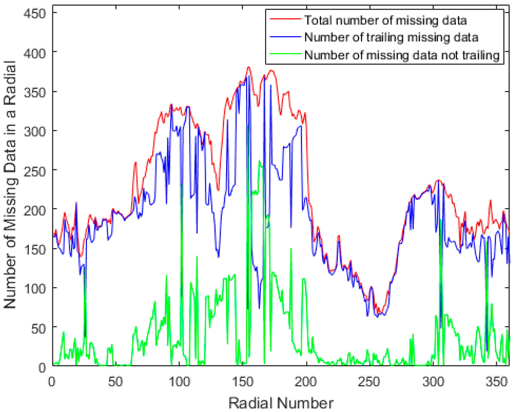
Figure 2.
Reflectivity Plan Position Indicator (PPI) of CINRAD SA data and its spatial correlation in neighbor radials. (a) Reflectivity PPI of CINRAD SA data. The tested data is the first elevation cut of the CINRAD SA radar on 20 May 2016 at 07:48 a.m.; and, (b) the statistics of the correlation coefficients between neighbor radials.

Figure 3.
The distribution of raw data and differential data. The differential data is calculated by difference between the current radial and its previous radial. (a) Reflectivity PPI (dBZ) of CINRAD SA data; (b) frequency histogram of range bin values in raw data; (c) reflectivity PPI (dBZ) of differential CINRAD SA data; and, (d) frequency histogram of differential range bins values that are calculated from Equation (1).

Figure 4.
Spatial and temporal prediction compression (STPC) Flow.
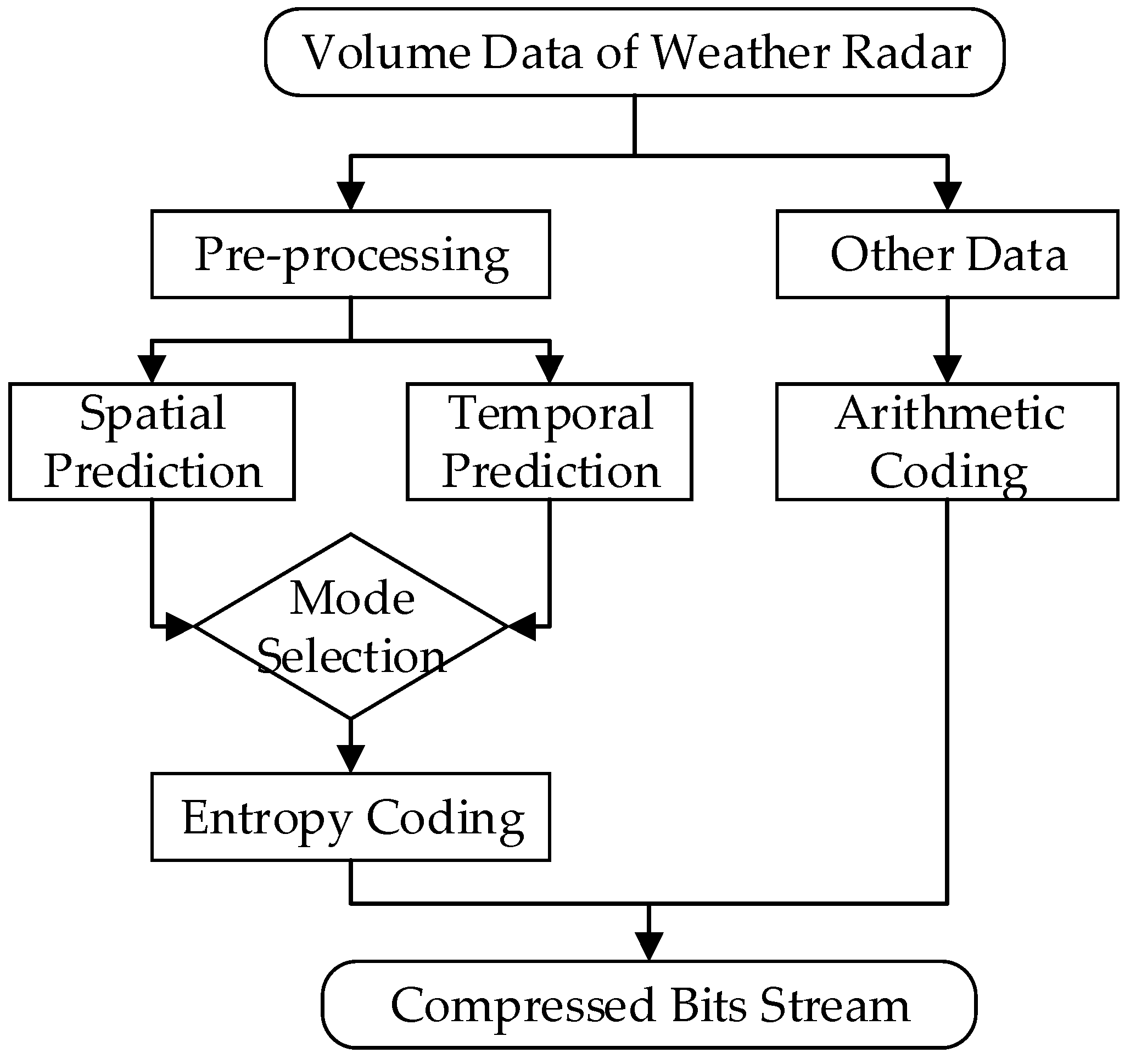
Figure 5.
Prediction between radials.

Figure 6.
Calculation of the predicted motion vector.

Figure 7.
Residual and frequency histogram of range bin values for CINRAD elevation cut using different prediction mode: (a) Residual data using spatial prediction; (b) frequency histogram of residual data using spatial prediction; (c) residual data using temporal prediction; (d) frequency histogram of residual data using temporal prediction; (e) residual data using STPC; and, (f) frequency histogram of residual data using STPC.
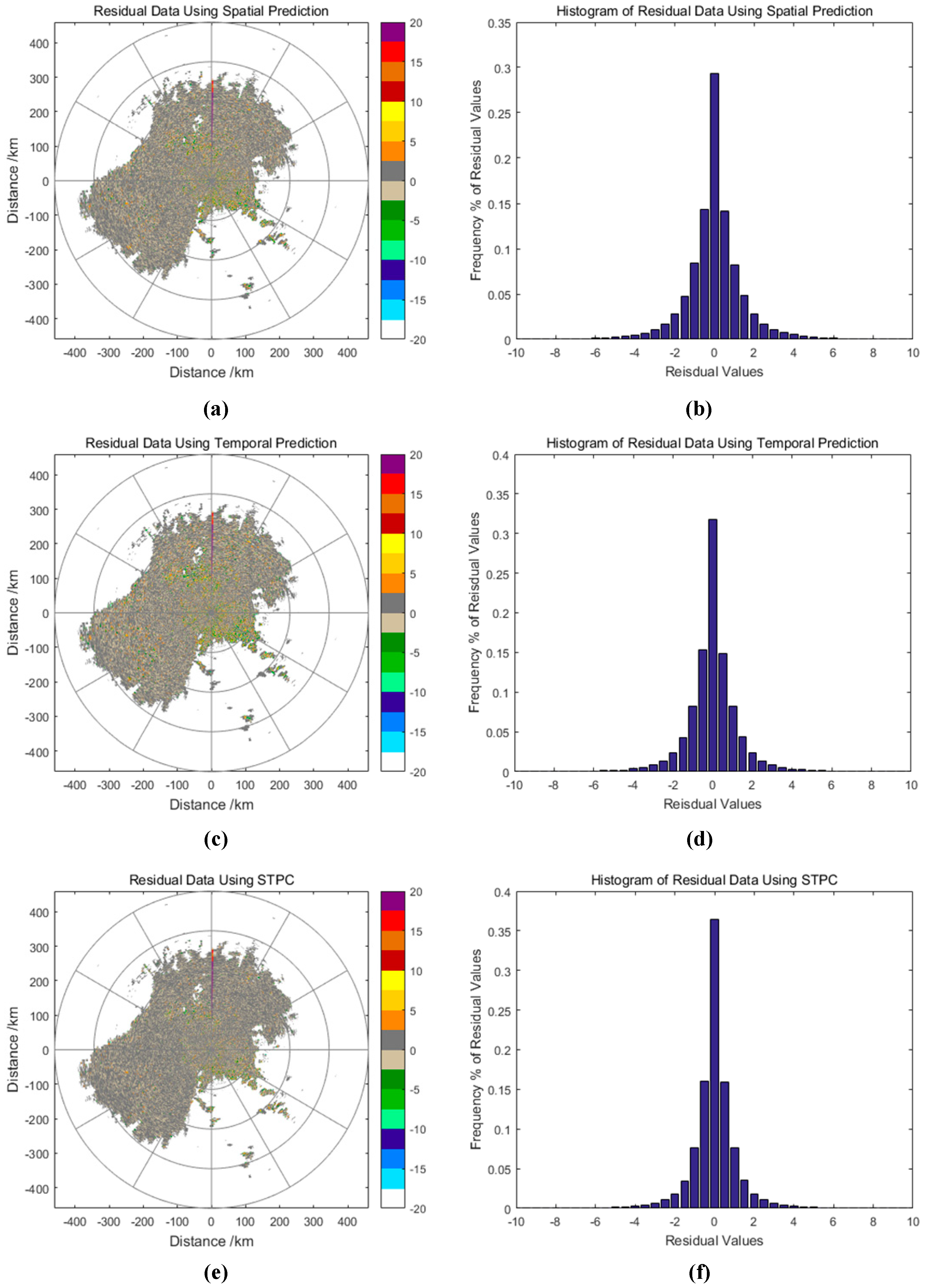
Figure 8.
The distribution of radial velocity data, radial velocity differential data and radial velocity residual data using STPC: (a) Radial velocity PPI of CINRAD SA data; (b) frequency histogram of radial velocity data; (c) radial velocity PPI of differential data; (d) frequency histogram of radial velocity differential data; (e) radial velocity PPI of residual data using STPC; and, (f) frequency histogram of radial velocity residual data using STPC.
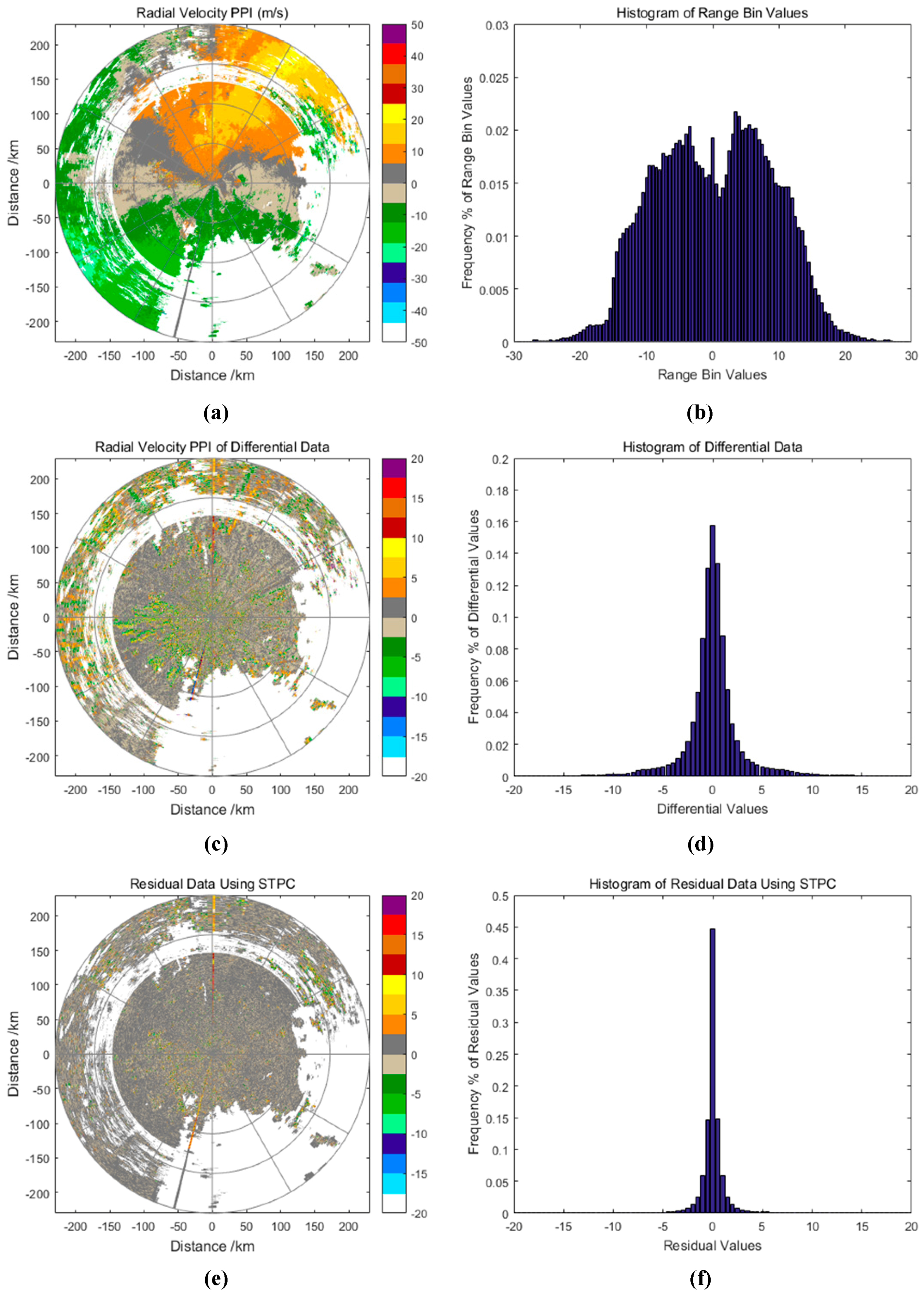
Figure 9.
The distribution of spectral width data, spectral width differential data and spectral width residual data using STPC: (a) Spectral width PPI of CINRAD SA data; (b) frequency histogram of spectral width data; (c) spectral width PPI of differential data; (d) frequency histogram of spectral width differential data; (e) spectral width PPI of residual data using STPC; and, (f) frequency histogram of spectral width residual data using STPC.


Table 1.
Correlation of elevation cuts in neighbor elevation angles in a volume.
| Layer | 1 | 2 | 3 | 4 | 5 |
|---|---|---|---|---|---|
| 1 | 1 | ||||
| 2 | 0.8379 | 1 | |||
| 3 | 0.3115 | 0.8588 | 1 | ||
| 4 | 0.1856 | 0.3719 | 0.8640 | 1 | |
| 5 | 0.0683 | 0.2129 | 0.7337 | 0.8938 | 1 |
Table 2.
Elevation cuts correlation at the same elevation angles in neighbor volumes.
| Time | 7:24 p.m. | 7:30 p.m. | 7:36 p.m. | 7:42 p.m. | 7:48 p.m. | 7:54 p.m. | 8:00 p.m. | 8:06 p.m. | 8:12 p.m. |
|---|---|---|---|---|---|---|---|---|---|
| CC | 0.8780 | 0.8966 | 0.9154 | 0.9428 | 1 | 0.9482 | 0.9142 | 0.8945 | 0.8803 |
Table 3.
Entropy of raw elevation cut and residual using different prediction mode.
| Base Data | Raw Data | Difference | Spatial | Temporal | STPC |
|---|---|---|---|---|---|
| DBZ | 4.60 | 3.58 | 2.53 | 2.38 | 2.21 |
| VEL | 5.46 | 4.35 | 2.88 | 2.96 | 2.72 |
| WID | 3.40 | 3.18 | 1.94 | 1.92 | 1.65 |
Table 4.
Compression ratio of different method.
| Method | Bzip2 | Gzip | Winzip | LP | STPC |
|---|---|---|---|---|---|
| Ratio | 5.82 | 4.93 | 4.88 | 5.67 | 7.87 |
© 2018 by the authors. Licensee MDPI, Basel, Switzerland. This article is an open access article distributed under the terms and conditions of the Creative Commons Attribution (CC BY) license (http://creativecommons.org/licenses/by/4.0/).
Share and Cite
MDPI and ACS Style
Zeng, Q.; He, J.; Shi, Z.; Li, X. Weather Radar Data Compression Based on Spatial and Temporal Prediction. Atmosphere 2018, 9, 96. https://doi.org/10.3390/atmos9030096
AMA Style
Zeng Q, He J, Shi Z, Li X. Weather Radar Data Compression Based on Spatial and Temporal Prediction. Atmosphere. 2018; 9(3):96. https://doi.org/10.3390/atmos9030096
Chicago/Turabian StyleZeng, Qiangyu, Jianxin He, Zhao Shi, and Xuehua Li. 2018. "Weather Radar Data Compression Based on Spatial and Temporal Prediction" Atmosphere 9, no. 3: 96. https://doi.org/10.3390/atmos9030096
Note that from the first issue of 2016, this journal uses article numbers instead of page numbers. See further details here.