Diurnal and Seasonal Variations of Carbon Dioxide (CO2) Concentration in Urban, Suburban, and Rural Areas around Tokyo

Atmosphere and Ocean Research Institute, The University of Tokyo, Kashiwa-shi, Chiba 277-8568, Japan
*
Author to whom correspondence should be addressed.
Atmosphere 2018, 9(10), 367; https://doi.org/10.3390/atmos9100367
Submission received: 20 April 2018
/
Revised: 17 August 2018
/
Accepted: 5 September 2018
/
Published: 20 September 2018
(This article belongs to the Special Issue Greenhouse Gases: Measurements and Analysis)
Abstract
:Site environments and instrumental characteristics of carbon dioxide (CO2) measurements operated by local governments in the Kanto Plain, the center of which is Tokyo, were summarized for this study. The observation sites were classified into environments of three types: urban, suburban, and woodland. Based on a few decades of accumulated hourly data, the diurnal and seasonal variations of CO2 concentrations were analyzed as a composite of anomalies from annual means recorded for each site. In urban areas, the highest concentrations appear before midnight in winter. The second peak corresponds to the morning rush hour and the strengthening of the inversion layer. Suburban areas can be characterized as having the highest concentration before dawn and the lowest concentration during the daytime in summer in association with the activation of respiration and photosynthesis of vegetation. In these areas, concentration peaks also appear during the morning rush hour. Woodland areas show background features, with the highest concentration in early spring, which are higher than the global background by about 5 ppmv.
1. Introduction
Since the 1990s, studies of CO2 emissions and uptake using global scale inverse models [1] have been conducted based on in situ measurements to monitor background levels using data from global meteorological networks [2,3,4]. Source/sink strengths have been evaluated by these studies as a time series on sub-continental scales (e.g., [5]). However, because the number of observation sites are limited, particularly over the ocean, satellite observation of CO2 has been sought for a long time for a more accurate evaluation of phenomena. Responding to this demand, Earth observation satellites such as the greenhouse gases observing satellite (GOSAT) and Orbiting Carbon Observatory-2 (OCO-2), were launched. Ever since, they have been provided global observations [6,7]. Source/sink inverse analyses have also been conducted (e.g., [8]). Recently, regional through city-scale emissions assessment has attracted attention as a target of satellite observations (e.g., [9,10,11]).
In the context of general interest in the global environment, local governments have conducted CO2 observations in each prefecture of Japan. Although it has been expected that these data shall be used to estimate CO2 emissions from large cities in conjunction with satellite data, characterizations of observation sites and data have not been studied synthetically, except for a few studies, despite the datasets having been available to researchers for more than a decade [12].
This study summarizes site locations and instrumental characteristics of CO2 measurements conducted by local governments in the Kanto Plain, Japan. These are the only data officially available in a digital format to researchers for the region. Based on data observed during more than a decade, the diurnal and seasonal variations of CO2 concentrations were analyzed to characterize site environments.
2. Observation Sites, Instruments, and Analysis
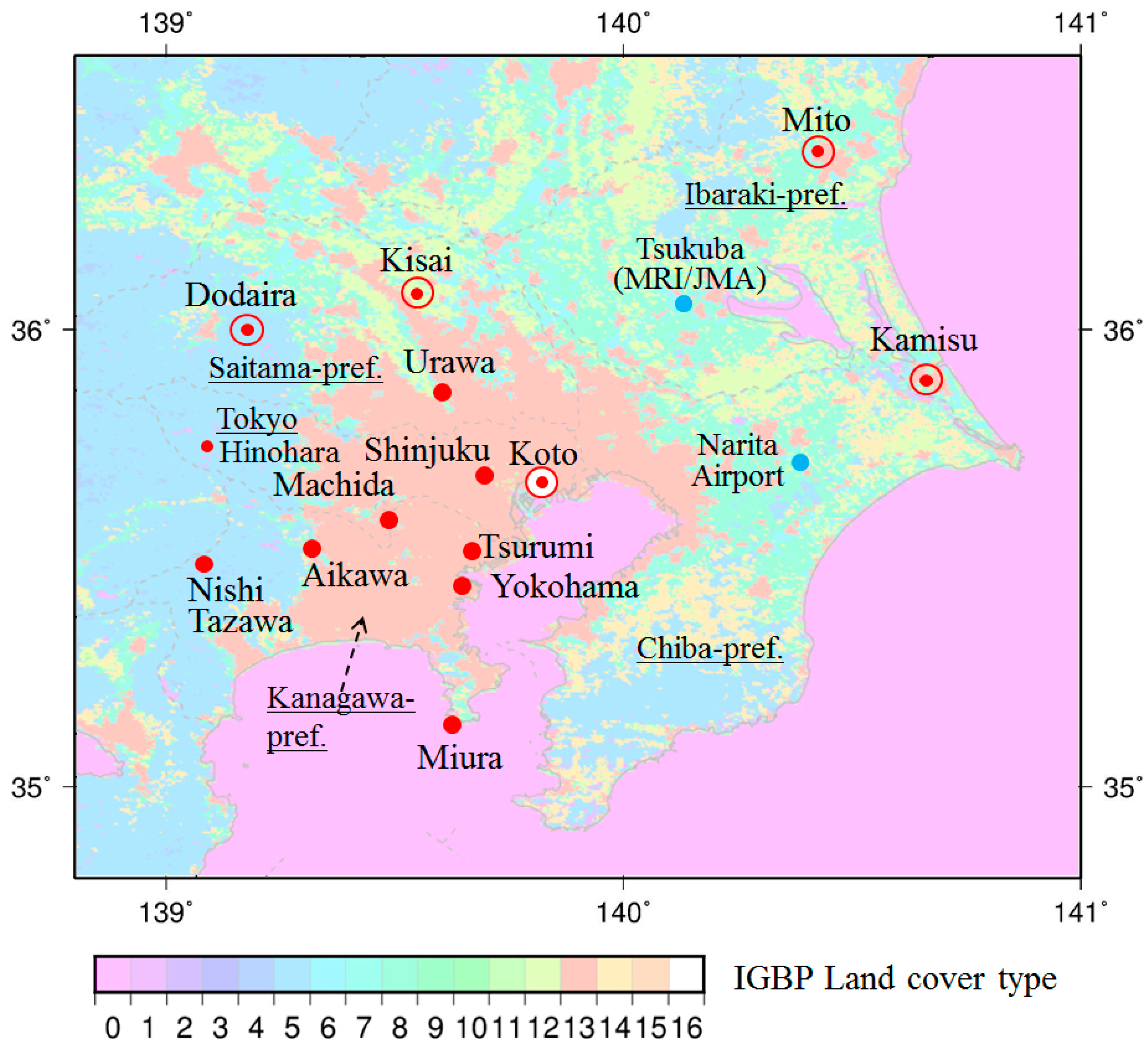
Figure 1 portrays the locations of the observation sites operated by local governments or government-funded research institutes. Names of prefectures are underlined in the figure. Closed red circles with an open circle represent sites for which hourly data are available as digital data for all observation periods. Site information, instrumentation, and results of data analyses are presented for these five sites in this report. Closed red circles represent older sites for which data are no longer provided in digital files. One closed blue circle in Figure 1 denotes the location of the Meteorological Research Institute of the Japan Meteorological Agency (MRI/JMA) where there was a 200 m high tower and where CO2 concentrations had been measured at 1.5 m, 25 m, 100 m, and 200 m heights during 2000–2010 [13]. Another closed blue circle in the figure shows the location of Narita Airport, where vertical profiles of CO2 concentration have been measured by passenger aircraft in conjunction with the Japan Airlines project: the comprehensive observation network for trace gases by airliner (CONTRAIL) [14,15]. For reference, the International Geosphere–Biosphere Programme (IGBP) land cover types based on the standard products of the moderate resolution imaging spectroradiometer (MODIS) data was superimposed as the background color of Figure 1 [16]. In this classification, it is obvious that the “Koto” site is located in the urban area and the “Dodaira” site is in the woodland. “Mito” and “Kisai”, which are classified into suburbs, are in the grass land or cropland near local cities. “Kamisu” is surrounded by grass land and cropland, but the site is just located in a local city.
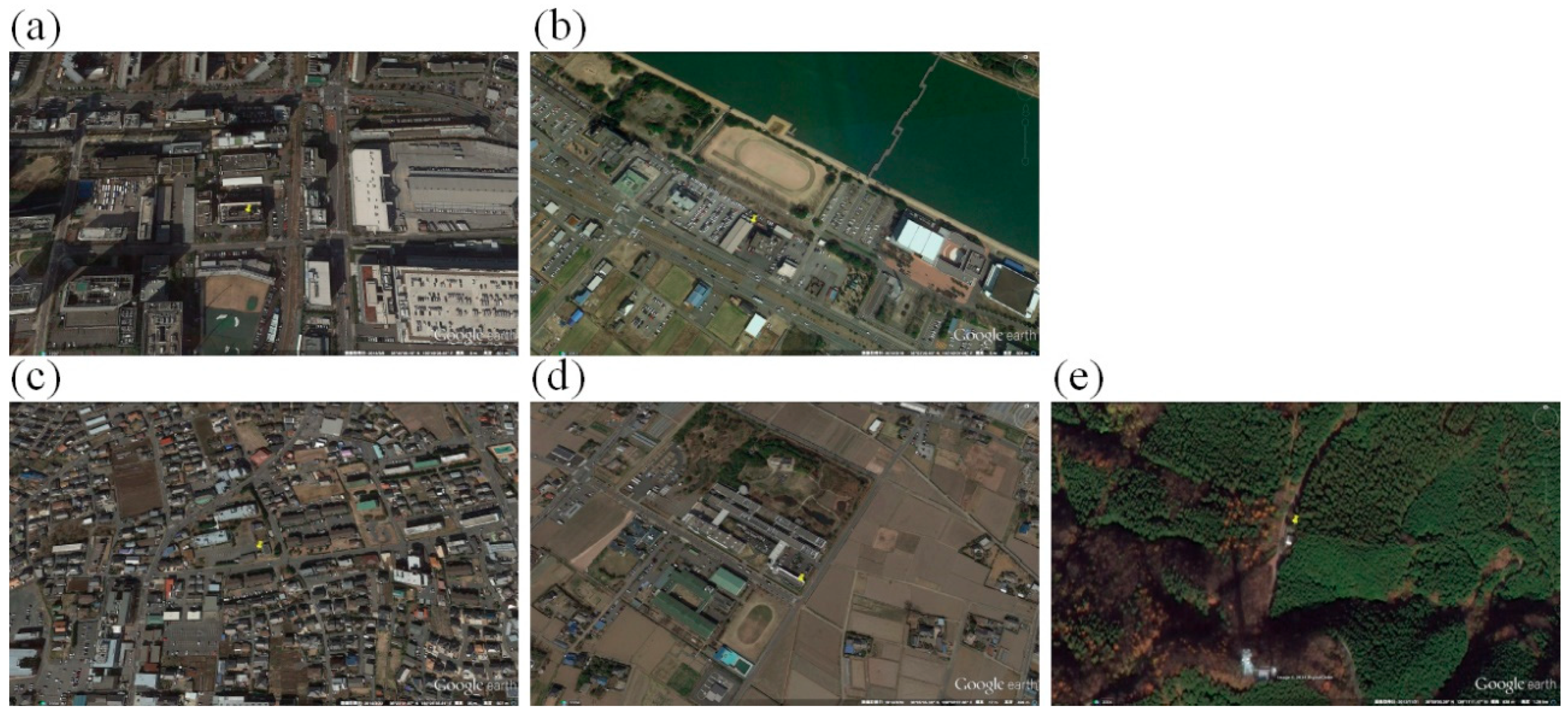
Figure 2 presents aerial photograph of five sites: (a) Koto (Tokyo), (b) Kamisu (Ibaraki), (c) Mito (Ibaraki), (d) Kisai (Saitama), and (e) Dodaira (Saitama). For these sites, hourly data are available as digital data. Judging from photographs and field surveys conducted by the authors, these five sites are classified into environments of three types: urban, suburban, and woodland. Information related to these five sites and instruments is presented in Table 1.
The Tokyo Metropolitan Research Institute for Environmental Protection has conducted CO2 measurements for the Tokyo metropolitan government. Koto is the only site in Tokyo. Measurements there continued through August 2015. Since the site is located in an industrial area near Tokyo Bay, it is classified as an urban area. The measurement system is placed in an upper level of the institute building. The inlet for air sampling is placed at the top of the building. Other observation sites in Tokyo are presented in Figure 1. The measurements were conducted at Shinjuku and Machida during 1993–1998. The Hinohara site was used during 2000–2001.
One site in Ibaraki prefecture, Kamisu, is an urban site located in the Kashima coastal industrial zone. The observation shed is placed in an area used as a fire station. The other site in Ibaraki prefecture is in Mito city. The site is located in a residential area, but the area is only a few kilometers, surrounded by rice paddy fields with some woods. This site can be regarded as suburban. Measurements at these two sites are conducted by the Ibaraki Prefectural Government, but operations have been consigned to a private company.
Kisai in Saitama prefecture is another suburban site. It is surrounded mainly by rice paddy fields, with houses studding the fields. The Dodaira site is located almost at the top of Dodaira Mountain, which is located at the west end of the Kanto Plain. The site is in a woody area with evergreen conifers. Its altitude is 831 m, the highest among the sites. Both sites, Kamisu and Dodaira, have been registered with the World Data Centre for Greenhouse Gases (WDCGG) [4]. Earlier, there was a site at Urawa. It was used during 1991–2002 before measurements started at the Kisai site.
In Kanagawa prefecture there is no observation site for which data are available now, but there were five sites at Tsurumi (operated in 1992–2006), Yokohama (1992–2006), Miura (1992–2006), Nishitanzawa (2000–2006), and Aikawa (2002–2006). During March 1998 through May 2000, measurements using a helicopter were conducted seven times to observe the three-dimensional distribution of CO2 over the cities in Kanagawa prefecture. We investigated official reports and newsletters published by the local government, but no record of CO2 observations exists for Chiba prefecture.
To measure CO2, the non-dispersive infrared absorption (NDIR) system is used at all sites. The model numbers are presented in Table 1. As a procedure common to all systems, the following method was applied to introduce sample air into the system; (1) sample air was introduced into a pile through an inlet (unit for preventing rain) which is placed at the top of a tower (5–20 m height), (2) the air is filtered to remove aerosols, (3) water vapor is removed from the air by a dehumidifier or chemicals, and (4) the air is introduced into the NDIR system. Then, the CO2 concentration of the sample gas was measured using the span gas listed in Table 2. The most important factor affecting its measurement accuracy is the calibration of the instrument. Gas types used for calibration, the CO2 concentration of the reference and span gases, their accuracy, and the frequency of calibration are presented in Table 2. In Saitama prefecture, the secondary gases calibrated by the JMA and their accuracy are evaluated as 0.1 ppmv. They are used for calibrating reference gases. By calibrating the system every 2 h, the representability of measurements is estimated as being better than 0.2 ppmv [18]. In other prefectures, commercially sold gases are used for the calibration. Their concentration accuracy is labeled as 1 ppmv. The calibration frequency is every 13 h at Koto, and one week at Kamisu and Mito. Also affecting the measurement accuracy are the dehumidifier and aerosol filter. Their dew point temperature and filter pore size are presented in Table 1. Although we visited the Kamisu site and read all documents related to the system configuration kept at the office of Ibaraki Prefectural Government, we found no description of the dehumidifier component and aerosol filter of the system.
From all sites, hourly data were distributed to users upon request for disclosure except for the data from Saitama prefecture, which are obtainable from the WDCGG website. For this study, hourly data are simply averaged to obtain daily mean values as long as more than 50% of the data are valid. Monthly mean values are obtained using the same manner of averaging.
3. Results
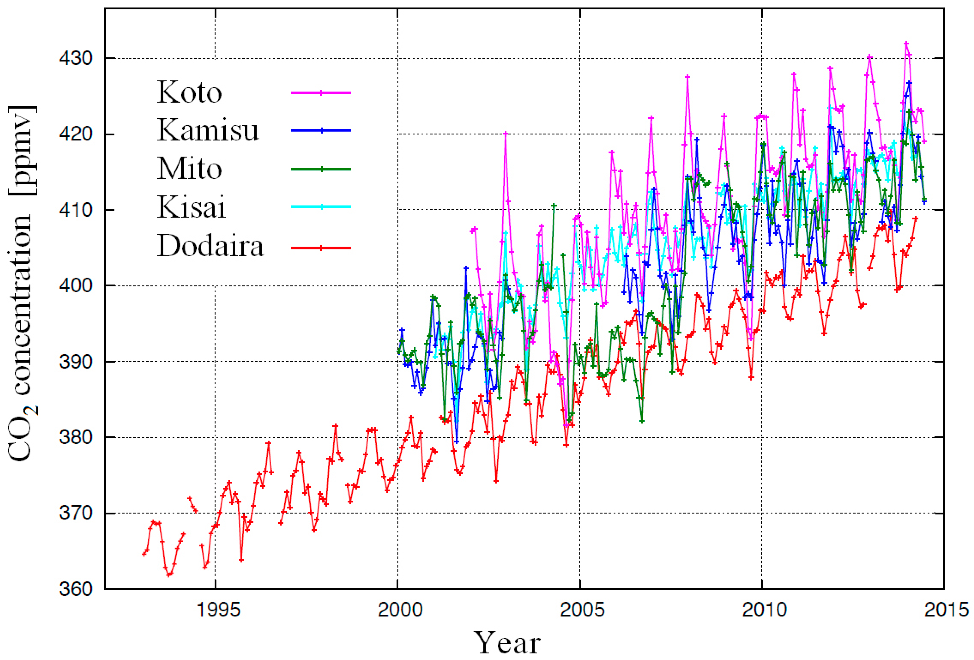
Monthly mean CO2 concentrations for all sites in the Kanto Plain are shown as a function of time in Figure 3. At all sites, concentrations have increased almost constantly, clearly showing the seasonal cycle. The growth rates are uniformly about 2 ppmv/year. The annual mean value is highest at Koto (Tokyo) and lowest at Dodaira (Saitama). At the Mito (Ibaraki) site, the values in 2004–2007 are remarkably smaller than those expected from the trend line compared with other years. Reportedly, the measurement system was replaced in 2004. The system was not well calibrated during the period.
To extract the diurnal and seasonal variations of CO2 concentration at each site, the annual mean value centered at each daily mean with a one-year time window was calculated and substituted from each hourly data point to obtain anomalies. These anomalies were composed as a function of the local time and month for each site. The composited results for all observation periods up to 2014 are presented in Figure 4.
At the Koto site, the highest concentration appears before midnight in winter; the second peak appears at 7–10 a.m. in all seasons (Figure 4a). The daily minimum appears at around 3 p.m. in all seasons, and their lowest concentration has been recorded in September. Kamisu (Ibaraki) is another site classified as an urban area, showing similar features to those of the plot for the Koto site (Figure 4b). However, the highest concentration before midnight in winter is lower than that at the Koto site. Furthermore, the minimum value in August is lower.
Mito (Saitama) and Kisai (Saitama), which are classified as suburban areas, show mutually similar features (Figure 4c,d) These areas can be characterized having the highest concentration before dawn and the lowest concentration in the daytime during summer. At the Mito site, an increase of concentration appeared before midnight, as in urban areas in winter.
Dodaira (Saitama) site is a woodland area. The features of diurnal and seasonal variation differ from those of other sites (Figure 4e). The daily average is highest in springtime and lowest in late summer. Although the scale range of presented values is expanded for the Dodaira site to emphasize the relative variation, the variation amplitude is two or three times lower than those of urban and suburban areas.
4. Discussion
As presented in Section 2, the measurement accuracy differs among sites. In Saitama prefecture, the accuracy and representativity are about 0.2 ppmv using officially released calibration gases. The data screening criteria follows that recommended by WDCGG. On the other hand, the accuracies can be a few parts per million by volume (ppmv) for data observed in Ibaraki prefecture and Tokyo city, mainly because of the low accuracy of calibration gases and low frequency of calibration operation, particularly in Ibaraki prefecture where the calibration frequency is only once per week. However, the room temperature and dehumidifier temperature are kept constant. As it is expected that the measurement systems have not been unstable, measurement accuracies can be on the order of a few parts per million by volume. As a consequence, the measurement accuracy of a few parts per million by volume is achieved and is sufficiently accurate to represent the diurnal and seasonal variations presented in Section 3 because the amplitude of the variation is about 10 times greater than the measurement accuracy.
Many studies have been made to characterize the CO2 concentration or flux in areas of various types classified in the same way as we described as a result of this study [5,19,20,21,22,23,24,25,26,27,28,29,30]. Many of them are made based on CO2 flux measurements using the eddy covariance method, which analyze CO2 concentration data measured with a high response speed system and three-dimensional wind data measured by a ultrasonic anemometer assuming that the vertical gradient of CO2 concentration is proportional to CO2 flux from the surface. The characteristics of concentrations and fluxes proved by this method can show almost identical features to those presented in this study because the concentration is strongly affected by the flux (emission/up take) in a limited spatial and temporal scale.
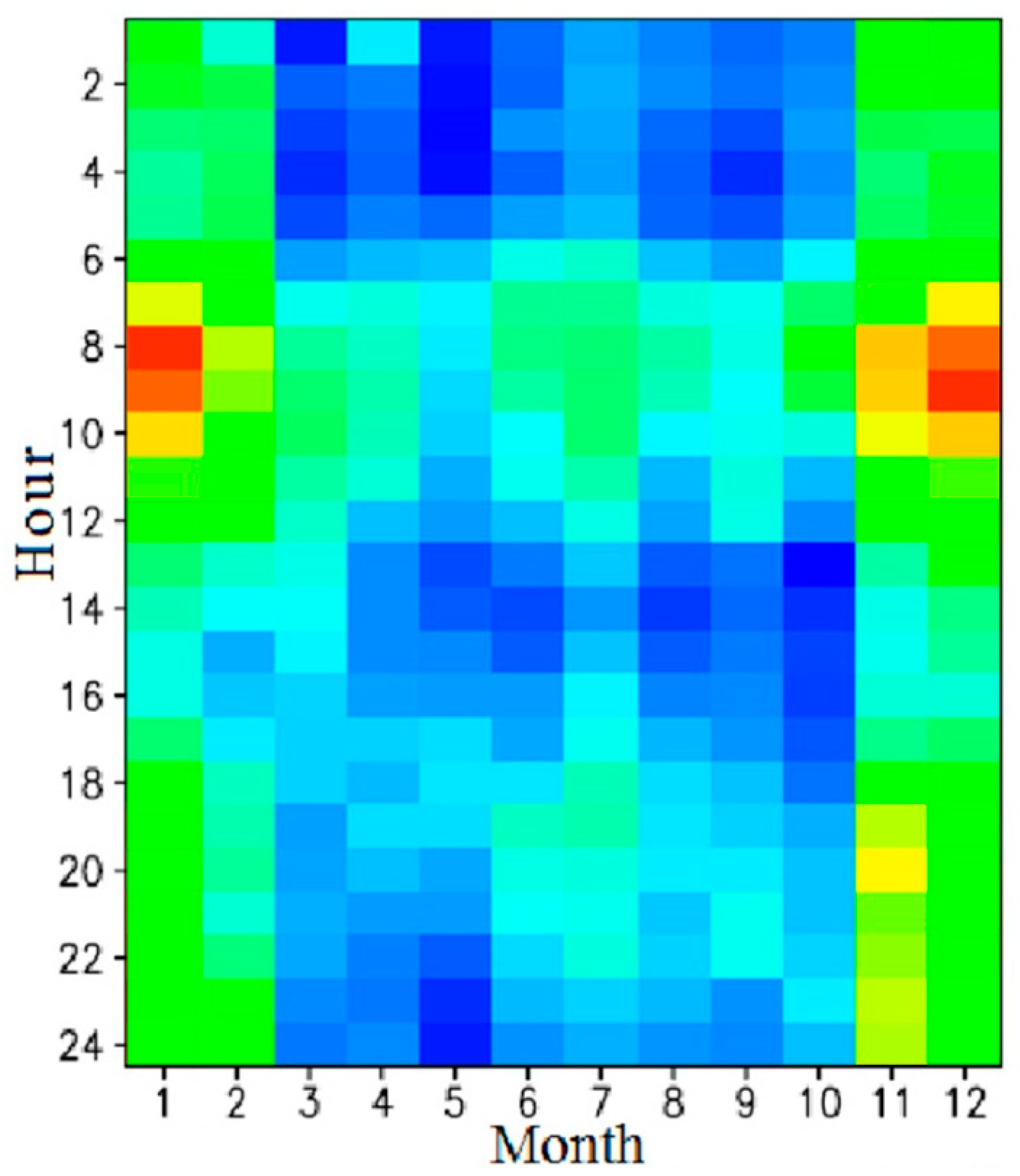
The results of this study demonstrated that urban areas are characterized by high concentrations before midnight in winter and in the morning during all seasons. Many studies conducted for urban areas show similar features. For example, Ward et al. [29] drew a similar plot of the diurnal variation of CO2 concentration in London to show the increase of the concentration during the nighttime in winter, George et al. [21] also showed a similar feature in Baltimore, and Coutts et al. [31] showed both increases in the morning and winter midnight in Melbourne. One can infer that the high concentration before midnight in winter is attributable to emissions from private households, heating, or from businesses [24]. Some reports (e.g., [12]) describe that the increase in CO2 concentration derives from an increase of atmospheric stability during the nighttime. If that is true, then the concentration can be expected to increase constantly up to the time of sunrise. However, the actual concentration shows a decrease immediately after the midnight, then it increases again until sunrise. Therefore, it can be concluded that the increase of CO2 concentration before midnight is mainly attributable to the increase of CO2 emission in this area. On the other hand, high CO2 concentration in the morning is attributable to emissions corresponding to the rush hour [22,31,32]. This can be confirmed from the comparison with nitrogen oxide (NOx) concentration, which is generally a measure of traffic volume. Figure 5 shows the hourly–monthly means of NOx concentration at an observation point near Koto site for 2010. It shows a significant increase of NOx concentration during the morning rush hour time. The peak time and strength of CO2 concentrations corresponded to the features of NOx. The minimum concentration appearing in the daytime in summer at Kamisu is lower than that at Koto because the Kamisu site is surrounded by more vegetation than the Koto site, and CO2 uptake by vegetation around Kamisu site is stronger than that around Koto.
High and low concentrations were respectively found during nighttime and daytime in suburban areas in summer, as reported by some studies for the Mito and Kisai sites [22,33]. They correspond to the respiration and photosynthesis of vegetation in the area.
A smaller amplitude of variation and the highest concentration in spring time are the characteristics of the background concentration of CO2 [2,34]. At the Dodaira site, diurnal and seasonal variations are similar to those of the background, but the average level is higher than the global background by about 5 ppmv [4]. At the Dodaira site, high concentrations of CO2 before drawing have not been observed in spite of the existence of vegetation in the area because the inversion layer near the surface is not easily formed near a mountain top.
To estimate the total amounts of CO2 emissions and uptake precisely, numerical simulation models used for estimation should be able to represent the nature of CO2 concentration not only spatially, but also temporally, as observed. From this perspective, characteristics of the diurnal and seasonal variation of CO2 concentration presented by this study for urban, suburban, and woodland areas around Tokyo can be the standard features presented by the models. However, this study also showed that CO2 concentration characteristics vary depending on the type of the surrounding environment even when the sites are classified into the same type of environment. Therefore, measurements must be made operationally for every site. Nevertheless, measurements at the Koto site stopped in August 2017; no official observation site exists in Tokyo anymore. Since the reduction of CO2 emissions from the city has recently attracted great attention, CO2 measurements are expected to begin again in Tokyo.
5. Conclusions
CO2 measurement sites operated by the local governments in the Kanto Plain have been classified as urban, suburban, and woodland. Characteristics of the diurnal and seasonal variation of CO2 concentration have been presented for the environments of the three types. Although the measurement accuracy varies among prefectures depending on the types of calibration gases and frequency of calibration operation, it is by no means accurate enough to represent the diurnal and seasonal variations presented in this study. This study demonstrated clearly that continuous measurements at fixed observation sites can elucidate the effects of CO2 emissions and uptake around the site. On the other hand, satellite instruments can target arbitrary locations. However, because the observation times are generally limited to around noon, the diurnal cycle of CO2 emission is difficult to observe by satellites. Therefore, it can be inferred that satellite measurement data should be used synergistically with ground-based measurements to estimate CO2 emissions and uptake from a city effectively. Furthermore, comparison with other types of methods to estimate CO2 emissions, such as statistical inventory database building, is necessary to make the results more reliable [35,36].
Author Contributions
R.I. conducted the research and wrote the manuscript; Y.T. carried out the field research and analyzed the data.
Funding
This research received no external funding.
Acknowledgments
CO2 data used for this study were provided by the Tokyo Metropolitan Research Institute for Environmental Protection, Ibaraki prefectural government, and WDCGG. NOx data were provided by the Environmental Department of Tokyo Metropolitan Government. The authors especially thank Yosuke Muto of the Center for Environmental Science in Saitama (CESS) for his valuable comments related to measurement techniques and data analyses.
Conflicts of Interest
The authors declare no conflict of interest.
References
- Gurney, K.R.; Law, R.M.; Denning, A.S.; Rayner, P.J.; Baker, D.; Bousquet, P.; Bruhwiler, L.; Chen, Y.H.; Ciais, P.; Fan, S.M.; et al. Transcom 3 CO2 inversion intercomparison: 1. Annual mean control results and sensitivity to transport and prior flux information. Tellus Ser. B Chem. Phys. Meteorol. 2003, 55, 555–579. [Google Scholar] [CrossRef]
- Conway, T.J.; Tans, P.P.; Waterman, L.S.; Thoning, K.W. Evidence for interannual variability of the carbon-cycle from the national-oceanic-and-atmospheric-administration climate-monitoring-and-diagnostics-laboratory global-air-sampling-network. J. Geophys. Res. 1994, 99, 22831–22855. [Google Scholar] [CrossRef]
- Andrews, A.E.; Kofler, J.D.; Trudeau, M.E.; Williams, J.C.; Neff, D.H.; Masarie, K.A.; Chao, D.Y.; Kitzis, D.R.; Novelli, P.C.; Zhao, C.L.; et al. CO2, Co, and CH4 measurements from tall towers in the NOAA earth system research laboratory’s global greenhouse gas reference network: Instrumentation, uncertainty analysis, and recommendations for future high-accuracy greenhouse gas monitoring efforts. Atmos. Meas. Tech. 2014, 7, 647–687. [Google Scholar] [CrossRef]
- Tsutsumi, Y.; Mori, K.; Ikegami, M.; Tashiro, T.; Tsuboi, K. Long-term trends of greenhouse gases in regional and background events observed during 1998–2004 at Yonagunijima located to the east of the Asian continent. Atmos. Environ. 2006, 40, 5868–5879. [Google Scholar] [CrossRef]
- Baker, D.F.; Law, R.M.; Gurney, K.R.; Rayner, P.; Peylin, P.; Denning, A.S.; Bousquet, P.; Bruhwiler, L.; Chen, Y.H.; Ciais, P.; et al. Transcom 3 inversion intercomparison: Impact of transport model errors on the interannual variability of regional CO2 fluxes, 1988–2003. Glob. Biogeochem. Cycles 2006, 20. [Google Scholar] [CrossRef]
- Crisp, D.; Team, O.C.O. Measuring atmospheric carbon dioxide from space with the orbiting carbon observatory-2 (OCO-2). Proc. SPIE Earth Obs. Syst. 2015, 960702. [Google Scholar] [CrossRef]
- Yoshida, Y.; Ota, Y.; Eguchi, N.; Kikuchi, N.; Nobuta, K.; Tran, H.; Morino, I.; Yokota, T. Retrieval algorithm for CO2 and CH4 column abundances from short-wavelength infrared spectral observations by the greenhouse gases observing satellite. Atmos. Meas. Tech. 2011, 4, 717–734. [Google Scholar] [CrossRef]
- Takagi, H.; Houweling, S.; Andres, R.J.; Belikov, D.; Bril, A.; Boesch, H.; Butz, A.; Guerlet, S.; Hasekamp, O.; Maksyutov, S.; et al. Influence of differences in current GOSAT XCO2 retrievals on surface flux estimation. Geophys. Res. Lett. 2014, 41, 2598–2605. [Google Scholar] [CrossRef]
- Bovensmann, H.; Buchwitz, M.; Burrows, J.P.; Reuter, M.; Krings, T.; Gerilowski, K.; Schneising, O.; Heymann, J.; Tretner, A.; Erzinger, J. A remote sensing technique for global monitoring of power plant CO2 emissions from space and related applications. Atmos. Meas. Tech. 2010, 3, 781–811. [Google Scholar] [CrossRef]
- Hakkarainen, J.; Ialongo, I.; Tamminen, J. Direct space-based observations of anthropogenic CO2 emission areas from OCO-2. Geophys. Res. Lett. 2016, 43, 400–411. [Google Scholar] [CrossRef]
- Kort, E.A.; Frankenberg, C.; Miller, C.E.; Oda, T. Space-based observations of megacity carbon dioxide. Geophys. Res. Lett. 2012, 39. [Google Scholar] [CrossRef] [Green Version]
- Muto, Y. Atmospheric carbon dioxide concentration in saitama area III. Newsl. Center Environ. Sci. Sait. 1996, 23, 1–5. [Google Scholar]
- Inoue, H.Y.; Matsueda, H. Measurements of atmospheric CO2 from a meteorological tower in Tsukuba, Japan. Tellus Ser. B Chem. Phys. Meteorol. 2001, 53, 205–219. [Google Scholar] [CrossRef]
- Machida, T.; Matsueda, H.; Sawa, Y.; Nakagawa, Y.; Hirotani, K.; Kondo, N.; Goto, K.; Nakazawa, T.; Ishikawa, K.; Ogawa, T. Worldwide measurements of atmospheric CO2 and other trace gas species using commercial airlines. J. Atmos. Ocean. Technol. 2008, 25, 1744–1754. [Google Scholar] [CrossRef]
- Matsueda, H.; Machida, T.; Sawa, Y.; Nakagawa, Y.; Hirotani, K.; Ikeda, H.; Kondo, N.; Goto, K. Evaluation of atmospheric CO2 measurements from new flask air sampling of JAL airliner observations. Pap. Meteorol. Geophys. 2008, 59, 1–17. [Google Scholar] [CrossRef]
- NASA Jet Propulsion Laboratory (JPL), NASA Shuttle Radar Topography Mission United States 1 arc Second. Version 3; 6oS, 69oW; NASA EOSDIS Land Processes DAAC, USGS Earth Resources Observation and Science (EROS) Center: Sioux Falls, SD, USA. Available online: https://lpdaac.usgs.gov (accessed on 1 September 2018).
- Google Earth. Available online: https://www.google.co.jp/intl/ja/earth/ (accessed on 1 August 2014).
- Muto, T.; The Center for Environmental Science in Saitama. Personal communication, 2014.
- Hirano, T.; Sugawara, H.; Murayama, S.; Kondo, H. Diurnal variation of CO2 flux in an urban area of Tokyo. Sola 2015, 11, 100–103. [Google Scholar] [CrossRef]
- Feng, S.; Lauvaux, T.; Newman, S.; Rao, P.; Ahmadov, R.; Deng, A.; Diaz-Isaac, L.I.; Duren, R.M.; Fischer, M.L.; Gerbig, C.; et al. Los angeles megacity: A high-resolution land-atmosphere modelling system for urban CO2 emissions. Atmos. Chem. Phys. 2016, 16, 9019–9045. [Google Scholar] [CrossRef]
- George, K.; Ziska, L.H.; Bunce, J.A.; Quebedeaux, B. Elevated atmospheric CO2 concentration and temperature across an urban–rural transect. Atmos. Environ. 2007, 41, 7654–7665. [Google Scholar] [CrossRef]
- Gurney, K.R.; Razlivanov, I.; Song, Y.; Zhou, Y.Y.; Benes, B.; Abdul-Massih, M. Quantification of fossil fuel CO2 emissions on the building/street scale for a large us city. Environ. Sci. Technol. 2012, 46, 12194–12202. [Google Scholar] [CrossRef] [PubMed]
- Lac, C.; Donnelly, R.P.; Masson, V.; Pal, S.; Riette, S.; Donier, S.; Queguiner, S.; Tanguy, G.; Ammoura, L.; Xueref-Remy, I. CO2 dispersion modelling over paris region within the CO2-MEGAPARIS project. Atmos. Chem. Phys. 2013, 13, 4941–4961. [Google Scholar] [CrossRef]
- Matese, A.; Gioli, B.; Vaccari, F.P.; Zaldei, A.; Miglietta, F. Carbon dioxide emissions of the city center of Firenze, Italy: Measurement, evaluation, and source partitioning. J. Appl. Meteorol. Climatol. 2009, 48, 1940–1947. [Google Scholar] [CrossRef]
- Moriwaki, R.; Kanda, M. Seasonal and diurnal fluxes of radiation, heat, water vapor, and carbon dioxide over a suburban area. J. Appl. Meteorol. 2004, 43, 1700–1710. [Google Scholar] [CrossRef]
- Song, T.; Wang, Y. Carbon dioxide fluxes from an urban area in Beijing. Atmos. Res. 2012, 106, 139–149. [Google Scholar] [CrossRef]
- Velasco, E.; Pressley, S.; Grivicke, R.; Allwine, E.; Coons, T.; Foster, W.; Jobson, B.T.; Westberg, H.; Ramos, R.; Hernandez, F.; et al. Eddy covariance flux measurements of pollutant gases in urban Mexico city. Atmos. Chem. Phys. 2009, 9, 7325–7342. [Google Scholar] [CrossRef] [Green Version]
- Velasco, E.; Roth, M.; Tan, S.H.; Quak, M.; Nabarro, S.D.A.; Norford, L. The role of vegetation in the CO2 flux from a tropical urban neighbourhood. Atmos. Chem. Phys. 2013, 13, 10185–10202. [Google Scholar] [CrossRef]
- Ward, H.C.; Kotthaus, S.; Grimmond, C.S.; Bjorkegren, A.; Wilkinson, M.; Morrison, W.T.; Evans, J.G.; Morison, J.I.; Iamarino, M. Effects of urban density on carbon dioxide exchanges: Observations of dense urban, suburban and woodland areas of southern England. Environ. Pollut. 2015, 198, 186–200. [Google Scholar] [CrossRef] [PubMed] [Green Version]
- Yi, C.; Davis, K.J.; Bakwin, P.S.; Berger, B.W.; Marr, L.C. Influence of advection on measurements of the net ecosystem-atmosphere exchange of CO2 from a very tall tower. J. Geophys. Res. 2000, 105, 9991–9999. [Google Scholar] [CrossRef]
- Coutts, A.M.; Beringer, J.; Tapper, N.J. Characteristics influencing the variability of urban CO2 fluxes in Melbourne, Australia. Atmos. Environ. 2007, 41, 51–62. [Google Scholar] [CrossRef]
- Rao, P.; Gurney, K.R.; Patarasuk, R.; Song, Y.; Miller, C.E.; Duren, R.M.; Eldering, A. Spatio-temporal variations in on-road CO2 emissions in the Los Angeles megacity. Aims Geosci. 2017, 3, 239–267. [Google Scholar] [CrossRef]
- Crawford, B.; Grimmond, C.S.B.; Christen, A. Five years of carbon dioxide fluxes measurements in a highly vegetated suburban area. Atmos. Environ. 2011, 45, 896–905. [Google Scholar] [CrossRef]
- Murayama, S.; Saigusa, N.; Chan, D.; Yamamoto, S.; Kondo, H.; Eguchi, Y. Temporal variations of atmospheric CO2 concentration in a temperate deciduous forest in central Japan. Tellus Ser. B Chem. Phys. Meteorol. 2003, 55, 232–243. [Google Scholar] [CrossRef]
- Bastianoni, S.; Marchi, M.; Caro, D.; Casprini, P.; Pulselli, F.M. The connection between 2006 IPCC GHG inventory methodology and ISO 14064-1 certification standard—A reference point for the environmental policies at sub-national scale. Environ. Sci. Policy 2014, 44, 97–107. [Google Scholar] [CrossRef]
- Marchi, M.; Niccolucci, V.; Pulselli, R.M.; Marchettini, N. Environmental policies for GHG emissions reduction and energy transition in medieval historic centre of Siena (Italy): The role of solar energy. J. Clean. Prod. 2018, 185, 829–840. [Google Scholar] [CrossRef]
Figure 1.
Locations of observation sites. Closed red circles with an open circle represent sites for which hourly data are available. Closed red circles represent older sites. Closed blue circles denote the locations of Meteorological Research Institute of the Japan Meteorological Agency (MRI/JMA) and Narita Airport, where tower data and vertical profiles of CO2 concentration are available, respectively. Names of prefectures are underlined. Background colors represent the International Geosphere-Biosphere Programme (IGBP) land cover types (0: water, 1: evergreen needleleaf forest, 2: evergreen broadleaf forest, 3: deciduous needleleaf forest, 4: deciduous broadleaf forest, 5: mixed forest, 6: closed shrublands, 7: open shrublands, 8: woody savannas, 9: savannas, 10: grasslands, 11: permanent wetlands, 12: croplands, 13: urban and built-up areas, 14: cropland/natural, 15: snow and ice, and 16: barren or sparsely vegetated areas).

Figure 2.
Aerial photographs of (a) Koto (Tokyo), (b) Kamisu (Ibaraki), (c) Mito (Ibaraki), (d) Kisai (Saitama), and (e) Dodaira (Saitama). Images are based on Google Earth [17].
Figure 2.
Aerial photographs of (a) Koto (Tokyo), (b) Kamisu (Ibaraki), (c) Mito (Ibaraki), (d) Kisai (Saitama), and (e) Dodaira (Saitama). Images are based on Google Earth [17].

Figure 3.
Monthly mean CO2 concentrations observed at five sites.

Figure 4.
Diurnal–monthly anomalies of CO2 concentration for five sites; (a) Koto, (b) Kamisu, (c) Mito, (d) Kisai, and (e) Dodaira. Anomalies are calculated as composites of differences between hourly data and annual mean values calculated using the running mean centered at each hourly datum with a one-year window. Observational periods used for calculations are shown in the respective plots.

Figure 5.
Hourly–monthly means of nitrogen oxide (NOx) concentration at an observation point near the Koto site for 2010.
Figure 5.
Hourly–monthly means of nitrogen oxide (NOx) concentration at an observation point near the Koto site for 2010.


Table 1.
Site characteristics and instruments. NDIR: non-dispersive infrared absorption; WDCGG: World Data Centre for Greenhouse Gases.
Table 1.
Site characteristics and instruments. NDIR: non-dispersive infrared absorption; WDCGG: World Data Centre for Greenhouse Gases.
| Site Name (Prefecture) | Latitude Longitude Altitude (m) | Classification | NDIR Model No. | Dehumidifier Temperature (°C) | Filter Pore Size (μm) | Operational Period |
|---|---|---|---|---|---|---|
| Koto (Tokyo) | 35°40′07′′ N 139°49′27′′ E 8 (Inlet: +25) | Urban (dense city near Tokyo Bay) | URA-207 | +2 | 0.045 | 1993.1–2015.8 |
| Kamisu (Ibaraki) | 35°53′20′′ N 140°39′58′′ E 5 (Inlet: -) | Urban (industrial district) | VA-3000 | - | - | 2000.1–present |
| Mito (Ibaraki) | 38°23′32′′ N 149°25′35′′ E 36 (Inlet: -) | Suburban (residential) | AIC-500 switched to VA3001 after 2008 | +2.5 | 0.3 | 2000.1–present |
| Kisai * (Saitama) | 36°05′04′′ N 139°33′38′′ E 17 (Inlet: +20) | Suburban (paddy field, residential) | VIA-510R | +5, −30, −65 | 5, 1, 0.0 | 2000.5–present |
| Dodaira * (Saitama) | 36°00′02′′ N 139°11′09′′ E 831 (Inlet:+20) | Woodland | VIA-510R | +5, −30, −65 | 5, 1, 0.01 | 1992.4–present |
* WDCGG site.
Table 2.
Calibration gas and frequency.
| Site Name (Prefecture) | Gas Type | CO2 Concentration (ppmv) | Accuracy (ppmv) | Calibration Frequency | |
|---|---|---|---|---|---|
| Reference Gas | Span Gas | ||||
| Koto (Tokyo) | Commercially sold gas (Sumitomo Chemical) | 480 | 340 | 1 | Every 13 h |
| Kamisu (Ibaraki) | Commercially sold gas (Sumitomo Seika Chemical) | 450 | 0 (N2) | 1 | Every week |
| Mito (Ibaraki) | Commercially sold gas (Sumitomo Seika Chemical) | 450 | 0 (N2) | 1 | Every week |
| Kisai * (Saitama) | Calibrated by JMA * secondary gas | 390, 410, 430, 450 | 380 | 0.1 | Every 2 h |
| Dodaira * (Saitama) | Calibrated by JMA * secondary gas | 390, 410, 430, 450 | 380 | 0.1 | Every 2 h |
* Japan Meteorological Agency.
© 2018 by the authors. Licensee MDPI, Basel, Switzerland. This article is an open access article distributed under the terms and conditions of the Creative Commons Attribution (CC BY) license (http://creativecommons.org/licenses/by/4.0/).
Share and Cite
MDPI and ACS Style
Imasu, R.; Tanabe, Y. Diurnal and Seasonal Variations of Carbon Dioxide (CO2) Concentration in Urban, Suburban, and Rural Areas around Tokyo. Atmosphere 2018, 9, 367. https://doi.org/10.3390/atmos9100367
AMA Style
Imasu R, Tanabe Y. Diurnal and Seasonal Variations of Carbon Dioxide (CO2) Concentration in Urban, Suburban, and Rural Areas around Tokyo. Atmosphere. 2018; 9(10):367. https://doi.org/10.3390/atmos9100367
Chicago/Turabian StyleImasu, Ryoichi, and Yuka Tanabe. 2018. "Diurnal and Seasonal Variations of Carbon Dioxide (CO2) Concentration in Urban, Suburban, and Rural Areas around Tokyo" Atmosphere 9, no. 10: 367. https://doi.org/10.3390/atmos9100367
Note that from the first issue of 2016, this journal uses article numbers instead of page numbers. See further details here.