Vertical Sampling Scales for Atmospheric Boundary Layer Measurements from Small Unmanned Aircraft Systems (sUAS)


1
Department of Geography, Oklahoma State University, Stillwater, OK 74078, USA
2
Department of Mechanical and Aerospace Engineering, Oklahoma State University, Stillwater, OK 74078, USA
*
Author to whom correspondence should be addressed.
Atmosphere 2017, 8(9), 176; https://doi.org/10.3390/atmos8090176
Submission received: 25 July 2017
/
Revised: 29 August 2017
/
Accepted: 13 September 2017
/
Published: 17 September 2017
(This article belongs to the Special Issue Atmospheric Measurements with Unmanned Aerial Systems (UAS))
Abstract
:The lowest portion of the Earth’s atmosphere, known as the atmospheric boundary layer (ABL), plays an important role in the formation of weather events. Simple meteorological measurements collected from within the ABL, such as temperature, pressure, humidity, and wind velocity, are key to understanding the exchange of energy within this region, but conventional surveillance techniques such as towers, radar, weather balloons, and satellites do not provide adequate spatial and/or temporal coverage for monitoring weather events. Small unmanned aircraft, or aerial, systems (sUAS) provide a versatile, dynamic platform for atmospheric sensing that can provide higher spatio-temporal sampling frequencies than available through most satellite sensing methods. They are also able to sense portions of the atmosphere that cannot be measured from ground-based radar, weather stations, or weather balloons and have the potential to fill gaps in atmospheric sampling. However, research on the vertical sampling scales for collecting atmospheric measurements from sUAS and the variabilities of these scales across atmospheric phenomena (e.g., temperature and humidity) is needed. The objective of this study is to use variogram analysis, a common geostatistical technique, to determine optimal spatial sampling scales for two atmospheric variables (temperature and relative humidity) captured from sUAS. Results show that vertical sampling scales of approximately 3 m for temperature and 1.5–2 m for relative humidity were sufficient to capture the spatial structure of these phenomena under the conditions tested. Future work is needed to model these scales across the entire ABL as well as under variable conditions.
1. Introduction
The atmospheric boundary layer (ABL) is the lowest portion of the Earth’s atmosphere and plays an important role in the formation of weather phenomena [1,2]. The ABL is the approximately 1 km thick portion of the troposphere in direct contact with the surface of the Earth, and there is a considerable exchange of energy between the two systems that can impact local weather events on time scales as small as one hour [1]. Simple meteorological measurements collected from within the ABL, including thermodynamic variables such as temperature, pressure, and humidity, and kinematic variables such as wind velocity, are key to understanding this exchange of energy [3] and the role it plays in the formation of severe weather events such as thunderstorms and tornadoes. Low-altitude sampling would allow for measurement of surface-based convergence and the intersection of airmass boundaries [4], both of which would aid in the understanding of tornadogenesis. With the possibility of rotation occurring in as few as 20 min from the first sign of possible tornadic activity [5], rapidly-deployable, low-altitude platforms that can collect measurements at fine spatial and temporal scales can lead to more timely and more precise tornado warnings [4,5]. However, these types of measurements are not always readily available from the existing suite of meteorological surveillance tools.
Networks of ground weather stations (i.e., mesonets) were first constructed in the U.S. during the mid-20th century to observe mesoscale meteorological phenomena. Ground stations typically consist of a tower, commonly about 10 m high, equipped with various atmospheric sensors to capture pressure, temperature, humidity, wind velocity, and other environmental data [6]. Towers are usually spaced between 2 km and 40 km apart [7], which allows measurements to be interpolated over regional extents, but sampling occurs at very low altitudes (lower than 10 m), and thus mesonet towers are not able to capture the full dynamics of the ABL. Weather balloons (i.e., sounding balloons) allow for sensing of the full vertical profile of variables in the ABL, but their sampling altitude is limited by the length of their tethers, and non-tethered balloons make uncontrolled ascents that limit the derived conclusions from their sampling [1]. Furthermore, the radiosondes that capture the data onboard the balloon are often lost and cannot be controlled from the ground [8].
With the limitations of ground-based weather-monitoring technologies, investments in remote weather-sensing satellites over the past several decades have led to considerable advancements in weather forecasting and monitoring. However, satellite systems remain unable to provide the spatial precision, temporal resolution, and/or specific types of data needed for local meteorological observations in the ABL [5]. In particular, the Geostationary Operational Environmental Satellite (GOES) system has been a centerpiece of weather forecasting in the U.S. [9]. Since the first launch in 1975, GOES has been deployed on various satellite platforms for weather forecasting, severe storm tracking, and meteorology research. However, the 1 km spatial resolution of the imager is not sufficient to observe phenomena at the micro scale—defined as less than 1 km [1]—which is the scale at which atmospheric processes contributing to the formation of severe local storms occur [5].
Simultaneous to developments in weather satellite technology, weather services began incorporating weather surveillance radar (WSR) technology into forecasting and storm tracking, beginning in the 1950s [10]. Weather radars work by sending directional pulses of microwave radiation from a radar station and measure the reflectivity, or amount, of radiation scattered by water droplets or ice particles back to the sensor [10]. While radar systems such as the current WSR-88D radar network (NEXRAD) are able to fill the measurement gaps between ground-based tower measurements and satellite sensors somewhat, they are limited in the type of meteorological information they can collect, particularly thermodynamic data such as temperature and humidity. Additionally, weather radars have difficulty sensing the ABL due to the curvature of the Earth and obstructions such as buildings or mountainous terrain [4,11]. There can also be interference from other phenomena such as birds, insects, and ground clutter [12,13,14].
Given the limitations of ground-based weather stations, satellite sensors, and ground radar for capturing measurements in the ABL, alternative technologies are needed. Small unmanned aircraft systems (sUAS) are a rapidly emerging technology that have the potential to fill the aforementioned spatio-temporal gaps in atmospheric sampling [5,15]. In the U.S., a sUAS is defined as weighing fewer than 25 kg (55 lbs) and may be either a fixed-wing or rotor-wing platform [16]. A plethora of sensors and platforms is available (see [17] for a review). While sUAS have been increasingly employed in ABL sampling over the last several years [3,5,18,19,20,21] their use dates back to at least 1970 when Konrad et al. [8] used a sUAS to capture temperature, humidity, pressure, and aircraft velocity at altitudes up to 3048 m (10,000 ft). More recently, sUAS have been used successfully to capture atmospheric measurements such as temperature profiles in Antarctica during various mixing conditions [21], validate fine-scale atmospheric models in Iceland [3], and compare temperature and relative humidity measurements to radiosondes in New Zealand [20]. Additionally, they have been utilized in capturing data in supercell storms [19] and air masses [18].
While the use of sUAS for sampling the ABL has increased in recent years, little research has been conducted on the optimal vertical spatial scales for collecting measurements and whether these scales vary across atmospheric phenomena (e.g., temperature and humidity). Most natural phenomena display spatial autocorrelation, that is, samples collected near each other in space are more likely to be similar than samples captured at further distances. Knowledge of the scales (temporal and/or spatial) over which a given phenomenon is correlated provides insight into the coherent structures within the flow, which in turn provides insight into how we can most efficiently sample the environment. A “more is always better” approach may not be ideal, as there may become a point when no new information is returned with increasing numbers of samples [22]. This type of collection efficiency is particularly critical for sUAS because there are large variances in communication rates, link reliability, mesh network connectivity, and bandwidth [23] with UAS data capture, and storage devices must be miniaturized to fit payload requirements.
The objective of this paper is to use common geostatistical techniques to determine vertical spatial sampling scales for two atmospheric variables (in this case temperature and relative humidity) captured from sUAS. Specifically, variogram modeling, a geostatisitical technique that can quantify the spatial autocorrelation of a given signal [24], is used to capture the spatial structure of these atmospheric phenomena at different times of the day. Analysis of the variogram provides guidance on the distance over which the given data become incoherent (i.e., spatial autocorrelation dissipates), providing a measure of the optimal spatial separation to allow between measurements collected from sensors onboard sUAS. Ultimately, this type of information will aid in mission planning, address data storage limitations, and allow for more advanced geostatistical analyses of these atmospheric phenomena.
2. Theory and Calculations
The processes that shape the atmosphere, much like Earth processes, are governed by physical laws, and are thus deterministic in nature. However, the many forces influencing the spatial variation of a particular atmospheric property combined with the nonlinearity of the governing equations make the behavior of this property appear random [25,26]. This makes deterministic mathematical models for describing the spatial relationship between two sample points impractical. Consequently, a probabilistic approach is required for modeling this behavior. Such a variable is known as a regionalized variable and is best described using a random function. Although the spatial variation in the regionalized variable may appear to be the result of a stochastic process, there is still an inherent structure to that variable, and the values may have a statistical relationship relative to their location in space [25]. The random function can be modeled by:
where Z(x) is the observation, µ is the mean of the process that is assumed spatially uniform, and ε(x) is a random quantity with a mean of zero [26]. The expected difference in values between the variable at two locations is:
where Z(x) is the value of the variable at location x, Z(x + h) is the value at location x + h, and h is a lag or separation distance [26]. The variation between the two locations can be assumed to be a function of their spatial separation. The variance of the difference can then be used to measure the spatial relationship using:
where 2γ(h) is the semivariance. The semivariance can be plotted against the lag distance in a geostatisical measure known as the variogram.
The equation to compute the experimental variogram from sample data is:
where z(xi) is the observed value of z at location xi separated by distance h, and n is the number of sample pairs [26]. Values of the semivariance, (h), plotted against h result in what is called the variogram. From the variogram, the distance at which spatial dependence of the regionalized variable is no longer present can be determined through analysis of three properties: the range, sill, and nugget (Figure 1). The upper boundary of semivariance values is referred to as the sill, which occurs when the measured values between samples are invariant at larger lag distances, and the curve of the variogram levels off. The lag distance at which the sill occurs is known as the range, so called because this is the range at which the measured attributes have spatial dependency. In certain instances, the variogram model may not pass through the origin but instead intersect the ordinate at ŷ(h) greater than zero. While it is reasonable to expect that the semivariance would be zero at a lag distance of zero, there still is uncertainty in the data, and this phenomenon is known as the nugget effect.
There are certain considerations to be made prior to modeling the variogram. A large sample is needed to ensure reliability. Oliver and Webster [26] suggest a sample size of no less than 100 observations. Additionally, careful consideration should be used when selecting a lag distance. A lag spacing that is too large will likely result in a variogram that is flat or does not capture the true spatial structure of the phenomenon. Lag intervals that are too small for the given sample size can result in a noisy variogram [26], which can obscure observation of the physical process under investigation. For non-systematic sampling schemes, such as in this study, the average sample spacing can serve as a good starting point for selecting lag intervals [24]. While a normal distribution is not required for variogram modeling, outliers may negatively impact variogram reliability and should be considered for removal. The maximum lag distance should not exceed one third to one half the maximum spatial extent of the data sampled [26].
3. Experiments
3.1. Study Site and Data Collection
Flights took place over two days in June 2016 at two sites in central Oklahoma, USA. On 29 June 2016, data were collected at the Marena Mesonet site located near Coyle, OK (36°3′51′′ N, 97°12′45′′ W, 327 m above mean sea level (MSL)). Rural grasslands with small patches of forest surround the site. On 30 June 2016, data were collected at Oklahoma State University’s Unmanned Aircraft Flight Station (UAFS) near Ripley, OK (36°9′44′′ N, 96°50′9′′ W, at an elevation of 319 m MSL). The UAFS is also located in a rural area surrounded by farmland, grassland, and small forest patches. Central Oklahoma is characterized by a humid subtropical climate, and experiences hot, humid summers and cool winters. On both flight days, conditions were clear with minimal cloud cover.
3.2. Platform and Sensors
3.2.1. Platform
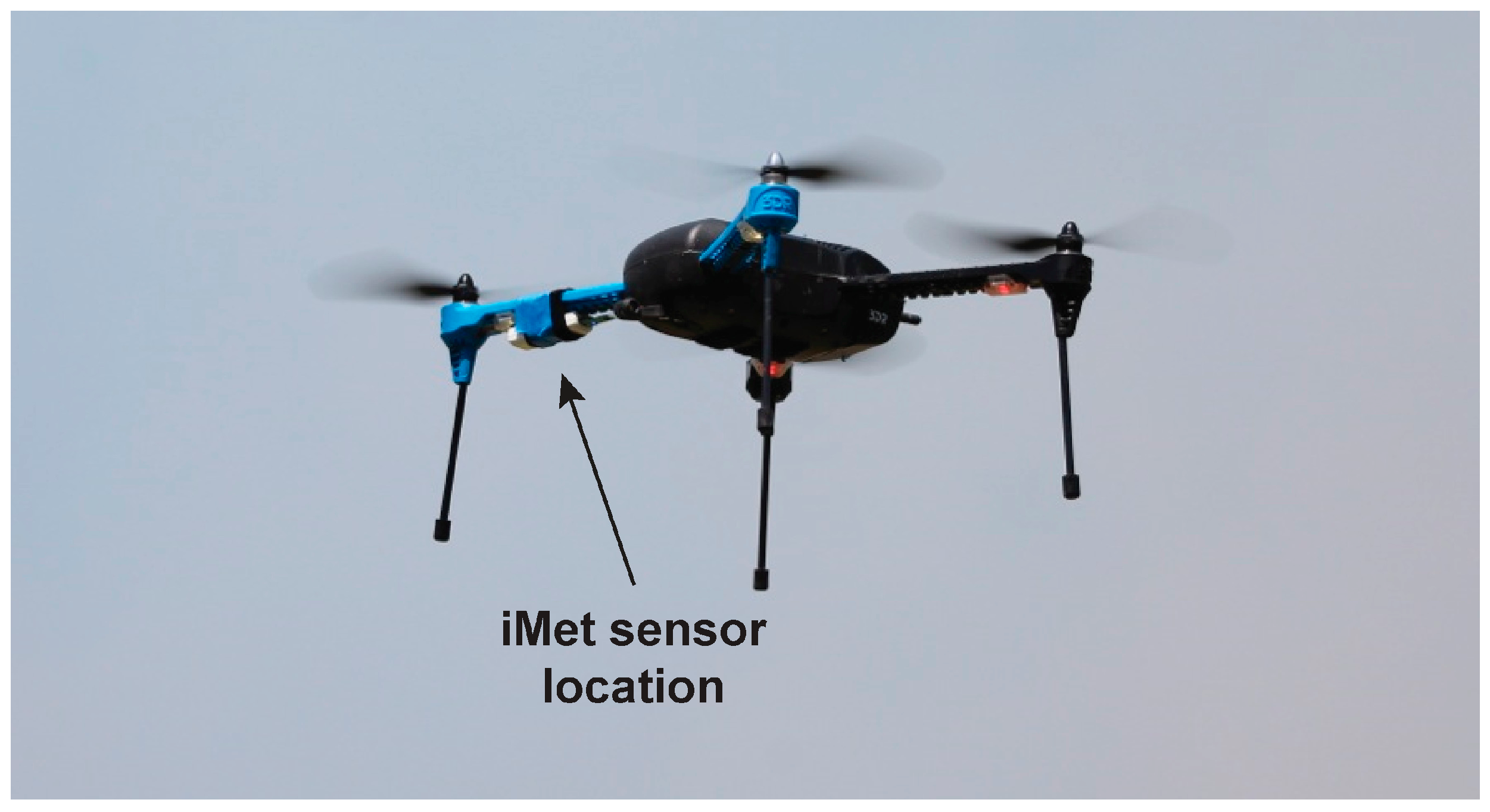
The sUAS platform used for data collection was a 3DR Iris+ (3D Robotics, Inc., Berkeley, CA, USA) multirotor aircraft (Figure 2). The Iris+ weighs 1282 g and is 550 mm in diameter from rotor tip-to-tip. It has a payload of 400 g, and the lithium polymer battery provides up to 22 min of flight time under favorable conditions. The Iris+ sUAS is controlled by an onboard autopilot and is capable of autonomous flight through control via a ground control station through radio frequency communication at 915 MHz.
3.2.2. Sensors
The iMet XQ sensor (International Met Systems, Grand Rapids, MI, USA) was used to collect atmospheric measurements. It is a self-contained unit with temperature, humidity, and pressure sensors as well as a GPS receiver. Weighing 15 g, it has a 120-min battery life and a 16-megabyte storage capacity. The sampling rate is 1–3 Hz. The temperature sensor is of the bead thermistor type with a response time of 2 s. It has an accuracy of ±0.3 °C and a resolution of 0.01 °C. The humidity sensor is the capacitive type with a 5-s response time. It has an accuracy of ±5% relative humidity, and a resolution of 0.07%. The sensor was mounted underneath the rotor arm of the platform and placed near the body of the aircraft to minimize the effects of rotor downwash (Figure 2).
3.3. Surface Weather Observations
Observations from nearby ground weather stations that are part of the Oklahoma Mesonet were used in the analysis to document meteorological conditions at the time of the sUAS flights and provide surface weather observations to supplement the sUAS-derived data. The Oklahoma Mesonet consists of 121 weather stations distributed across the state, with at least one station in every county. The stations consist of a 10 m-tall tower with various sensors that measure more than 20 environmental variables including temperature, relative humidity, pressure, and wind speed [6]. The two Mesonet sites used in this analysis are the Marena site, which is located 11.3 km (7 miles north) of Coyle, OK (36°3′51′′ N, 97°12′45′′ W) and corresponds to the location of the June 29 data collection event; and the Stillwater site, located 2 miles west of Stillwater, OK (36°7′15′′ N, 97°5′42′′ W), which corresponds to the June 30 data collection event.
3.4. Variograms
3.4.1. Sample Variograms
Variogram analysis was completed using the gstat package [27] for the R statistical computing language [28]. Only measurements from the ascent of each profile were used in the analysis, since averaging data from both ascent and descent would skew variations due to a larger time difference, hence variation, from the measurements at lower altitudes. Also, it has been shown that during descent, rotor downwash may introduce updrafts that would impact measurements due to the placement of the sensor on the aircraft [29,30]. As boundary layer turbulence is highly skewed inherently, no observations were removed prior to analysis. For each dataset, the initial lag distance was set to the average point spacing following [24]; however, this resulted in a sparse sample variogram that did not fully represent the structure of the data. Therefore, lag distances were set to one-half the average point spacing, and maximum lag distances were capped at one-half of the sampling extent (maximum above ground altitude) following [26]. However, these suggested parameterizations are based on terrestrial data, which does not exhibit the same scales of variability as atmospheric data. The classical view of high Reynolds number boundary layers, such as the ABL, is that the turbulent flow field can be considered as the superposition of eddies varying in size. The largest eddies would scale with the boundary layer thickness (~1 km) while the smallest are inversely related to the Reynolds number. Here, turbulent energy is supplied from the largest scale motion, and that energy “cascades” down to smaller and smaller eddies until the eddies become sufficiently small that viscosity dissipates the turbulent energy.
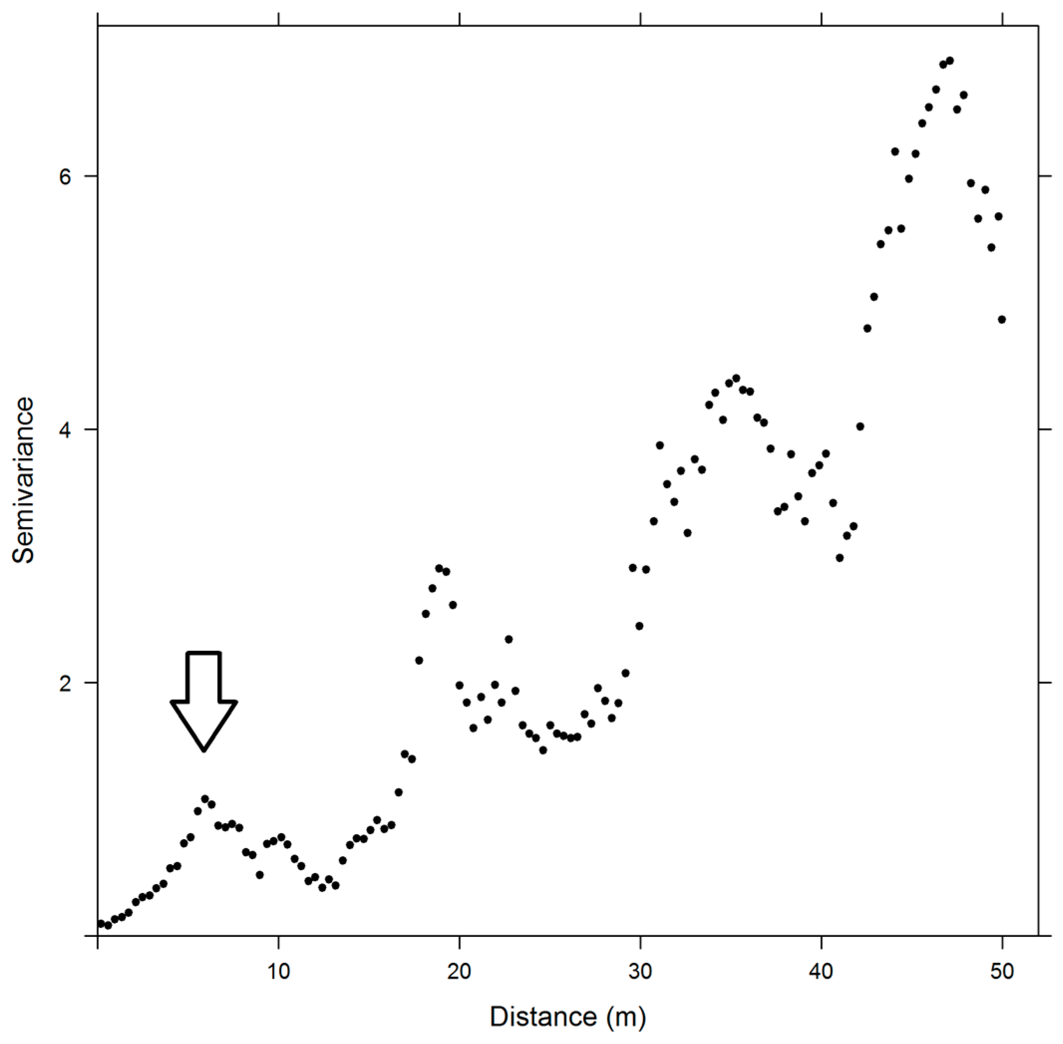
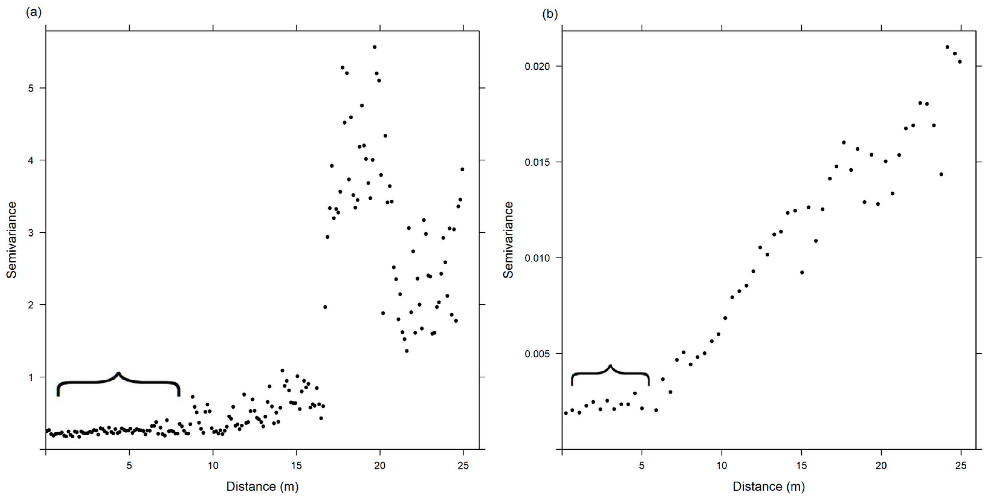
Variograms carry information about all of these scales. In fact, the autocorrelation is commonly used to determine the largest turbulent scales (integral scale) as well as the Taylor microscale. The integral scale is determined from integration of the autocorrelation, and the Taylor microscale (an intermediate-length scale at which turbulent motions are significantly impacted by viscosity) is related to the shape of the autocorrelation near zero lag. Since variograms are a modified form of an autocorrelation function, they carry information about these turbulent structures. Given this information, we expect there to be a certain degree of spatial autocorrelation for all atmospheric samples within the ABL (i.e., we do not expect to see the typical plateau structure of the sample variogram [as shown in Figure 1] until the sampling extent extends beyond the ABL, which could be in the order of 1 km or more). Thus, instead of a single plateau indicating the range of spatial autocorrelation as is typical for terrestrial measurements, we expect the absolute semivariance will exhibit multiple peaks corresponding to the various scales of dominant turbulent structures within the ABL (Figure 3). Since we are interested in identifying the finest spatial scale needed to capture the structure of atmospheric measurements in vertical profiles, our goal is to identify the lag distance where the semivariance first peaks, which is expected to correspond to the finest scale domain, and use this as the maximum lag distance for semivariogram modeling (Figure 3). Other studies have noted similar structures in vertical samples of geological measurements and refer to this phenomena as the hole or periodicity effect [24].
3.4.2. Fitting Model Variograms
Noise and limited sample size can result in some fluctuations within the semivariance estimates, even within each scale domain (Figure 3). Consequently, the data are typically modeled to mitigate the influence of scatter in the variogram and accurately identify the range, sill, and nugget [26]. There are many commonly used model variograms including Gaussian, spherical, and exponential; and proper model selection depends on the spatial continuity of the variable [24]. The chosen model variogram is often eventually used to select ideal weights for further geostatistical analyses, such as kriging [24,25,26], and selecting an incorrect model at this stage can adversely affect the accuracy of subsequent estimates.
Most often, visual inspection is performed on the sample variogram to select the most appropriate model. The sample variograms most closely matched a Gaussian variogram model, and Gaussian models typically work well when there is a small nugget and the curve appears smooth [25]. Following visual assessment, Gaussian model variograms were fitted to all sample variograms.
The Gaussian model is defined as:
where h is the lag and a is the sill. Models were fitted in gstat by minimizing least squares using the Levenberg–Marquardt algorithm [27].
3.4.3. Monin–Obukhov Length Scale Calculations
The Monin–Obukhov length scale
is widely used within micrometeorology to characterize the ABL. It represents a nominal height at which the turbulent production from wind shear is comparable to that from buoyancy. Here, ρ is the density of air at temperature T, Cp is the specific heat capacity at constant pressure, uτ is the friction velocity, κ is the von Kármán constant, and H is the sensible heat flux. Like most ABL measurements, the current study lacks accurate measurements of uτ and H. However, our work follows the work of Dyer [31] and Essa [32] to estimate L given nearby measurements of the surface gradients of wind speed and temperature. Measurements from either the Marena (June 29) or Stillwater (June 30) Mesonet sites were used to record temperature (1.5 m and 9 m above ground), wind speed (2 m and 9 m above ground), and local pressure. These measurements were used to determine potential temperatures (θ1 and θ2), potential temperature difference (Δθ), and wind speed differences (Δu = u2 − u1), which were then used to estimate the gradient Richardson number:
where g is gravitational acceleration and Δz is the difference in heights in the AGL (above ground altitudes) where measurements are acquired. Then, following Businger et al. [33]
where , is the geometric mean height of the measurements used in Ri, φm is an assumed universal function for momentum, and φh is an assumed universal function for heat exchange. The universality of these functions is debated, but for the current work they were estimated using constants from Dyer [31],
allowing for an iterative process to solve for ζ, which provides an estimate for L. The functional forms of the universal function as well as the constant values are questionable, but even under ideal conditions their accuracy within the Monin–Obukhov similarity theory is only 10–20% [34]. Estimating the Monin–Obukhov scale length (L) provides information about the boundary layer stability and the dominant mechanism responsible for turbulent production at the measurement location, which suggests it would be a useful measure for scaling the current measurements.
4. Results
4.1. Flight Summaries
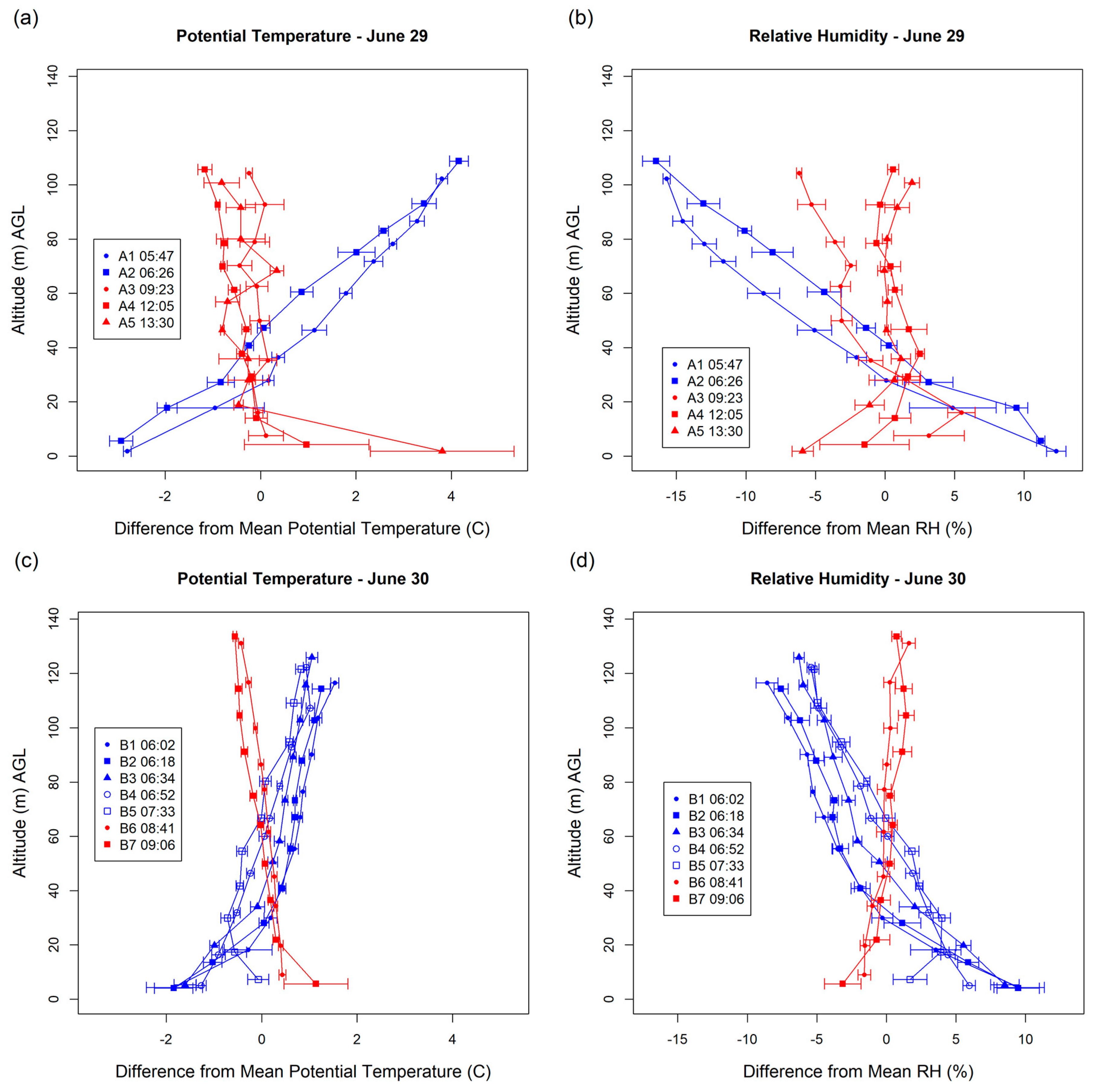
Summary statistics for the 12 flights show similar flight conditions within and between the two flight dates (Table 1). Flights occurred during early morning (pre-sunrise) and late morning/early afternoon to capture temperature inversions from radiative heating during the early part of the day. Each flight lasted between 3 min and 5 min and reached maximum above ground altitudes (AGL) between 100 m and 120 m. On average, 240 measurements were collected for each variable during each flight. Ascents averaged speeds of 1.96 m/s, resulting in an average point spacing of 0.55 points per meter. Mean temperatures ranged from 21.0 °C to 30.6 °C, and mean relative humidity (RH) measurements ranged from 54.7% to 64.3%. Plots of potential temperature and RH for each flight show the profile inversions over the course of each day (Figure 4). Data have been grouped into bins for display purposes, with bin sizes determined by dividing the range of altitude measurements for each flight into deciles. Mean temperature and RH values for each bin were differenced from the overall mean and plotted against the mean altitude of each bin. Standard deviations for each bin are plotted as error bars.
The two earliest flights on June 29 (A1 and A2) show gradually increasing potential temperature and decreasing RH as altitude increases (blue plots in Figure 4a,b). For the later flights (red plots), potential temperature and RH are more homogenous across altitude with slight inversions occurring for RH between the surface and 40 m. For the later flights, both variables exhibit relative stability above 40 m, indicative of a classic stable boundary layer [1]. The homogeneity in temperature and RH above 40 m results from the atmospheric mixing that occurs as the sun warms the Earth and heat begins to radiate upward. The same general trends were observed the following day with flights occurring prior to 08:00 showing an increasing (Temp) or decreasing (RH) relationship with altitude, while flights occurring after 08:00 show less variability and do not exhibit inversions (Figure 4c,d). Overall, there was greater variability in the observations captured on June 29 compared to June 30, both in terms of the overall spread of measurements in the profile as well as the standard deviations for each bin.
4.2. Variogram Modeling
Semivariances were computed for each pair of samples satisfying the maximum lag distance (distance between samples), and Gaussian semivariogram models were fit to the sample points (Figure 5). Two examples (Figure 5) illustrate how the Gaussian model plateaus at the range distance where the sample measurements are no longer spatially autocorrelated within the first scale domain (as determined by the maximum lag distance). The temperature data (Figure 5a) show the nugget being located at approximately 0.015 on the semivariance (y) axis, the sill being located at approximately 0.09, and the range being located at approximately 6 m on the distance (x) axis. The RH data for the same flight show a similar structure, but the semivariance values for the nugget and sill are much higher while the lag distance for the range is only about 3 m. Despite their differences, it is clear from these plots where the semivariance plateaus or levels off, indicating the range distance at which the spatially autocorrelated structure of the data can be captured.
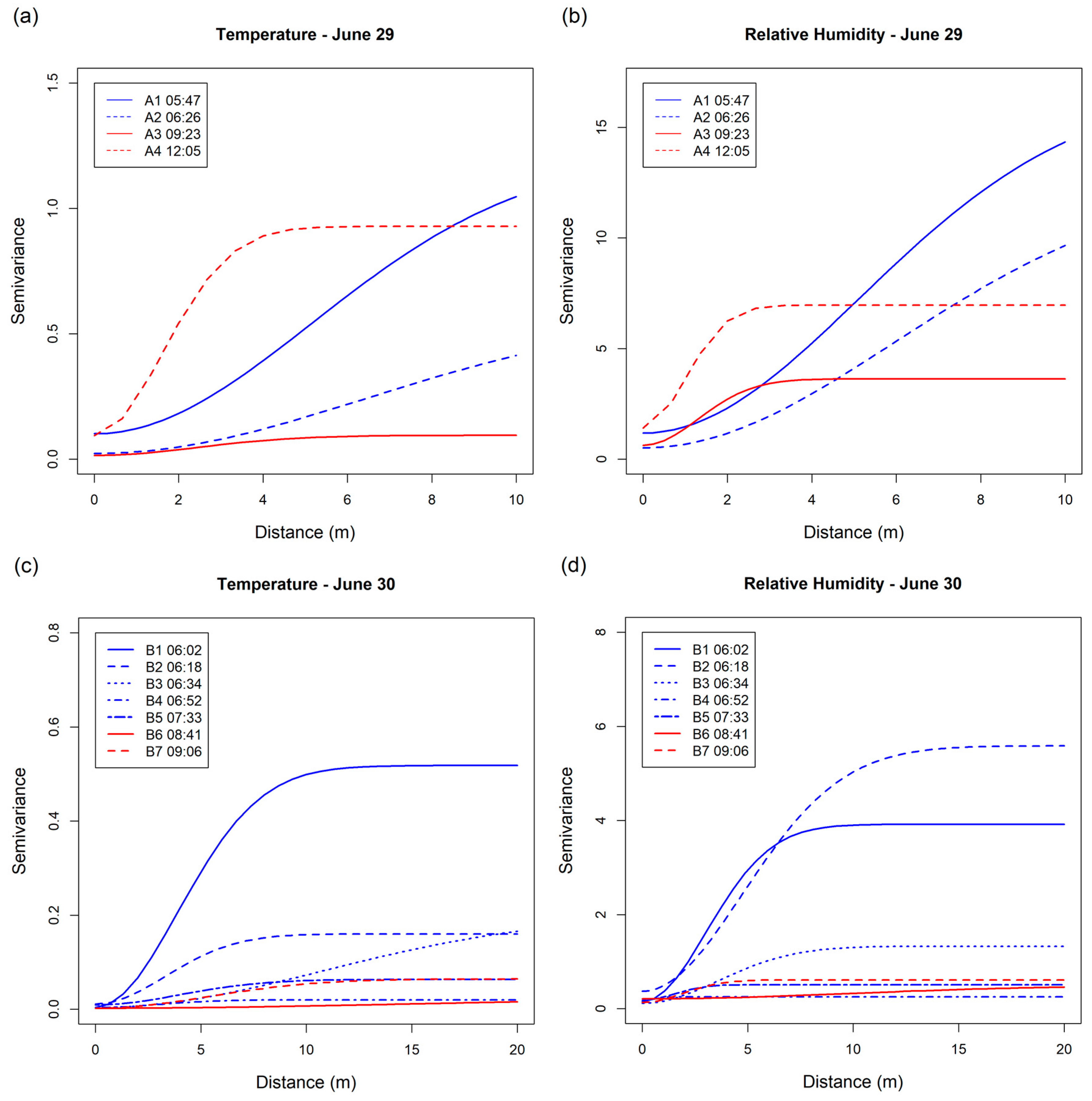
The variogram models for the remaining flights exhibited similar spatial structures to those in Figure 5 but with varying values for nuggets, sills, and ranges. Table 2 presents the computed results while Figure 6 shows the actual model variograms. In general, nugget values did not vary much between the two days for either temperature or RH. Nugget values ranged from 0.002 to 0.101 for temperature and were slightly higher for RH, ranging from 0.111 to 1.402. Small nugget values indicate that at very small sampling lag distances (0.5 m) there is not much variation between measurements. Large nugget values are common for terrestrial, geographic phenomena (e.g., geology), where there can be large differences in a measured variable such as mineral content at small distances (e.g., gold nuggets). Large nuggets (e.g., >½ the sill) are not expected when capturing atmospheric data and were not observed during this sampling campaign.
Sill values for temperature also showed little variability across both days, ranging between 0.095 and 1.214 on June 29 and between 0.020 and 0.518 on June 30. Sill values for RH were more variable, ranging from 3.627 to 12.594 on June 29 and from 0.248 to 3.920 on June 30. For both temperature and RH, there was greater variation in sill position for the June 29 flights compared to the June 30 flights. The sill value quantifies the maximum semivariance at the range distance identified by the variogram model (Figure 3). Larger sill values indicate larger variances between samples at the distance where spatial autocorrelation begins to plateau. In general, sills were larger for both variables on both days for the early morning flights compared to the later flights because the atmosphere had not mixed at that point, so there is greater variance in measurements between lag distances.
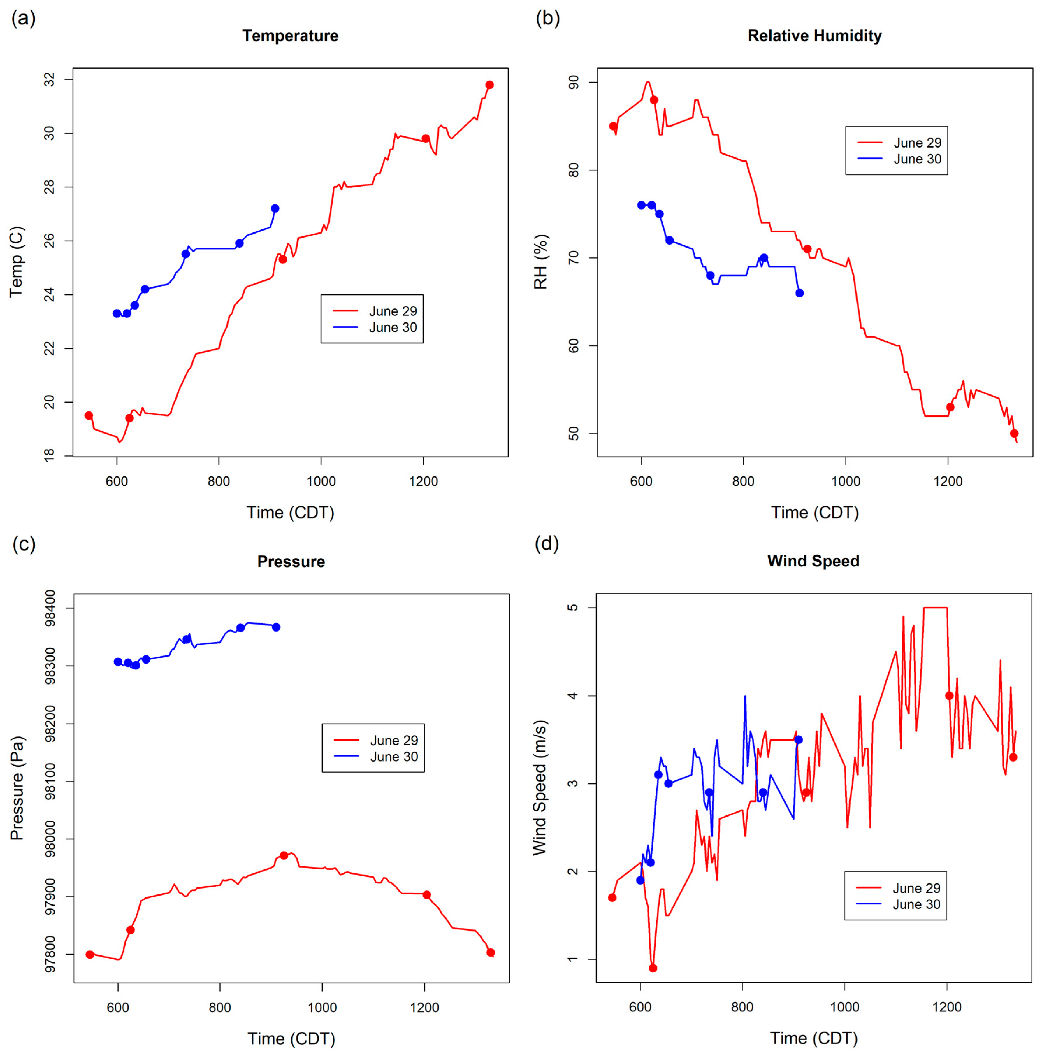
It should be noted that the sills for RH on June 29 were several times larger than those captured on June 30. These differences may be due to the more variable weather conditions on June 30 as observed from the Mesonet towers (Figure 7). In particular, wind speeds were greater on the morning of June 30 indicating increased frictional mixing within the lower portion of the boundary layer (100–150 m). As seen in the profile plots (Figure 4), the range of RH values is much greater on June 29 compared to June 30, and the maximum altitude of the June 29 flights is about 20–30 m less than June 30 (Table 1). Together, these results indicate the atmosphere was likely less mixed, and therefore more variable, during the morning flights on June 29 compared to June 30. As a result, the RH measurements at each distance lag were more dissimilar on June 29 than they were on June 30, manifesting in greater sill values.
Range values show several interesting trends (Figure 6). On June 29, the ranges for temperature and RH are quite similar across each flight, with larger ranges computed for the early morning flights and comparably smaller ranges for the later flights. For the June 30 flights, with the exception of Flight B6, and an outlying value for temperature during Flight B3, range values were relatively stable, ranging from about 2–5 m. These results indicate that during the early morning when the lower atmosphere is not yet mixed, samples can be collected at larger lag distances while still capturing the spatial structure of the profile. Meanwhile, when the atmosphere is mixed, particularly during later times of the day, more frequent sampling is needed to capture changes in the vertical profile. These findings are consistent with the expectation that the ABL is at a lower Reynolds number in the morning when it is forming, which results in the finest scales being larger (i.e., smallest turbulent length scales are inversely related to the Reynolds number). Thus, fewer measurements spaced further apart are needed to capture the structure of the atmosphere before the Earth’s surface warms and mixing occurs.
Lastly, the computed Monin–Obukhov length scales (L) (Table 2) show that there does appear to be some correlation with scatter as L increases between the ranges for both temperature and relative humidity. Given the uncertainty in L and relatively small sample size, the current results were not scaled with L, but further investigation with a larger sample size is needed.
Standardized variograms allow for comparison of range values irrespective of the varying sill values, which can aid in interpretation. Variograms were standardized to a semivariance of one by plotting the semivariance minus the nugget divided by the partial sill (sill-nugget) against the lag distance (Figure 8). For the June 29 flights, there is a clear distinction between the early morning (red lines) and late morning/early afternoon flights (blue lines). Range values in the late morning are smaller than those in the early morning, again suggesting that more frequent sampling is needed to capture the atmospheric profile prior to mixing. On June 30, where there was less change in the atmosphere between the early-morning and late-morning/early-afternoon flights, there is less distinction in range values. Values were relatively stable across all flights, although range values appear to decrease slightly as the morning progresses. Flights B3 and B6 also appear as outliers, particularly in the temperature plot (Figure 8c).
5. Discussion
While turbulent flow fields such as an ABL obey governing equations, their signals are not repeatable, which forces the results to be reported as statistics for comparison. Spatial autocorrelation functions provide fundamental insights about the size and distribution of coherent structures within a turbulent flow (e.g., [35,36,37]). Variograms generated for atmospheric measurements in the ABL capture the distribution of scales via multiple peaks or plateaus at which autocorrelation dissipates over a range of length scales, with the smallest structures having the highest correlation (i.e., smallest semivariance). Thus, the largest sample separation distance that can still capture the smallest scale structures should be related to the range observed for the first peak/plateau from the semivariance plot (Figure 3). Following this assumption, we found that optimal sampling scales for vertical measurements of temperature taken from sUAS were about 5 m for early morning flights prior to atmospheric mixing. Once mixing had occurred, more frequent sampling was needed (~3 m) to capture the data structure. If researchers are unsure of the status of the atmosphere at the time of data collection, we recommend using smaller sampling distances to ensure that small scale structures are not missed. The optimal sampling scales for RH were slightly smaller than those for temperature, with range values of approximately 1.5–2 m after mixing had occurred. Again, these scales were found to be sufficient for capturing the first scale domain for temperature and RH within the lower portion of the ABL for this study; further research is needed to identify the periodicity of additional scale domains within the ABL. Additionally, researchers looking to capture micro fluctuations may require smaller sampling scales.
Flight A5 could not be modeled with a semivariogram and, therefore, results were not reported or included in our analysis. The likely reason that A5 could not be modeled is because as the process of boundary layer mixing unfolds, the portion of the atmosphere in direct contact with the Earth becomes homogenized. With homogenization, the first scale domain becomes ever smaller and eventually is undetectable in the sample variogram. This phenomenon is known as the pure nugget effect [24], and makes model fitting difficult because there is no identifiable plateau within the maximum lag distance (Figure 9). While the absence of a peak/plateau within the maximum lag distance signals that the first scale domain is located at a larger scale, it does not change the minimum sampling scales that should be used in the absence of knowledge about the structure of the atmosphere. For Flight B6, which exhibited a similar pattern (Figure 9b), even though a variogram could be fitted to the data, the associated range distances for temperature (19.934) and RH (13.597) are likely more representative of the second scale domain. While we were limited in the altitudes we could fly for these missions, we intend to profile the entire ABL (up to 1000 m) in future campaigns in order to identify the full set of scale domains and inform future data collection via sUAS.
Several limitations of this study should be noted. First, our findings are based on a relatively small sample size in an effort to control for seasonality and geographic location as well as platform and sensor calibration. The flights described in this paper were performed on consecutive days with similar weather patterns in locations near Oklahoma Mesonet sites in order to validate the sensors used in the study. We were limited to flying at altitudes of no more than 304 m (1000 ft) above ground, so in this study we were unable to capture the entire profile of the ABL. However, in future campaigns and with adequate permissions, we aim to survey the entire ABL. Additionally, UAS flights are currently limited to daylight hours, so our analyses do not capture diurnal differences in profile structure. In terms of location, these flights represent atmospheric conditions in a primarily rural area, and atmospheric structures in urban areas are likely to vary. Our samples were captured under relatively normal atmospheric conditions in order to determine baseline standards for vertical sampling from sUAS. Next steps will also include capturing comparable measurements during atmospheric events such as storm formation. Lastly, we limited our analysis to vertical sampling events, and our next steps will include characterizing both the vertical and horizontal dimensions simultaneously to begin determining the optimal horizontal scales to measure changing atmospheric phenomena.
6. Conclusions
This study used variogram modeling, a common geostatistical technique in the geographical sciences, to determine vertical spatial sampling scales for two atmospheric variables (temperature and relative humidity) captured from a small, unmanned aircraft system (sUAS). The key findings from our analysis show that variogram modeling can serve as a useful methodology for identifying the finest scale domain of atmospheric vertical profiles. Future work will focus on capturing the entire extent of the ABL, as well as integrating optimal spatial sampling scales in the horizontal direction with those in the vertical dimension, as a basis for collecting measurements from sUAS.
Acknowledgments
This research is supported by a grant from the U.S. National Science Foundation (NSF) [IIA-1539070] “RII Track-2 FEC: Unmanned Aircraft Systems for Atmospheric Physics”. The authors would like to thank Taylor Mitchell, Jordan Feight, and Geoffrey Donnell from Oklahoma State University and Dr. Phil Chilson from the University of Oklahoma for helping with data collection and useful discussions.
Author Contributions
B.H. and A.F. conceived of and designed the experiments. J.J. managed field data collection. B.H. contributed to data analysis and interpretation. All authors contributed to writing the paper.
Conflicts of Interest
There are no conflicts of interest to disclose.
References
- Stull, R.B. An Introduction to Boundary Layer Meteorology, 1st ed.; Kluwer Academic Publishers: Dordrecht, The Netherlands, 1988. [Google Scholar]
- Garratt, J.R. The Atmospheric Boundary Layer, 1st ed.; Cambridge University Press: Cambridge, New York, NY, USA, 1994. [Google Scholar]
- Mayer, S.; Sandvik, A.; Jonassen, M. O.; Reuder, J. Atmospheric profiling with the UAS SUMO: A new perspective for the evaluation of fine-scale atmospheric models. Meteorol. Atmos. Phys. 2012, 116, 15–26. [Google Scholar] [CrossRef]
- LaDue, D.S.; Heinselman, P.L.; Newman, J.F. Strengths and limitations of current radar systems for two stakeholder groups in the southern plains. Bull. Am. Meteorol. Soc. 2010, 91, 899–910. [Google Scholar] [CrossRef]
- Frew, E.W.; Elston, J.; Argrow, B.; Houston, A.; Rasmussen, E. Sampling severe local storms and related phenomena: Using unmanned aircraft systems. IEEE Robot. Autom. Mag. 2012, 19, 85–95. [Google Scholar] [CrossRef]
- McPherson, R.A.; Fiebrich, C.A.; Crawford, K. C.; Kilby, J.R.; Grimsley, D.L.; Martinez, J.E.; Basara, J.B.; Illston, B.G.; Morris, D.A.; Kloesel, K.A. Statewide monitoring of the mesoscale environment: A technical update on the Oklahoma Mesonet. J. Atmos. Ocean. Tech. 2007, 24, 301–321. [Google Scholar] [CrossRef]
- Fujita, T.T. A Review of Researches on Analytical Mesometeorology; Mesometeorology Project: Department of the Geophysical Sciences, University of Chicago, Chicago, IL, USA, 1962. [Google Scholar]
- Hill, M.; Konrad, T.; Meyer, J.; Rowland, J. A small, radio-controlled aircraft as a platform for meteorological sensors. Appl. Phys. Lab. Tech. Digest 1970, 10, 11–19. [Google Scholar]
- Jensen, J.R. Introductory Digital Image Processing: A Remote Sensing Perspective; Prentice Hall, Inc.: Old Tappan, NJ, USA, 1986. [Google Scholar]
- Doviak, R.J.; Zrnic, D.S. Doppler Radar & Weather Observations; Academic Press: Cambridge, MA, USA, 2014. [Google Scholar]
- Bendix, J.; Fries, A.; Zárate, J.; Trachte, K.; Rollenbeck, R.; Pucha-Cofrep, F.; Paladines, R.; Palacios, I.; Orellana, J.; Oñate-Valdivieso, F. RadarNet-Sur First Weather Radar Network In Tropical High Mountains. Bull. Am. Meteorol. Soc. 2017, 98, 1235–1254. [Google Scholar] [CrossRef]
- RoyChowdhury, A.; Sheldon, D.; Maji, S.; Learned-Miller, E. Distinguishing Weather Phenomena from Bird Migration Patterns in Radar Imagery. In Proceedings of the 2016 IEEE Conference on Computer Vision and Pattern Recognition Workshops (CVPRW), Las Vegas, NV, USA, 26 June–1 July 2016; pp. 10–17. [Google Scholar]
- Farnsworth, A.; Van Doren, B.M.; Hochachka, W.M.; Sheldon, D.; Winner, K.; Irvine, J.; Geevarghese, J.; Kelling, S. A characterization of autumn nocturnal migration detected by weather surveillance radars in the northeastern USA. Ecol. Appl. 2016, 26, 752–770. [Google Scholar] [CrossRef] [PubMed]
- Golbon-Haghighi, M.-H.; Zhang, G.; Li, Y.; Doviak, R.J. Detection of Ground Clutter from Weather Radar Using a Dual-Polarization and Dual-Scan Method. Atmosphere 2016, 7, 83. [Google Scholar] [CrossRef]
- Frazier, A.E.; Mathews, A.J.; Hemingway, B.; Crick, C.; Martin, E.; Smith, S.W. Integrating unmanned aircraft systems (UAS) into GIScience: Challenges and opportunities. Conference Presentation, GI_Forum, Salzburg, Austria, 3–6 July 2017. [Google Scholar]
- Federal Aviation Administration. Part 107 of the Small Unmanned Aircraft Regulations. Available online: https://www.faa.gov/news/fact_sheets/news_story.cfm?newsId=20516 (assessed on 19 March 2017).
- Elston, J.; Argrow, B.; Stachura, M.; Weibel, D.; Lawrence, D.; Pope, D. Overview of small fixed-wing unmanned aircraft for meteorological sampling. J. Atmos. Ocean. Tech. 2015, 32, 97–115. [Google Scholar] [CrossRef]
- Houston, A.L.; Argrow, B.; Elston, J.; Lahowetz, J.; Frew, E.W.; Kennedy, P.C. The collaborative Colorado–Nebraska unmanned aircraft system experiment. Bull. Am. Meteorol. Soc. 2012, 93, 39–54. [Google Scholar] [CrossRef]
- Roadman, J.; Elston, J.; Argrow, B.; Frew, E. Mission Performance of the Tempest Unmanned Aircraft System in Supercell Storms. J. Aircraft. 2012, 49, 1821–1830. [Google Scholar] [CrossRef]
- Cook, D.; Strong, P.; Garrett, S.; Marshall, R. A small unmanned aerial system (UAS) for coastal atmospheric research: Preliminary results from New Zealand. J. R. Soc. N. Z. 2013, 43, 108–115. [Google Scholar] [CrossRef]
- Cassano, J.J. Observations of atmospheric boundary layer temperature profiles with a small unmanned aerial vehicle. Antarct. Sci. 2014, 26, 205–213. [Google Scholar] [CrossRef]
- Bolstad, P. GIS Fundamentals: A First Text on Geographic Information Systems, 2nd ed.; Eider Press: White Bear lake, MN, USA, 2005. [Google Scholar]
- Crick, C.; Pfeffer, A. Loopy belief propagation as a basis for communication in sensor networks. In UAI’03, Proceedings of the Nineteenth Conference on Uncertainty in Artificial Intelligence; Morgan Kaufmann Publishers Inc.: San Francisco, CA, USA, 2003; pp. 159–166. [Google Scholar]
- Isaaks, E.H.; Srivastava, R.M. Applied Geostatistics; Oxford University Press: England, UK, 1989. [Google Scholar]
- Burrough, P.A.; McDonnell, R.; McDonnell, R.A.; Lloyd, C.D. Principles of Geographical Information Systems; Oxford University Press: England, UK, 2015. [Google Scholar]
- Oliver, M.A.; Webster, R. Basic Steps in Geostatistics: The Variogram and Kriging; Springer: New York, NY, USA, 2015. [Google Scholar]
- Pebesma, E.J. Multivariable geostatistics in S: The gstat package. Comput. Geosci. 2004, 30, 683–691. [Google Scholar]
- R Core Team. R: A Language and Environment for Statistical Computing. Available online: https://www.r-project.org/ (accessed on 19 March 2017).
- Chilson, P.; Huck, R.; Fiebrich, C.; Cornish, D.; Wawrzyniak, T.; Mazuera, S.; Dixon, A.; Burns, E.; Greene, B. Calibration and Validation of Weather Sensors for Rotary-Wing UAS: The Devil is in the Details. In Proceedings of the 97th American Meteorological Society Annual Meeting, Seattle, WA, USA, 21 January 2017. [Google Scholar]
- Jacob, J.; Axisa, D.; Oncley, S. Unmanned Aerial Systems for Atmospheric Research: Instrumentation Isues for Atmospheric Measurements. In Proceedings of the NCAR/EOL Community Workshop for Unmanned Aerial Systems for Atmospheric Research, Boulder, CO, USA, 21–24 February 2017. [Google Scholar]
- Dyer, A. A review of flux-profile relationships. Bound. Layer Meteorol. 1974, 7, 363–372. [Google Scholar] [CrossRef]
- Essa, K.S. Estimation of Monin-Obukhov Length Using RIchardson and Bulk Richardson Number. In Proceedings of the 2nd Conference on Nuclear and Particle Physics, Cairo, Egypt, 13–17 November 1999. [Google Scholar]
- Businger, J. A.; Wyngaard, J.C.; Izumi, Y.; Bradley, E.F. Flux-profile relationships in the atmospheric surface layer. J. Atmos. Sci. 1971, 28, 181–189. [Google Scholar] [CrossRef]
- Foken, T. 50 years of the Monin–Obukhov similarity theory. Bound. Layer Meteorol. 2006, 119, 431–447. [Google Scholar] [CrossRef]
- Yeung, P. Lagrangian investigations of turbulence. Annu. Rev. Fluid Mech. 2002, 34, 115–142. [Google Scholar] [CrossRef]
- Elbing, B.R.; Winkel, E.S.; Ceccio, S.L.; Perlin, M.; Dowling, D.R. High-reynolds-number turbulent-boundary-layer wall-pressure fluctuations with dilute polymer solutions. Phys. Fluids 2010, 22, 085104. [Google Scholar] [CrossRef]
- Horn, G.; Ouwersloot, H.; De Arellano, J.V.-G.; Sikma, M. Cloud Shading Effects on Characteristic Boundary-Layer Length Scales. Bound. Layer Meteorol. 2015, 157, 237–263. [Google Scholar] [CrossRef]
Figure 1.
Example of a typical variogram produced from plotting semivariance versus lag distance. Locations of nugget, range, and sill are shown.
Figure 1.
Example of a typical variogram produced from plotting semivariance versus lag distance. Locations of nugget, range, and sill are shown.
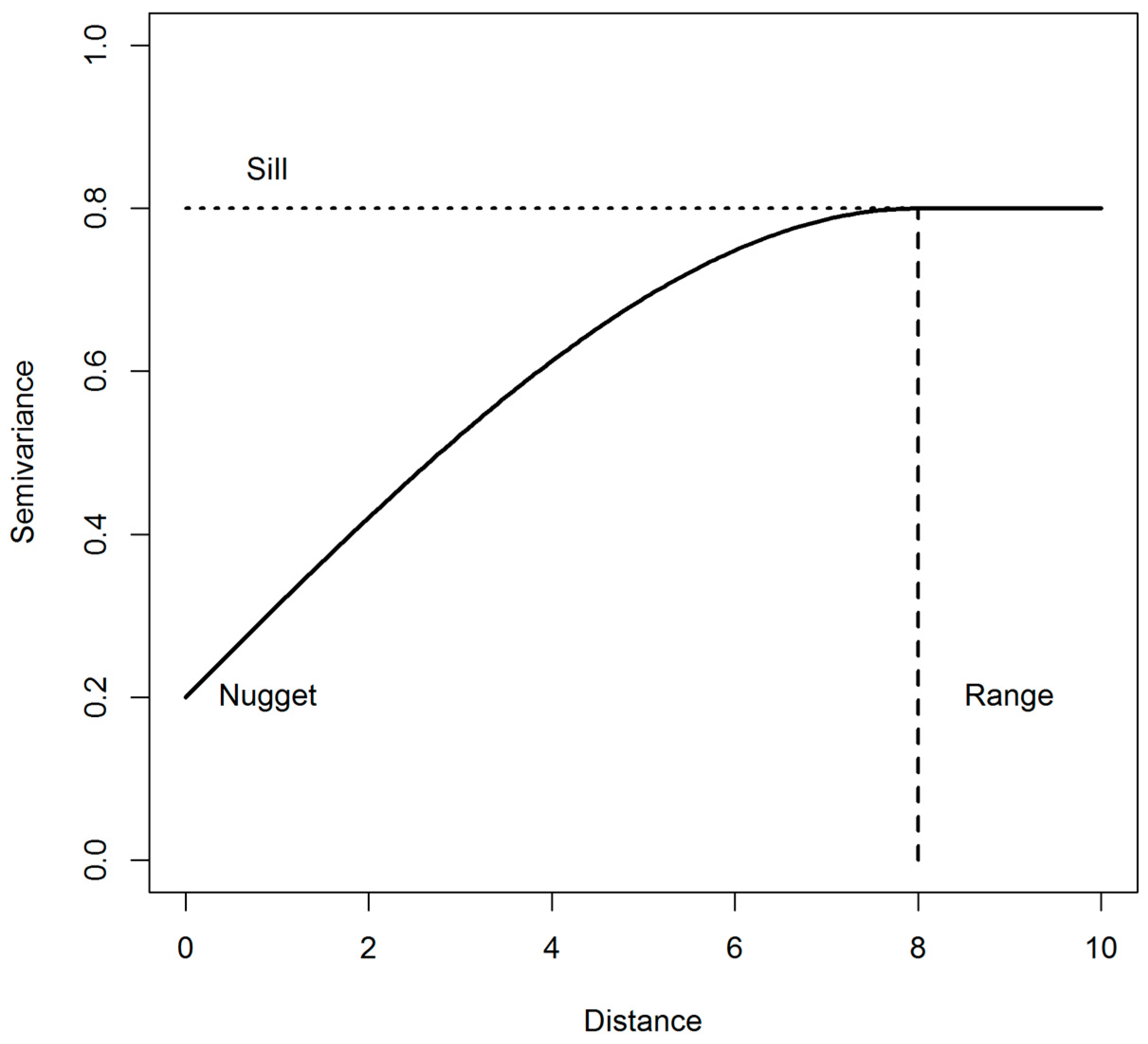
Figure 2.
Location of iMet XQ sensor mounted on underside of 3DR Iris+ multirotor platform.

Figure 3.
Sample variogram displaying increasing scales of variability (scale domains) with distance.
Figure 3.
Sample variogram displaying increasing scales of variability (scale domains) with distance.

Figure 4.
Profile plots for (a) June 29 potential temperature, (b) June 29 relative humidity, (c) June 30 potential temperature, and (d) June 30 relative humidity. Flight start times are in Central Daylight Time (UTC-5).
Figure 4.
Profile plots for (a) June 29 potential temperature, (b) June 29 relative humidity, (c) June 30 potential temperature, and (d) June 30 relative humidity. Flight start times are in Central Daylight Time (UTC-5).

Figure 5.
Sample variograms with Gaussian variogram models fitted to (a) temperature and (b) relative humidity data from flight A3 on June 29.
Figure 5.
Sample variograms with Gaussian variogram models fitted to (a) temperature and (b) relative humidity data from flight A3 on June 29.
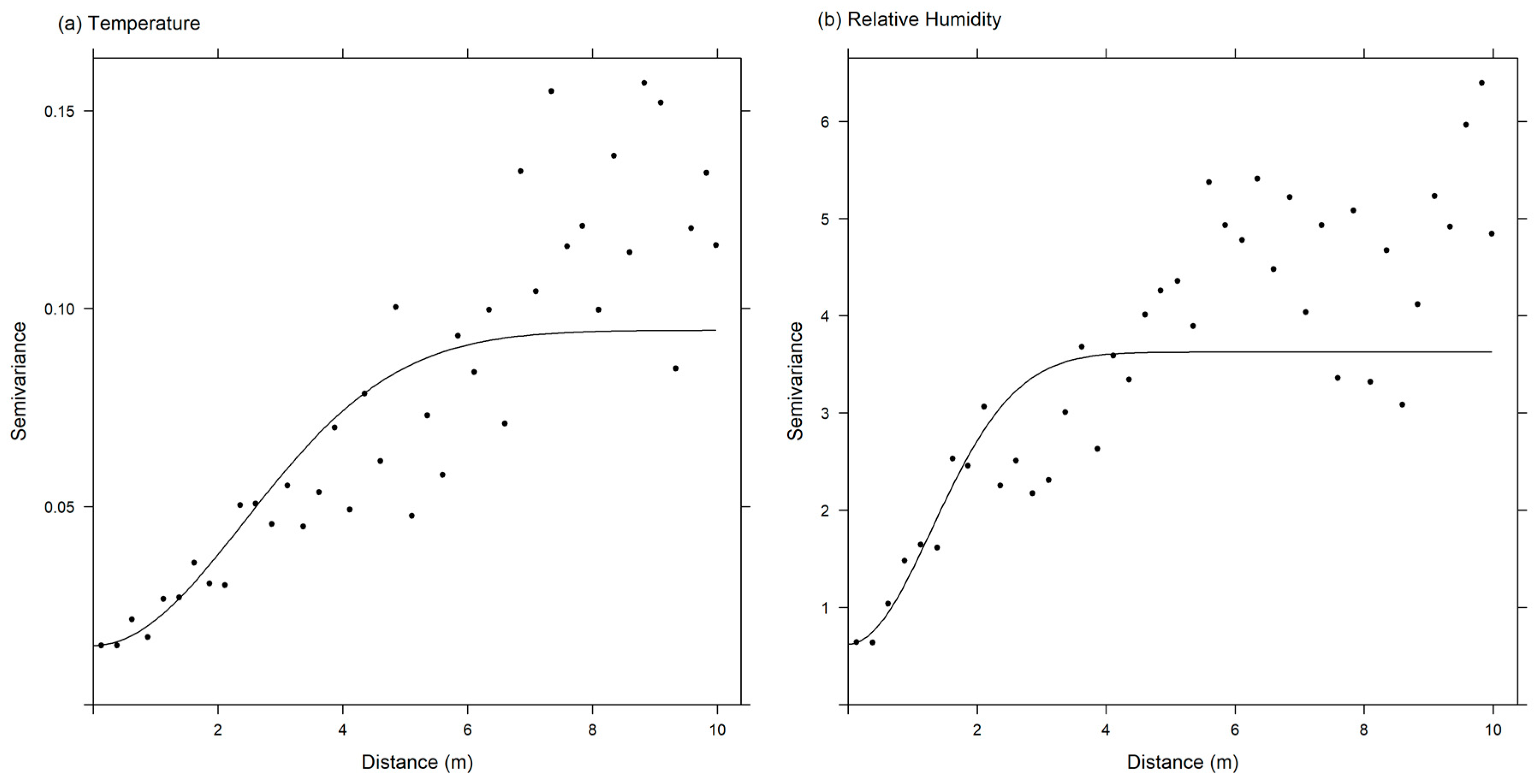
Figure 6.
Fitted Gaussian variogram models for (a) June 29 temperature, (b) June 29 relative humidity, (c) June 30 temperature, and (d) June 30 relative humidity.
Figure 6.
Fitted Gaussian variogram models for (a) June 29 temperature, (b) June 29 relative humidity, (c) June 30 temperature, and (d) June 30 relative humidity.

Figure 7.
Weather conditions at corresponding Mesonet stations for (a) temperature, (b) relative humidity, (c) pressure, and (d) wind speed. Dots indicate start time of each ascent.
Figure 7.
Weather conditions at corresponding Mesonet stations for (a) temperature, (b) relative humidity, (c) pressure, and (d) wind speed. Dots indicate start time of each ascent.

Figure 8.
Standardized variogram models for (a) June 29 temperature, (b) June 29 relative humidity, (c) June 30 temperature, and (d) and June 30 relative humidity.
Figure 8.
Standardized variogram models for (a) June 29 temperature, (b) June 29 relative humidity, (c) June 30 temperature, and (d) and June 30 relative humidity.
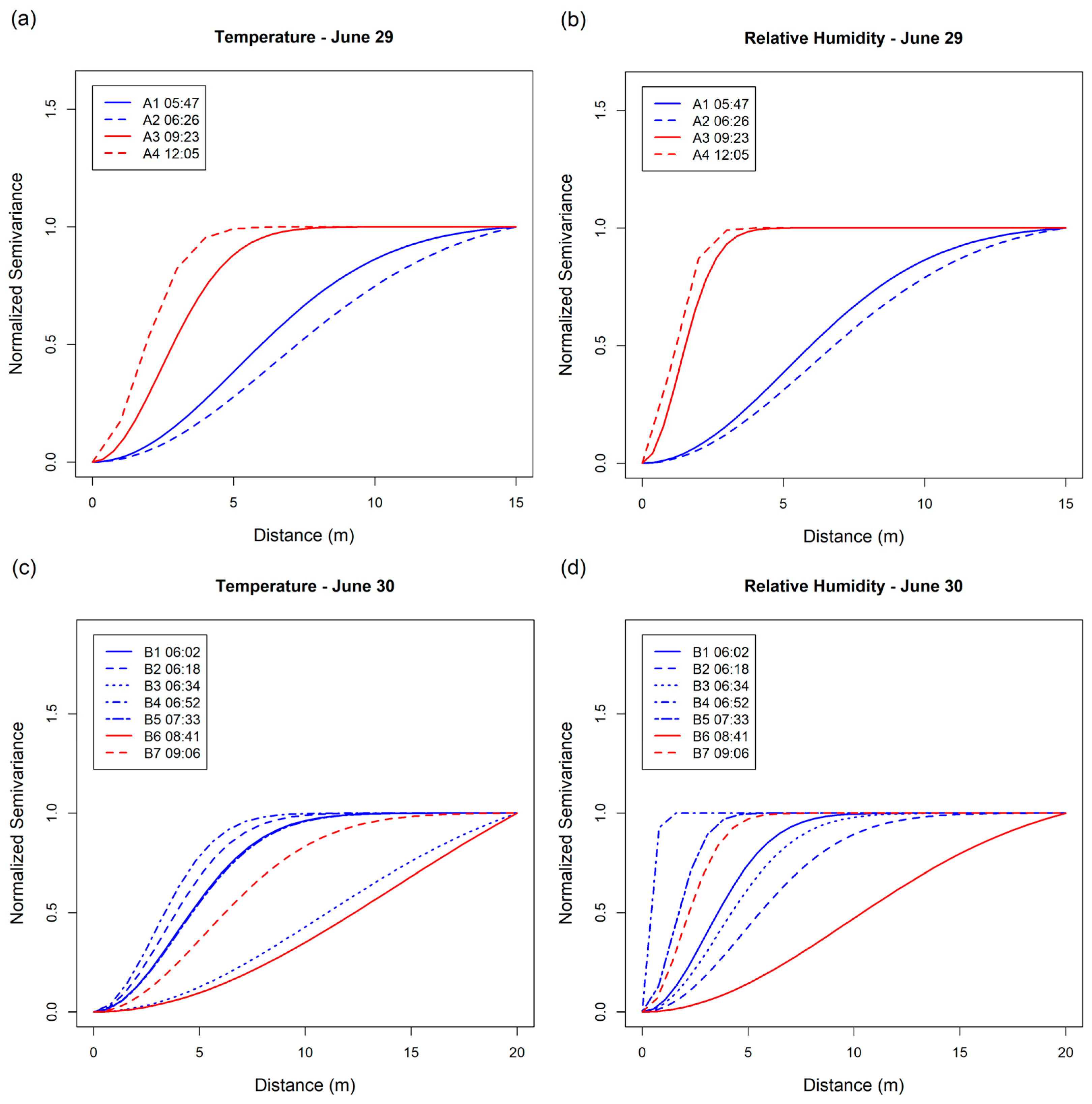
Figure 9.
Sample variograms of flight A5 on June 29 (a) and B6 on June 30 (b).


Table 1.
Flight information and summary statistics. Temperature (Temp) is reported in degrees Celsius and relative humidity (RH) is reported in percentages. Start times note the start of each ascent and end times are the time at which the flight reached its maximum altitude. Flight times are in Central Daylight Time (UTC-5).
| Flight ID | Date | Start Time | End Time | Max Alt. AGL (m) | No. Obs. | Min Temp | Mean Temp | Max Temp | Min RH | Mean RH | Max RH |
|---|---|---|---|---|---|---|---|---|---|---|---|
| A1 | 29-Jun | 5:47:30 | 5:52:06 | 107.87 | 277 | 18.11 | 21.02 | 24.94 | 46.6 | 62.98 | 76.1 |
| A2 | 29-Jun | 6:26:06 | 6:29:41 | 110.95 | 216 | 19.06 | 22.13 | 26.47 | 41.0 | 58.8 | 70.6 |
| A3 | 29-Jun | 9:23:45 | 9:27:23 | 111.21 | 219 | 23.77 | 24.58 | 26.33 | 51.3 | 57.85 | 67.1 |
| A4 | 29-Jun | 12:05:23 | 12:09:55 | 111.39 | 273 | 27.51 | 28.92 | 33.39 | 47.6 | 55.28 | 59.9 |
| A5 | 29-Jun | 13:30:48 | 13:37:42 | 111.97 | 415 | 29.35 | 30.6 | 36.09 | 47.7 | 54.71 | 60.5 |
| B1 | 30-Jun | 6:02:10 | 6:05:56 | 130.06 | 227 | 21.09 | 23.46 | 25.07 | 54.9 | 64.26 | 76.3 |
| B2 | 30-Jun | 6:18:54 | 6:22:22 | 130.48 | 210 | 21.27 | 23.71 | 25.17 | 54.5 | 62.74 | 74.5 |
| B3 | 30-Jun | 6:34:31 | 6:37:59 | 133.30 | 213 | 21.75 | 23.6 | 24.84 | 56 | 63.01 | 72.6 |
| B4 | 30-Jun | 6:52:45 | 6:56:05 | 135.40 | 202 | 22.13 | 23.55 | 24.63 | 56.6 | 62.32 | 69 |
| B5 | 30-Jun | 7:33:31 | 7:38:06 | 132.44 | 278 | 22.64 | 23.52 | 24.55 | 58 | 63.98 | 68.9 |
| B6 | 30-Jun | 8:41:57 | 8:44:32 | 137.10 | 156 | 25.02 | 25.61 | 26.19 | 55.2 | 57.15 | 59.4 |
| B7 | 30-Jun | 9:06:49 | 9:10:00 | 141.99 | 193 | 25.39 | 26.05 | 28.17 | 49.6 | 55.08 | 57.3 |
Table 2.
Variogram results and fit diagnostics (RMSE) for all flights showing sill, range, and nugget values for temperature (Temp) and relative humidity (RH) and estimates of the Monin–Obukhov length scale [L(m)].
Table 2.
Variogram results and fit diagnostics (RMSE) for all flights showing sill, range, and nugget values for temperature (Temp) and relative humidity (RH) and estimates of the Monin–Obukhov length scale [L(m)].
| Flight ID | Temp Sill | Temp Range | Temp Nugget | Temp RMSE | RH Sill | RH Range | RH Nugget | RH RMSE | L (m) |
|---|---|---|---|---|---|---|---|---|---|
| A1 | 1.214 | 7.258 | 0.101 | 0.300 | 16.623 | 7.239 | 1.178 | 1.121 | 69 |
| A2 | 0.584 | 9.150 | 0.022 | 0.031 | 12.594 | 8.410 | 0.509 | 2.065 | 1200 |
| A3 | 0.095 | 3.423 | 0.015 | 0.024 | 3.627 | 1.831 | 0.622 | 1.031 | −3700 |
| A4 | 0.928 | 2.280 | 0.094 | 0.354 | 6.961 | 1.397 | 1.402 | 1.601 | −4300 |
| A5 * | - | - | - | - | - | - | - | - | −4500 |
| B1 | 0.518 | 5.513 | 0.004 | 0.060 | 3.920 | 4.295 | 0.147 | 0.572 | 4500 |
| B2 | 0.160 | 4.676 | 0.011 | 0.058 | 2.364 | 2.511 | 0.362 | 1.979 | 5600 |
| B3 | 0.200 | 15.131 | 0.003 | 0.017 | 1.327 | 5.071 | 0.111 | 0.222 | 4100 |
| B4 | 0.020 | 4.028 | 0.003 | 0.007 | 0.248 | 0.496 | 0.146 | 0.200 | 11000 |
| B5 | 0.063 | 5.592 | 0.009 | 0.014 | 0.508 | 2.058 | 0.174 | 0.078 | −26000 |
| B6 | 0.023 | 19.934 | 0.002 | 0.001 | 0.490 | 13.597 | 0.207 | 0.053 | −7900 |
| B7 | 0.064 | 7.463 | 0.002 | 0.020 | 0.610 | 2.655 | 0.130 | 0.111 | −5400 |
* Variogram model could not be fitted to measurements from flight A5.
© 2017 by the authors. Licensee MDPI, Basel, Switzerland. This article is an open access article distributed under the terms and conditions of the Creative Commons Attribution (CC BY) license (http://creativecommons.org/licenses/by/4.0/).
Share and Cite
MDPI and ACS Style
Hemingway, B.L.; Frazier, A.E.; Elbing, B.R.; Jacob, J.D. Vertical Sampling Scales for Atmospheric Boundary Layer Measurements from Small Unmanned Aircraft Systems (sUAS). Atmosphere 2017, 8, 176. https://doi.org/10.3390/atmos8090176
AMA Style
Hemingway BL, Frazier AE, Elbing BR, Jacob JD. Vertical Sampling Scales for Atmospheric Boundary Layer Measurements from Small Unmanned Aircraft Systems (sUAS). Atmosphere. 2017; 8(9):176. https://doi.org/10.3390/atmos8090176
Chicago/Turabian StyleHemingway, Benjamin L., Amy E. Frazier, Brian R. Elbing, and Jamey D. Jacob. 2017. "Vertical Sampling Scales for Atmospheric Boundary Layer Measurements from Small Unmanned Aircraft Systems (sUAS)" Atmosphere 8, no. 9: 176. https://doi.org/10.3390/atmos8090176
Note that from the first issue of 2016, this journal uses article numbers instead of page numbers. See further details here.