Effects of Unstable Stratification on Ventilation in Hong Kong


1
Insitute of Meteorology and Climatology, Leibniz Universität Hannover, 30419 Hannover, Germany
2
School of Architecture, The Chinese University of Hong Kong, Hong Kong, China
3
Institute of Future City (IOFC), The Chinese University of Hong Kong, Hong Kong, China
4
Institute of Energy, Environment and Sustainability (IEES), The Chinese University of Hong Kong, Hong Kong, China
*
Author to whom correspondence should be addressed.
Atmosphere 2017, 8(9), 168; https://doi.org/10.3390/atmos8090168
Submission received: 3 August 2017
/
Revised: 24 August 2017
/
Accepted: 6 September 2017
/
Published: 8 September 2017
(This article belongs to the Special Issue Recent Advances in Urban Ventilation Assessment and Flow Modelling)
Abstract
:Ventilation in cities is crucial for the well being of their inhabitants. Therefore, local governments require air ventilation assessments (AVAs) prior to the construction of new buildings. In a standard AVA, however, only neutral stratification is considered, although diabatic and particularly unstable conditions may be observed more frequently in nature. The results presented here indicate significant changes in ventilation within most of the area of Kowloon City, Hong Kong, included in the study. A new definition for calculating ventilation was introduced, and used to compare the influence of buildings on ventilation under conditions of neutral and unstable stratification. The overall ventilation increased due to enhanced vertical mixing. In the vicinity of exposed buildings, however, ventilation was weaker for unstable stratification than for neutral stratification. The influence on ventilation by building parameters, such as the plan area index, was altered when unstable stratification was considered. Consequently, differences in stratification were shown to have marked effects on ventilation estimates, which should be taken into consideration in future AVAs.
1. Introduction
Air ventilation is a crucial factor of city climate and has a major impact on the well being of the urban population. The wind field within a city, and hence ventilation, is markedly influenced by the actual building setup (e.g., [1,2,3]). Accordingly, local governments, particularly those of larger cities, have started to regulate the construction of new buildings to maintain or improve ventilation. As a consequence, an air ventilation assessment (AVA) is usually required to obtain approval for large building projects [2]. These AVAs typically only require wind tunnel experiments. However, wind tunnel experiments have the disadvantage of usually only being capable of reproducing neutrally stratified atmospheric conditions, and the effects of diabatic stratification on ventilation are neglected. This is often justified when focusing on high wind speeds, where mechanically induced turbulence has a greater influence on ventilation than turbulence generated by buoyancy, which is only present if diabatic stratification is considered.
However, the most crucial situations for city ventilation are those where only a low wind speed is present, which drastically reduces ventilation. For such situations, the building setup must be well organized to ensure sufficient ventilation of the whole city area. However, the assumption that buoyancy-driven turbulence only has a minor influence on ventilation is not true in such low-wind situations. Particularly for regions with regularly occurring low wind speeds, an AVA that solely focuses on neutral conditions may not include the actual ventilation effects of planned buildings within the study area. Therefore, the validity of such an AVA would be limited.
This study was performed to identify the limitations if only neutral conditions are considered when analyzing air ventilation under weak-wind conditions. We computed and compared the ventilation under neutral and unstable atmospheric conditions. Ventilation analyses were performed for Kowloon City, Hong Kong, by large-eddy simulations (LES).
The LES technique predicts the wind field within a building array more accurately than a Reynolds-averaged Navier-Stokes (RANS) simulation [4]. LES resolves the large energy-containing turbulence elements (eddies) and only parameterizes the small (sub-grid)-scale turbulence, while the RANS technique parameterizes the whole turbulence spectrum. This also has the advantage that the convective up- and downdrafts are directly simulated within the LES instead of being parameterized, which tends to give more realistic results.
Although there have been many studies regarding ventilation within large cities, particularly Hong Kong (e.g., [5,6,7,8,9]), there have been few high-resolution LES studies dealing with large real urban areas. Letzel et al. [10] investigated the ventilation in two areas within Kowloon City for neutral conditions using LES. They concluded that the urban morphology has a marked impact on ventilation. The ventilation of a single city quarter can be affected by its surroundings, which implies that neglecting the surrounding city area may lead to inaccuracies in ventilation analysis. Ref. Park et al. [11] utilized an LES model to study the ventilation in a region of roughly 7 km within the densely built-up metropolitan area of Seoul, South Korea. Their results showed good ventilation of wide streets and at intersections, while poor ventilation was observed in densely built-up areas.
However, the above studies only analyzed neutral conditions excluding thermal buoyancy effects. Park and Baik [12] included thermal effects by surface heating, and found that the spanwise flow is stronger within an idealized building array compared to the non-heated case. Yang and Li [13] focused on the influence of stratification on ventilation considering a very simplified building array with a maximum of 21 blocks to simulate Hong Kong city. Turbulence was fully parameterized by the RANS model used in their study. Generally, higher ventilation was reported for unstable stratification in the case of weak background wind compared to neutral stratification. However, the simplifications (building setup and fully parameterized turbulence) allowed only a general evaluation of ventilation.
In this study, LES was used to analyze and compare ventilation in a large real metropolitan area (Kowloon City) for neutral and unstable stratification, whereas previous studies only focused on idealized building setups (e.g., [13]). There are a number of additional challenges for unstable stratification, including that a large model domain is required to catch all relevant turbulent structures, which are considerably larger than for neutral stratification, while the grid size must be kept small to sufficiently resolve the street-canyon flows (e.g., [10]). This substantially increases the computational expense of the simulations. Special attention must also be given to the choice of lateral boundary conditions such that they do not alter the ventilation results within the analyzed area. The comparison of ventilation for neutral and unstable stratification purely focused on the differences in how buildings influence ventilation under different stratification conditions. Ventilation effects due to differential heating between the city and the surroundings (e.g., sea-breeze effects) have not been studied and model setups have been chosen in a way that they are explicitly excluded. To the best of our knowledge, this is the first LES study to encompass a large realistic city domain with high (2 ) resolution and to compare ventilation results for different stratification.
The local government of Hong Kong initiated its AVA program focusing on summer weak-wind conditions [2]. These are the most hazardous conditions, as the weak wind in summer leads to a rapid increase in heat stress on the population and pollutants accumulate quickly in the streets because of reduced ventilation. This study therefore focused on these conditions.
2. Model and Case Description
2.1. LES Model
The LES model PALM [14,15], version 4.0 revision 1746 (developed at the Insitute of Meteorology and Climatology of Leibniz Universität Hannover, Hannover, Germany), was used to perform the simulations in this study. It has been previously used to simulate the atmospheric boundary layer in densely built-up areas (e.g., [10,11,16]), and was successfully validated against wind-tunnel measurements within urban-like building arrays using neutrally and unstable stratified conditions [12,16,17]. PALM solves the non-hydrostatic incompressible Boussinesq equations.
2.2. Simulation Setup
Two cases were simulated with different types of atmospheric stratification. The first case featured neutral stratification, while the second had unstable stratification.
The simulation domains for the neutral and unstable cases are shown in Figure 1a,b, respectively. The simulated city area is detailed in Figure 1c and included an area of about of Kowloon City. The same city area was used for both cases. Orographic features within the city area and the surroundings were neglected in order to limit ventilation effects purely to buildings and atmospheric stratification. The city was oriented south-north along the x (streamwise) direction and east-west along the y (spanwise) direction due to model constraints.
A buffer region around the city ensured that the city area was not influenced by the domain boundaries. The buffer region had a width of 500 at both sides (spanwise direction) and a length of 1000 at the windward and leeward sides of the city. In the neutral case, the buffer region in front of the city had to be enlarged to 2000 . The reduced mixing in the neutral case caused the blocking effects of the buildings to reach further upstream than in the unstable case, which required a larger windward buffer region.
To ensure a realistic turbulent inflow, a turbulence recycling method was used at the upstream boundary, which is described in more detail in Section 2.3. This method required an additional recycling domain at the inflow boundary with its length depending on the sizes of the turbulent structures. In the neutral case, a length of 1 km was sufficient for the recycling domain, while a length of 6 km was required in the unstable case. Upstream topographic features like Hong Kong Island were not considered. The outflow boundary condition used at the downstream boundary is described in Section 2.4. Cyclic boundary conditions were used in the spanwise direction.
The total domain sizes summed to 8 km (neutral case) and 12 km (unstable case) in the streamwise direction, 6 km in the spanwise direction, and 2.6 km in the vertical direction. Due to restrictions of the model grid, the exact domain size was in the neutral case and in the unstable case.
The grid size was set to 2 in each direction according to the results of a grid sensitivity study (see Appendix A). Starting at a height of 1100 , the vertical grid size increased by 4% at each height level up to a maximum grid size of 40 to reduce the computational time.
A Dirichlet boundary condition was applied at the top boundary and the Monin–Obukhov similarity theory was used at the bottom boundary as well as at the building walls. The roughness length was set to 0.1 at each surface to account for roughness elements in the streets such as billboards, cars, and so forth. At the top boundary, Rayleigh damping was used to prevent the reflection of gravity waves.
In the unstable case, a constant near-surface heat flux of 0.165 (approximately 200 ) was applied at every horizontal surface while a heat flux of 0 was set at all vertical building walls. This setup was comparable to the situation at noon in the summer with the sun situated in the zenith heating only horizontally oriented surfaces. Any additional heat release from buildings, for example, by air conditioning systems, was neglected. In addition, no distinction was made for different land use or land covers like water bodies or roads (i.e., no difference in surface heat flux). This simplification prevented the development of secondary circulations like sea-breeze, which would otherwise affect city ventilation [18].
The geostrophic wind was set to 1.5 with a southerly wind direction (along a positive x direction), and the potential temperature was set to a constant value of 308 within the boundary layer. This corresponded to daytime summer weak-wind conditions. To initialize the unstable case, a capping inversion layer was set above a height of 700 where increased with a vertical gradient of 0.01 . A large-scale subsidence velocity was used to limit the growth of the boundary layer during the simulation. This prevented drifts in average wind speed and turbulence characteristics within the boundary layer. The large-scale subsidence velocity was set to zero at the surface and decreased linearly until it reached −0.025 at a height of 700 from which it remained constant. After a spin-up time of 2 h, the boundary layer reached a height of 900 and increased by only 60 during the analysis period. The Coriolis force was taken into consideration.
Each simulation was initialized with turbulent three-dimensional velocity and temperature fields received from a precursor simulation with cyclic boundaries and a flat surface, and otherwise used the same setup as the main simulations.
Both cases were integrated over 6 h. Within the first 2 , the turbulent fields adjusted to the urban surface and the simulations reached a quasi-stationary state. After this spin-up time, both cases were simulated for an additional 4 to gain stable average values for the analysis. Simulations were performed using the Cray-XC40 supercomputer of the North-German Supercomputing Alliance (HLRN) in Hannover, Germany. Due to the large domains and high spatial resolution, more than 7 × 10⁹ and 12 × 109 grid points had to be used for the neutral and unstable case, respectively. The simulations required between 20 and 60 of computing time using more than 12,000 cores.
2.3. Inflow Boundary Conditions
To impose realistic inflow conditions on the LES, a turbulence recycling method was used at the inflow boundary following the method proposed by Lund et al. [19] and Kataoka and Mizuno [20]. A subdomain, named “recycling area” in Figure 1, was included in the simulation domain at the inflow boundary. Within this recycling area, the turbulence information was recycled. is defined as
where denotes the spatial average along the spanwise or y direction, and is calculated at the downwind boundary of the recycling area. At the inflow boundary, was added to a fixed mean inflow profile. was one of u, v, w or e, which were the wind velocity components in streamwise (x), spanwise (y), and vertical (z) directions, and subgrid-scale turbulent kinetic energy, respectively.
In the case of potential temperature , the method was altered such that, instead of the turbulent signal, the instantaneous value was copied from the downwind boundary of the recycling area and pasted to the inflow boundary. This ensured that the temperature level at the inflow boundary was equal to that in the simulation domain. Using the standard recycling method instead would cause a horizontal temperature gradient because the vertical temperature profile at the inlet would be fixed, while increased due to surface heating in the model domain. Then, this gradient would trigger a secondary circulation and hence alter the ventilation within the whole simulation domain. Although such a secondary circulation does occur in reality due to different surface heat-fluxes between Kowloon City and the surrounding bay, this effect on ventilation was omitted as it was not within the aim of the study.
The size of the recycling area was bound to the size of the turbulent structures present in the atmosphere. To ensure that the turbulent structures are not restricted by the size of the recycling area, its size must be large enough to enable the development of several turbulent structures of the largest occurring size but at least double the boundary layer height. In the neutral case, the boundary layer reached a height of 500 . Hence, the size of the recycling area was set to 1 km in the streamwise direction, which proved to be sufficient. In the unstable case, the diameter of the convective cells, which was about 2 km, defined the size of the recycling area. To ensure that the convective cells could develop freely without being restricted by the boundaries of the recycling area, its size was set to three times the convective cell diameter, which was 6 km. Due to technical restrictions of the model grid, the actual size of the recycling domain was set to 1024 and 6144 in the neutral and unstable cases, respectively.
2.4. Outflow Boundary Condition
In PALM, a radiation boundary condition [21,22] was set as the standard outflow condition in the non-cyclic boundary case. However, this could not be used in the current study. The radiation boundary condition required a positive outflow (i.e., , at all times). This is not a problem if a sufficient background wind is considered like Park et al. [11] or Gryschka et al. [23] did. In this study, however, the weak background wind did not ensure that no negative u values occurred at the outflow boundary, particularly in the unstable case where strong turbulent motions were present. Once negative velocities occurred at the outflow, they were artificially strengthened by the radiation condition. This led to strong inward-directed artificial winds at the outflow boundary, which persisted in time.
To prevent these strong artificial winds, a new technique was introduced to handle the outflow. The instantaneous values of u, v, w, , and e were copied from a vertical plane (source plane), positioned 500 in front of the outflow boundary, and then pasted to the outflow boundary. As the values were taken from within the simulation domain, they changed according to the flow field around the source plane and negative values were not artificially strengthened. This way, negative values were possible at the outflow boundary. It should be noted that this method was a technical workaround and did not represent the actual physics. However, the modification to the flow field was limited to the area close to the outflow boundary. A buffer zone of 1 km width ensured that the analysis area was unaffected by the boundary condition.
3. Results
The following analysis showed the differences in ventilation in varying atmospheric conditions. The analysis focused on the pedestrian height level 2 above ground. All of the data are presented as averages during the last 4 of each simulation unless otherwise stated.
First, to verify that the above-mentioned boundary conditions produced reasonable results, particularly from a meteorological viewpoint, Figure 2 shows the non-averaged vertical velocity component w and potential temperature for the unstable case at a height of 100 at the last time step of the simulation. At this time point, the boundary layer reached a height of 960 . The hexagonal structures visible in these figures had a size of about 2 km, which is within the typical range of 2–3 times the boundary layer height for a convective boundary layer [24]. Consequently, the size of the recycling area chosen was large enough to enable the development of several convective structures. Furthermore, no general horizontal temperature gradient was visible within the streamwise direction. This is because the temperature profile at the inflow boundary was constantly updated to the temperature level within the model domain as described in Section 2.3. Finally, none of the fields depicted in Figure 2 showed any visual effects due to the newly introduced outflow boundary condition, but retained their characteristics throughout the whole simulated domain.
Figure 3a,b depicts the magnitude of the time-averaged three-dimensional wind vector at 2 height
for the neutral and unstable cases, respectively. It is obvious that was significantly higher throughout the whole city area and its surroundings in the unstable case compared to the neutral case. The average of in the unstable case was about 0.68 or 1.9 times higher than that in the neutral case. The higher wind velocity in the unstable case was related to the greater downward vertical transport of momentum from above the city due to buoyancy-induced turbulence. It reflected the typical increase in near-surface winds during daytime (unstable stratification) compared to nighttime (neutral or stable stratification).
Figure 4 shows the vertical profile of the time and horizontally averaged horizontal wind vector for both cases within the recycling area (i.e., without building effects). The strong vertical mixing led to a higher velocity near the surface in the unstable case than in the neutral case. As a result, the unstable case gave better ventilation than the neutral case with regard to ventilation solely at local near-surface wind speed. This was not related to any building effect and only reflected the change due to differences in stratification.
Usually, ventilation within the city is quantified using the velocity ratio
where denotes a reference velocity often defined as at a height well above the city area [2,10]. However, this definition of resulted in a higher in the unstable case than in the neutral case according to general differences in the vertical distribution of horizontal wind speed (higher wind speed near the surface, lower wind speed within the boundary layer in the unstable case than in the neutral case, cf. Figure 4). This effect made it extremely difficult to detect and analyze the separate effects of the buildings on for the different stratifications. To eliminate this trivial, purely stratification-related difference between the two cases, was redefined as calculated over the flat surface in front of the city area.
This adapted definition of excluded the differences in vertical profiles between both cases, as now and are both calculated at the same height level within and outside the city region. Consequently, only differences in ventilation caused by the buildings under different stratification were emphasized. A indicated reduced wind speed (low ventilation), while was related to a higher wind speed (high ventilation) compared to that outside the city.
Figure 5a,b shows the newly defined for the neutral and unstable cases, respectively. In the neutral case, was significantly less than 1 within the city area. The low , which was related to a decrease in between the surroundings and the city, resulted from the buildings that were blocking the airflow within the city area. However, at the corners of exposed buildings, increased as the air was forced to move around the buildings, which was consistent with well-known flow patterns around bluff bodies (e.g., [25]). In the unstable case (Figure 5b), such local influences of the buildings on were significantly reduced in general, resulting in a more uniform distribution of throughout the domain analyzed. Areas of high in the neutral case still showed in the unstable case, but the magnitude of the increase in was significantly lower (e.g., at the edges of the large building complex at position = (1.2 km, 3.6 km).
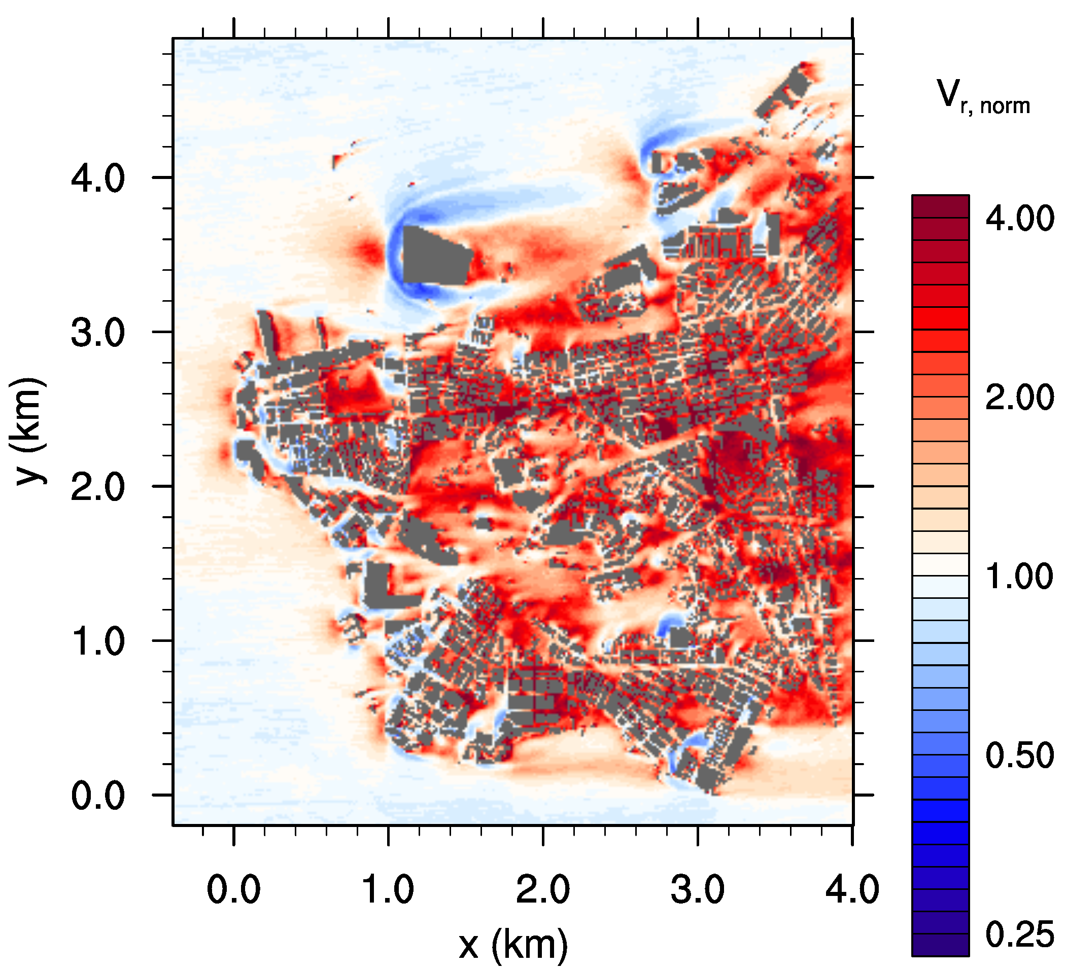
A better view of the differences in is shown in Figure 6, which shows the normalized velocity ratio
Within the city, was up to four times higher in the unstable case than in the neutral case. However, at the edges of the exposed buildings and at the windward edge of the city, was only about 0.6 times its value in the neutral case. In the neutral case, the buildings blocked the airflow and forced the air to circulate around them horizontally. For reasons of continuity, the air was accelerated at the edges and decelerated at the leeward side of the buildings. In the unstable case, however, stratification made it much easier for the blocked air to flow over the buildings. This significantly reduced the air volume that was forced around the buildings, thereby preventing a strong increase in around the exposed buildings. Furthermore, the enhanced vertical exchange in momentum due to convection led to higher at the leeward side of these buildings and was also responsible for the strong increase in within the city. The average was about twice as high in the unstable case than in the neutral case.
The increase in within the city area for the unstable case compared to the neutral case was also found by Yang and Li [13], who reported that flow rates through street canyons were higher in an unstable stratified atmosphere compared to those under conditions of neutral stratification. However, the reduction of in the vicinity of exposed buildings was not reported, which was because Yang and Li [13] only used a very simplified building setup that did not include exposed buildings.
Further effects of a change in stratification on the ventilation could be derived from correlations of with different building parameters. Figure 7a,b shows the scatter plot for and the average building height and for and the plan area index (building area divided by total area), respectively. For this, the city was divided into non-overlapping patches. The data points represent the average values within each of the patches. Data for the neutral and unstable cases are depicted by blue dots and red crosses, respectively.
Figure 7 shows that as most data points for the neutral case lay within and , while, for the unstable case, the majority of data points were within and . However, no significant correlation was found between and (Figure 7a). For both stratifications, the coefficient of determination is . This means that had almost no influence on in the neutral or unstable case. By contrast, Hang et al. [26] observed higher wind speed in a tall idealized building array compared to a shallower building array considering neutral stratification. The dependency found by Hang et al. [26] was related to perfectly aligned buildings channeling the flow within the idealized building arrays. In this case, higher buildings improved the channeling effect as a larger air volume was blocked at the front of the building array and forced into the streets. This effect was not observed in the simulations in this study, in which streets were randomly aligned to the wind direction.
Figure 7b shows the scatter plot for and . In the neutral and unstable cases, and show a negative correlation. This was also reported by Hang et al. [26] for the neutral case. An area with high described a dense built-up area with narrow streets where the wind velocity was significantly reduced resulting in a low . By contrast, a mostly open-space area, where was low, had less influence on the wind field and therefore was high in such areas.
However, determination of the correlation varied between the neutral case and the unstable case. In the neutral case, the correlation was weak as showed a high level of variation for a specific . This resulted in a low of . In the unstable case, the impact of on ventilation was significantly higher than in the neutral case as was , which resulted from less variation in for a given .
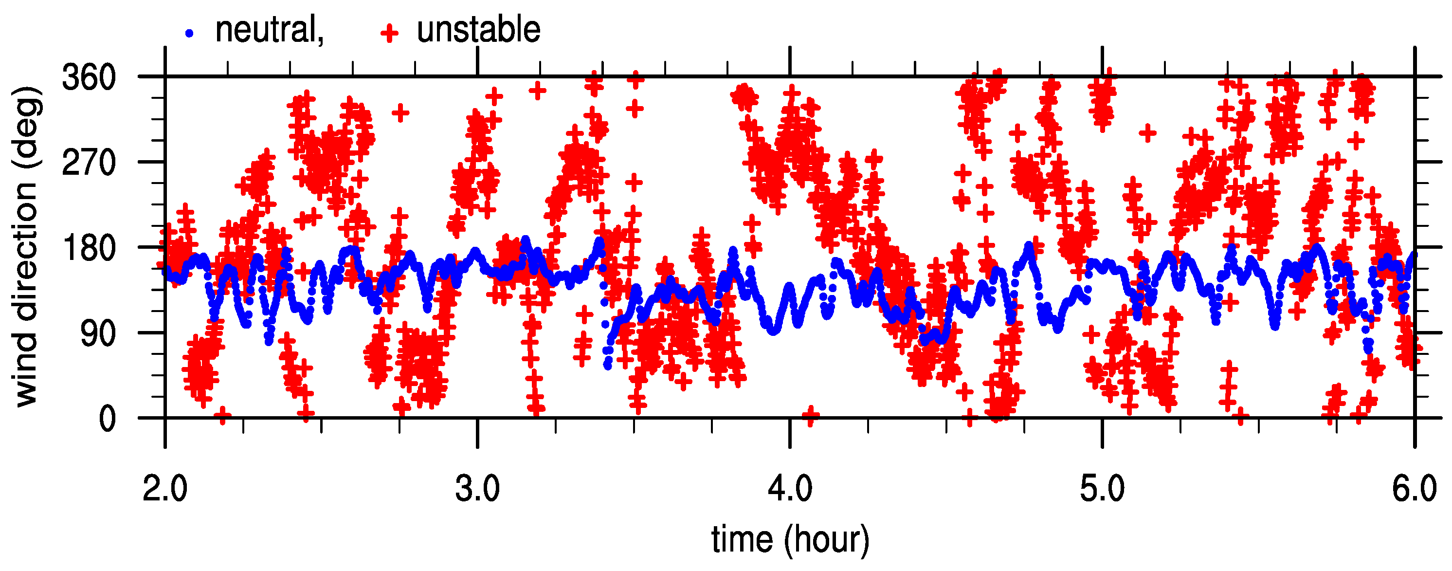
This difference in correlation between the two cases can be explained when considering the influence of the wind direction. In the neutral case, the ventilation was highly dependent on the orientation of the wind direction with regard to the orientation of the streets [27]. The wind direction changed only slightly at a given point in the neutral case. Figure 8 shows representative measurements of wind direction for both cases at position , which is the center of a street crossing within the city center. The wind direction varied between 54 and 188 for the neutral case, while the wind came from all directions in the unstable case. At the same time, the orientation of the streets within Kowloon was heterogeneous, with many patches existing with the same but different street orientations. Therefore, in the neutral case, some patches experienced good ventilation as their streets were oriented favorably for the given wind direction, while other patches constantly experienced unfavorable winds and therefore were poorly ventilated. Therefore, varied markedly in the neutral case for a given . As stated above, in the unstable case, ventilation was dominated by vertical mixing. Due to the strong convective motions and low background wind speed, the wind direction changed frequently (Figure 8). Therefore, the actual orientation of streets according to the wind direction was less important in the unstable case than in the neutral case. The main parameter determining the ventilation for the unstable case was therefore the amount of void space where convective motions could develop. This was related to , as it gave the ratio of occupied area to the total area. As , was the key parameter determining the ventilation for the unstable case.
4. Conclusions
This study compared ventilation in Kowloon City, Hong Kong, under conditions of neutral and unstable atmospheric stratification. For the comparison, a summer weak-wind situation with a geostrophic wind of 1.5 was chosen, as this condition was also the primary target of AVAs for Kowloon City.
An alternative definition of ventilation via the velocity ratio was presented. The standard definition considers the vertical distribution of wind velocity, and therefore depends on the stratification. The new definition neglected this vertical distribution and purely focused on the impact of obstacles under conditions of varying stratification, as it was directly calculated from the reduction of the wind velocity due to blockage of airflow by buildings. This enabled a better comparison of the influence of building on ventilation under different stratification conditions.
The averaged ventilation in the unstable case was about double that in the neutral case. This was due to the large convective eddies in the unstable case, which created a high degree of variation in wind direction and strong up- and downdrafts. The strong vertical motions reduced the decelerating impact of buildings on the flow field, as it was easier for the air to flow over them. However, this also reduced acceleration effects at the side edges of exposed buildings, which appeared in the neutral case. In these areas, was reduced to 0.6 times its value in the neutral case. Consequently, considering only neutral stratification when analyzing the ventilation of a city area was insufficient, as the ventilation appeared to be significantly changed, positively and negatively, under conditions of unstable stratification.
A linkage between the plan area index and was found similar to other studies for neutral stratification where low corresponds to high . However, the correlation between both variables was stronger in the unstable case than in the neutral case. In the neutral case, the correlation was reduced because, apart from , the orientation of the buildings in relation to the wind direction also influenced ventilation. In the unstable case, no distinct wind direction was present as it changed frequently due to the convective motions. This led to a smaller influence of the building orientation and a greater influence of on ventilation. Therefore, for cities where convective low-wind conditions are often present, such as Hong Kong, city planning should focus more on reducing to improve city ventilation than on the orientation of buildings and streets.
In contrast to other studies, no correlation was found between the average building height and . As these other studies only focused on idealized homogeneous block arrays, it is possible that the idealized cases overestimated the channeling induced by these idealized building arrays.
The results of this study indicated that AVAs should not focus purely on neutral stratification but should also consider unstable stratification, particularly when these conditions in combination with low wind speed are observed frequently, as in Hong Kong. When focusing on summer weak-wind conditions, a complete view on the ventilation of a city area can only be obtained if both neutral and unstable stratification are included in the analysis. For strong-wind conditions, the influence of mechanically induced turbulence may become stronger than that of thermally induced turbulence, which was already found by Yang and Li [13] for a very simplified city case.
The impact of stable stratification was not covered in this study but should be examined in future analyses. The first inspection of the impact of stable stratification on ventilation was made by Yang and Li [13] for a simplified city case. However, these results should be tested with a more realistic setup. The results of this study revealed differences between a simple building case and a more realistic setup for unstable stratification. Therefore, it is possible that results would also differ for a stable case with a more sophisticated building setup.
Surface elevation and land cover were neglected in this study to extract the pure influence of buildings on ventilation under different stratification conditions. Recent studies by Wolf-Grosse et al. [28] and Ronda et al. [18], however, showed the importance of topographic effects and consideration of water bodies at city scale. Therefore, these effects will be considered in a follow-up study, focusing on their combined influence on ventilation. In particular, the difference in land cover with resulting heterogeneous surface heat flux may have a large impact on ventilation as this leads to small-scale secondary circulations, such as sea breeze. A further step towards reality will also be to use an urban surface model available in PALM [29,30], which allows to accurately calculate surface temperatures based on a building-energy-balance model.
Supplementary Materials
The modified code parts used in addition to the standard code base of PALM are available online at www.mdpi.com/2073-4433/8/9/168/s1.
Acknowledgments
The authors thank Weiwen Wang, School of Architecture, Chinese University of Hong Kong, for providing the building data. The study was supported by a research grant (14408214) from General Research Fund of Hong Kong Research Grants Council (HK RGC-GRF). Tobias Gronemeier was supported by MOSAIK, which is funded by the German Federal Ministry of Education and Research (BMBF) under grant 01LP1601A within the framework of Research for Sustainable Development (FONA; http://www.fona.de). The simulations were performed with resources provided by the North-German Supercomputing Alliance (HLRN). NCL (The NCAR Command Language, Version 6.1.2, 2013 (Software), Boulder, Colorado: UCAR/NCAR/CISL/VETS, http://dx.doi.org/10.5065/D6WD3XH5) was used for data analysis and visualization. The PALM code can be accessed under https://palm.muk.uni-hannover.de. The publication of this article was funded by the Open Access fund of Leibniz Universität Hannover.
Author Contributions
T.G., S.R. and E.N. conceived and designed the simulations; T.G. performed the simulations; T.G. and S.R. analyzed the data; T.G. wrote the paper.
Conflicts of Interest
The authors declare no conflict of interest.
Appendix A
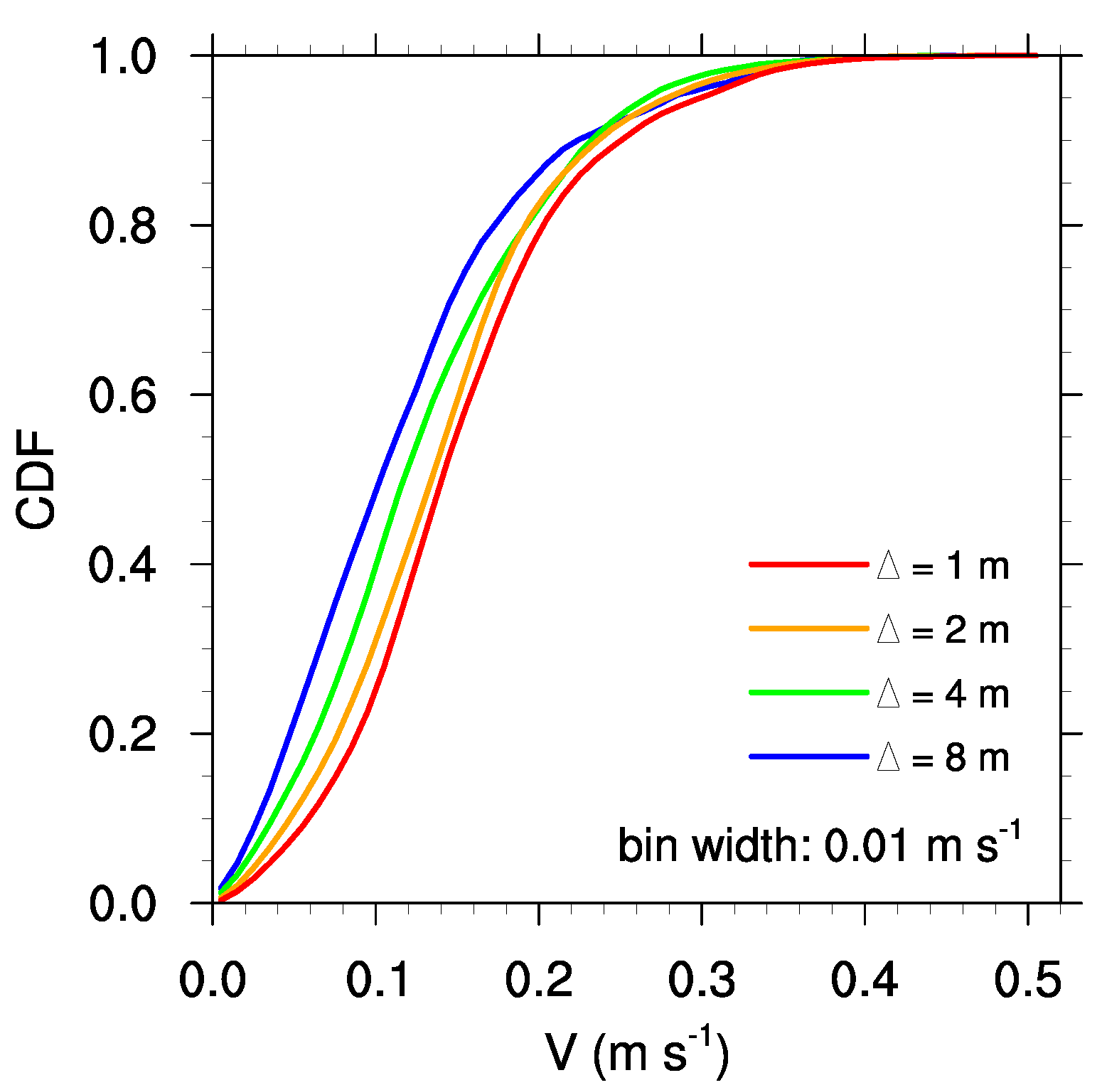
A grid sensitivity study was conducted to determine an appropriate grid width for the main simulations. Four simulations with grid sizes of 1 , 2 , 4 , and 8 were compared. The domain used in the sensitivity study included 1 km2 of Kowloon City. Cyclic boundary conditions and neutral stratification were used. As turbulent structures are generally larger in the unstable case than in the neutral case, the latter defined the minimum grid size to be used.
Figure A1 depicts the cumulative distribution function of the 1 averaged 3-dimensional wind velocity at a height of 4 for each simulation. Due to differences in grid level height between the simulations, data were linearly interpolated to . Significant differences in the distribution of V could be observed between 2 , 4 and 8 grid sizes. The distribution of low V decreased if a smaller grid size was used. The test statistic of Kuiper’s test [31], where compares the distribution function of case a to that of case b, yields , , and . Thus, the distribution of V changed significantly less if the grid size was reduced from 2 to 1 compared to a reduction from 8 to 4 or from 4 to 2 . Consequently, a reduction of grid size from 2 to 1 only slightly improved the quality of the representation of the wind field within the city. As a reduction of the grid size by a factor of 2 increased the computational load by a factor of 16 (double the grid points in each dimension multiplied by 2 for double the amount of time steps needed), a grid size of 2 was selected for the main simulations as a compromise between accuracy and computational cost.
Figure A1.
Cumulative distribution function of three-dimensional wind velocity V at 4 height. Data are averaged over 1 .
Figure A1.
Cumulative distribution function of three-dimensional wind velocity V at 4 height. Data are averaged over 1 .

References
- Xie, X.; Huang, Z.; Wang, J.S. Impact of building configuration on air quality in street canyon. Atmos. Environ. 2005, 39, 4519–4530. [Google Scholar] [CrossRef]
- Ng, E. Policies and technical guidelines for urban planning of high-density cities—Air ventilation assessment (AVA) of Hong Kong. Build. Environ. 2009, 44, 1478–1488. [Google Scholar] [CrossRef]
- Ng, E.; Yuan, C.; Chen, L.; Ren, C.; Fung, J.C.H. Improving the wind environment in high-density cities by understanding urban morphology and surface roughness: A study in Hong Kong. Landsc. Urban Plan. 2011, 101, 59–74. [Google Scholar] [CrossRef]
- Cheng, Y.; Lien, F.; Yee, E.; Sinclair, R. A comparison of large Eddy simulations with a standard k–ϵ Reynolds-averaged Navier–Stokes model for the prediction of a fully developed turbulent flow over a matrix of cubes. J. Wind Eng. Ind. Aerodyn. 2003, 91, 1301–1328. [Google Scholar] [CrossRef]
- Ashie, Y.; Kono, T. Urban-scale CFD analysis in support of a climate-sensitive design for the Tokyo Bay area. Int. J. Climatol. 2011, 31, 174–188. [Google Scholar] [CrossRef]
- Tominaga, Y. Visualization of city breathability based on CFD technique: Case study for urban blocks in Niigata City. J. Vis. 2012, 15, 269–276. [Google Scholar] [CrossRef]
- Yang, L.; Li, Y. City ventilation of Hong Kong at no-wind conditions. Atmos. Environ. 2009, 43, 3111–3121. [Google Scholar] [CrossRef] [Green Version]
- Yim, S.H.L.; Fung, J.C.H.; Lau, A.K.H.; Kot, S.C. Air ventilation impacts of the “wall effect” resulting from the alignment of high-rise buildings. Atmos. Environ. 2009, 43, 4982–4994. [Google Scholar] [CrossRef]
- Yuan, C.; Ng, E.; Norford, L.K. Improving air quality in high-density cities by understanding the relationship between air pollutant dispersion and urban morphologies. Build. Environ. 2014, 71, 245–258. [Google Scholar] [CrossRef]
- Letzel, M.O.; Helmke, C.; Ng, E.; An, X.; Lai, A.; Raasch, S. LES case study on pedestrian level ventilation in two neighbourhoods in Hong Kong. Meteorol. Z. 2012, 21, 575–589. [Google Scholar] [CrossRef]
- Park, S.B.; Baik, J.J.; Lee, S.H. Impacts of mesoscale wind on turbulent flow and ventilation in a densely built-up urban area. J. Appl. Meteorol. Climatol. 2015, 54, 811–824. [Google Scholar] [CrossRef]
- Park, S.B.; Baik, J.J. A Large-Eddy Simulation Study of Thermal Effects on Turbulence Coherent Structures in and above a Building Array. J. Appl. Meteorol. Climatol. 2013, 52, 1348–1365. [Google Scholar] [CrossRef]
- Yang, L.; Li, Y. Thermal conditions and ventilation in an ideal city model of Hong Kong. Energy Build. 2011, 43, 1139–1148. [Google Scholar] [CrossRef]
- Raasch, S.; Schröter, M. PALM-A large-eddy simulation model performing on massively parallel computers. Meteorol. Z. 2001, 10, 363–372. [Google Scholar] [CrossRef]
- Maronga, B.; Gryschka, M.; Heinze, R.; Hoffmann, F.; Kanani-Sühring, F.; Keck, M.; Ketelsen, K.; Letzel, M.O.; Sühring, M.; Raasch, S. The Parallelized Large-Eddy Simulation Model (PALM) version 4.0 for atmospheric and oceanic flows: Model formulation, recent developments, and future perspectives. Geosci. Model Dev. 2015, 8, 2515–2551. [Google Scholar] [CrossRef]
- Lo, K.W.; Ngan, K. Characterising the pollutant ventilation characteristics of street canyons using the tracer age and age spectrum. Atmos. Environ. 2015, 122, 611–621. [Google Scholar] [CrossRef]
- Park, S.B.; Baik, J.J.; Ryu, Y.H. A Large-Eddy Simulation Study of Bottom-Heating Effects on Scalar Dispersion in and above a Cubical Building Array. J. Appl. Meteorol. Climatol. 2013, 52, 1738–1752. [Google Scholar] [CrossRef]
- Ronda, R.; Steeneveld, G.; Heusinkveld, B.; Attema, J.; Holtslag, B. Urban fine-scale forecasting reveals weather conditions with unprecedented detail. Bull. Am. Meteorol. Soc. 2017. [Google Scholar] [CrossRef]
- Lund, T.S.; Wu, X.; Squires, K.D. Generation of Turbulent Inflow Data for Spatially-Developing Boundary Layer Simulations. J. Comput. Phys. 1998, 140, 233–258. [Google Scholar] [CrossRef]
- Kataoka, H.; Mizuno, M. Numerical flow computation around aeroelastic 3D square cylinder using inflow turbulence. Wind Struct. 2002, 5, 379–392. [Google Scholar] [CrossRef]
- Orlanski, I. A simple boundary condition for unbounded hyperbolic flows. J. Comput. Phys. 1976, 21, 251–269. [Google Scholar] [CrossRef]
- Miller, M.J.; Thorpe, A.J. Radiation conditions for the lateral boundaries of limited-area numerical models. Q. J. R. Meteorol. Soc. 1981, 107, 615–628. [Google Scholar] [CrossRef]
- Gryschka, M.; Fricke, J.; Raasch, S. On the impact of forced roll convection on vertical turbulent transport in cold air outbreaks. J. Geophys. Res. Atmos. 2014, 119, 12513–12532. [Google Scholar] [CrossRef]
- Atkinson, B.W.; Wu Zhang, J. Mesoscale shallow convection in the atmosphere. Rev. Geophys. 1996, 34, 403–431. [Google Scholar] [CrossRef]
- Larousse, A.; Martinuzzi, R.; Tropea, C. Flow Around Surface-Mounted, Three-Dimensional Obstacles. In Proceedings of the Turbulent Shear Flows 8: Selected Papers from the Eighth International Symposium on Turbulent Shear Flows, Munich, Germany, 9–11 September 1991; Durst, F., Friedrich, R., Launder, B.E., Schmidt, F.W., Schumann, U., Whitelaw, J.H., Eds.; Springer: Berlin/Heidelberg, Germany, 1993; pp. 127–139. [Google Scholar]
- Hang, J.; Li, Y.; Sandberg, M. Experimental and numerical studies of flows through and within high-rise building arrays and their link to ventilation strategy. J. Wind Eng. Ind. Aerodyn. 2011, 99, 1036–1055. [Google Scholar] [CrossRef]
- Kim, J.J.; Baik, J.J. A numerical study of the effects of ambient wind direction on flow and dispersion in urban street canyons using the RNG k-e turbulence model. Atmos. Environ. 2004, 38, 3039–3048. [Google Scholar] [CrossRef]
- Wolf-Grosse, T.; Esau, I.; Reuder, J. Sensitivity of local air quality to the interplay between small- and large-scale circulations: A large-eddy simulation study. Atmos. Chem. Phys. 2017, 17, 7261–7276. [Google Scholar] [CrossRef]
- Resler, J.; Krč, P.; Belda, M.; Juruš, P.; Benešová, N.; Lopata, J.; Vlček, O.; Damašková, D.; Eben, K.; Derbek, P.; et al. A new urban surface model integrated in the large-eddy simulation model PALM. Geosci. Model Dev. Discuss. 2017, 2017, 1–26. [Google Scholar] [CrossRef]
- Yaghoobian, N.; Kleissl, J.; Paw, U.K.T. An Improved Three-Dimensional Simulation of the Diurnally Varying Street-Canyon Flow. Bound.-Layer Meteorol. 2014, 153, 251–276. [Google Scholar] [CrossRef]
- Kuiper, N.H. Tests concerning random points on a circle. Indag. Math. 1960, 63, 38–47. [Google Scholar] [CrossRef]
Figure 1.
Domain setup for the (a) neutral case and (b) unstable case; building height information is depicted in (c). The dashed line marks the recycling area. The gray rectangle marks the city area shown in detail in (c).
Figure 1.
Domain setup for the (a) neutral case and (b) unstable case; building height information is depicted in (c). The dashed line marks the recycling area. The gray rectangle marks the city area shown in detail in (c).
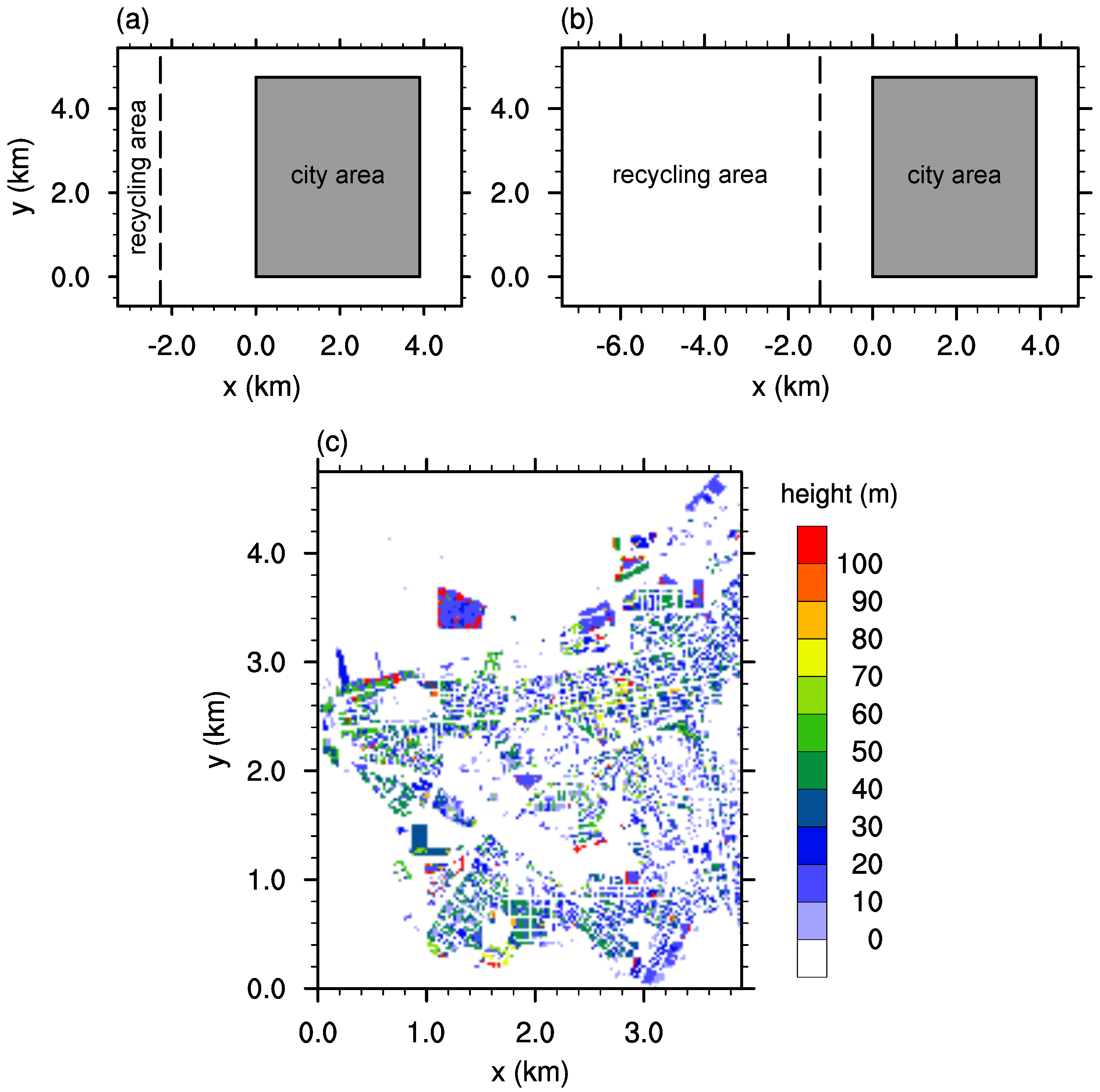
Figure 2.
Instantaneous vertical wind velocity (a) and potential temperature (b) for the unstable case after a simulation time of 6 at a height of 100 . The solid inner rectangle marks the city area.
Figure 2.
Instantaneous vertical wind velocity (a) and potential temperature (b) for the unstable case after a simulation time of 6 at a height of 100 . The solid inner rectangle marks the city area.
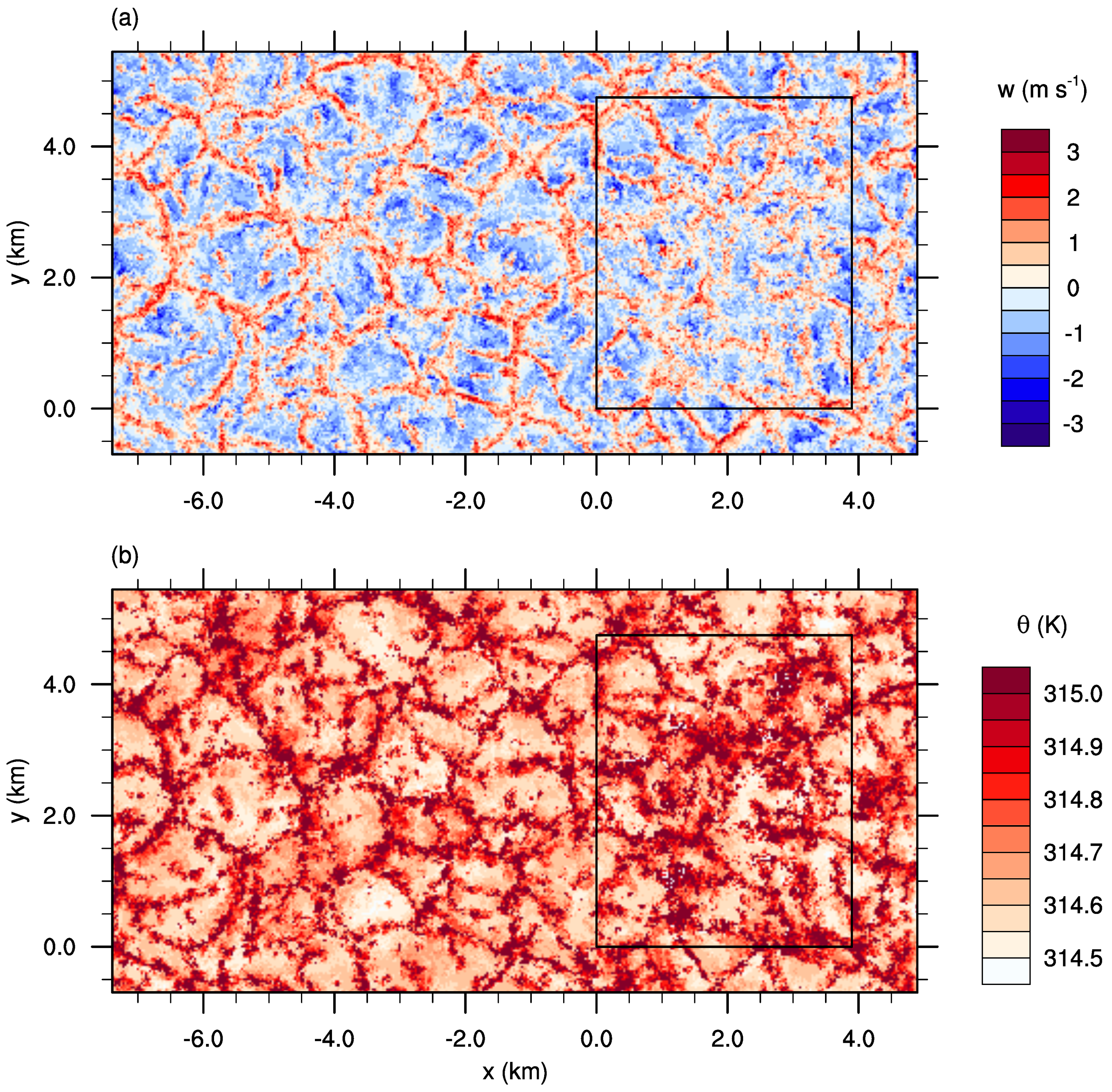
Figure 3.
Averaged three-dimensional wind velocity at 2 height for the (a) neutral case and (b) unstable case. Buildings are shown in gray.
Figure 3.
Averaged three-dimensional wind velocity at 2 height for the (a) neutral case and (b) unstable case. Buildings are shown in gray.
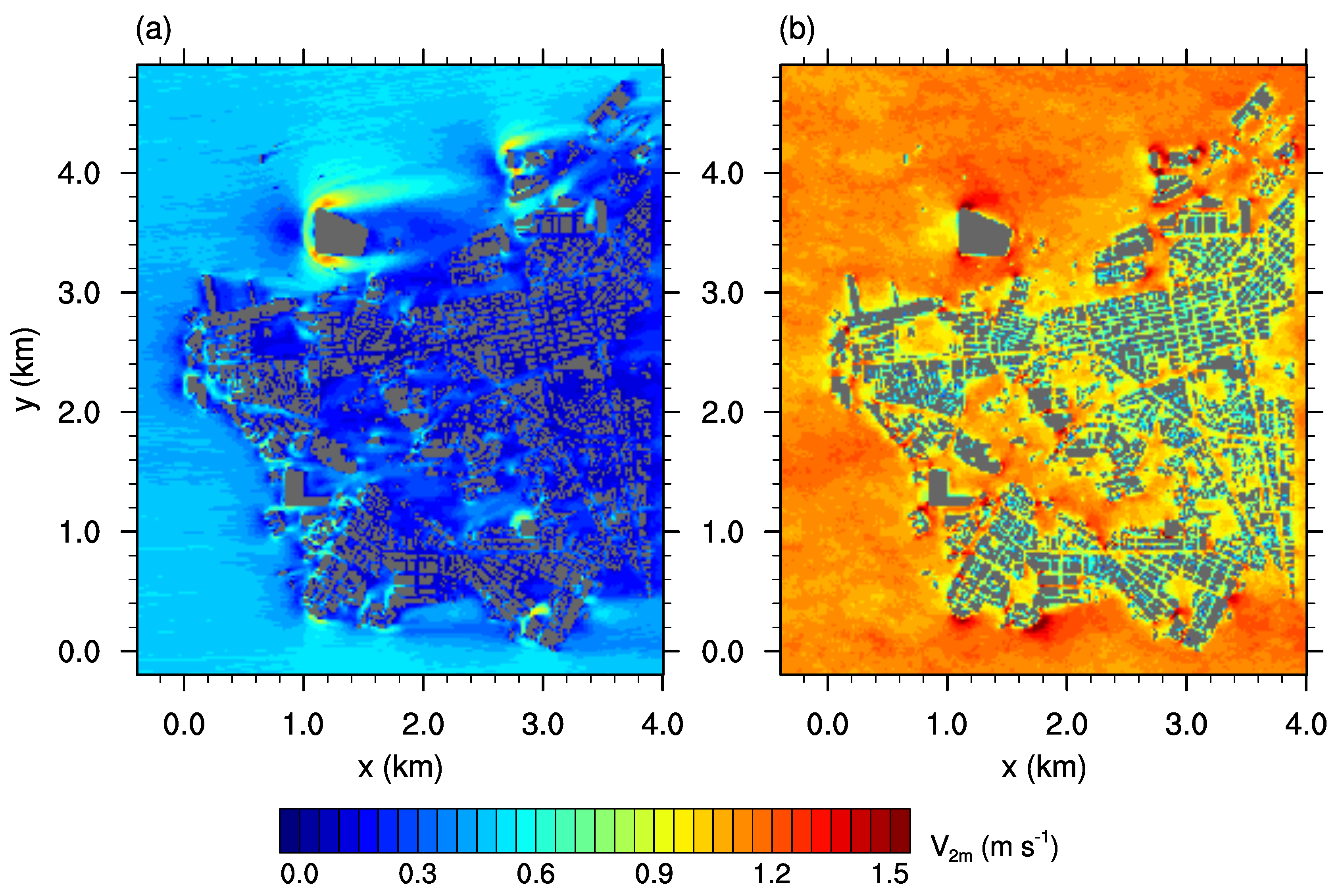
Figure 4.
Vertical profile of the wind speed of the mean horizontal wind vector within the recycling area.
Figure 4.
Vertical profile of the wind speed of the mean horizontal wind vector within the recycling area.
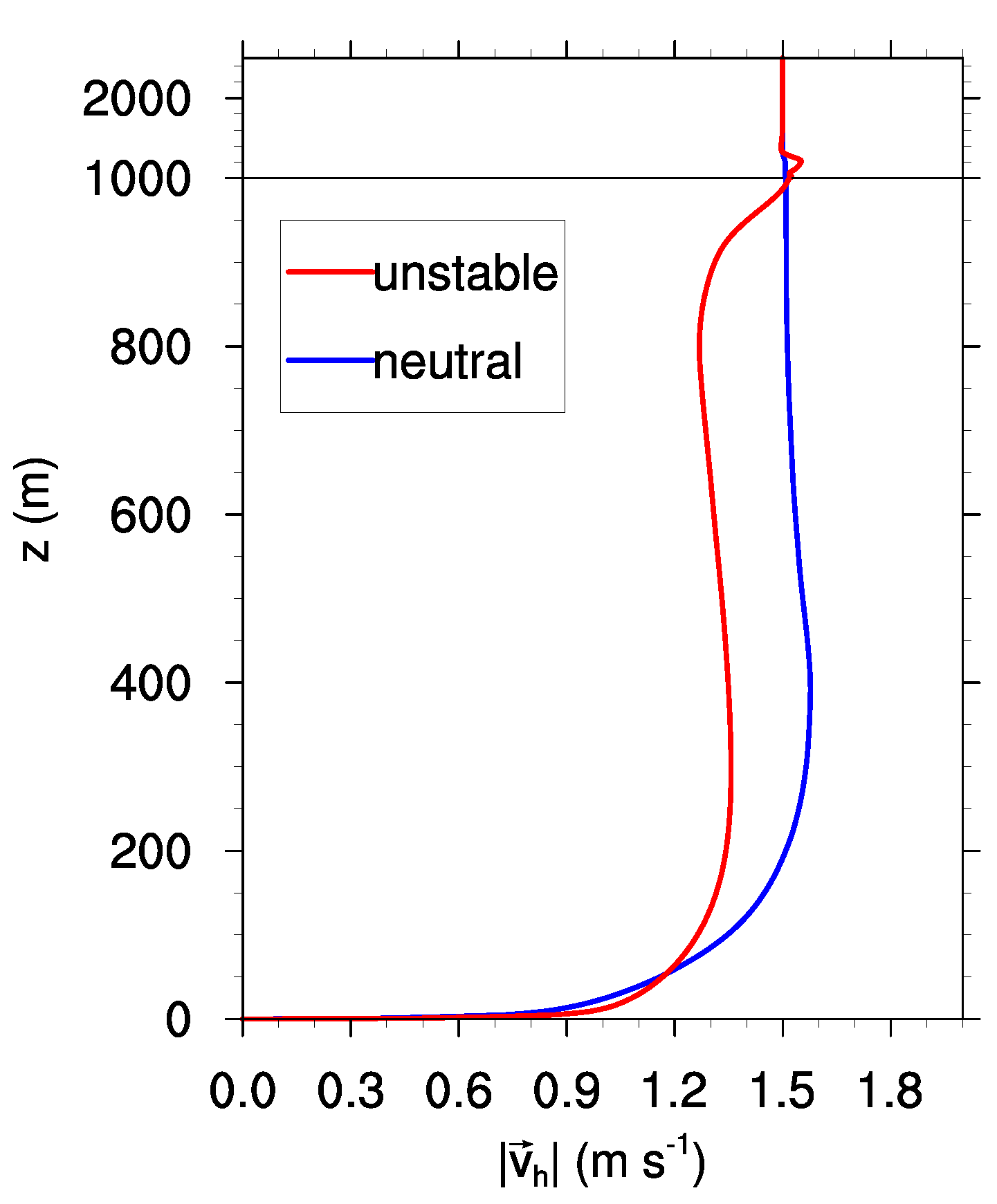
Figure 5.
Velocity ratio for the (a) neutral case and (b) unstable case.
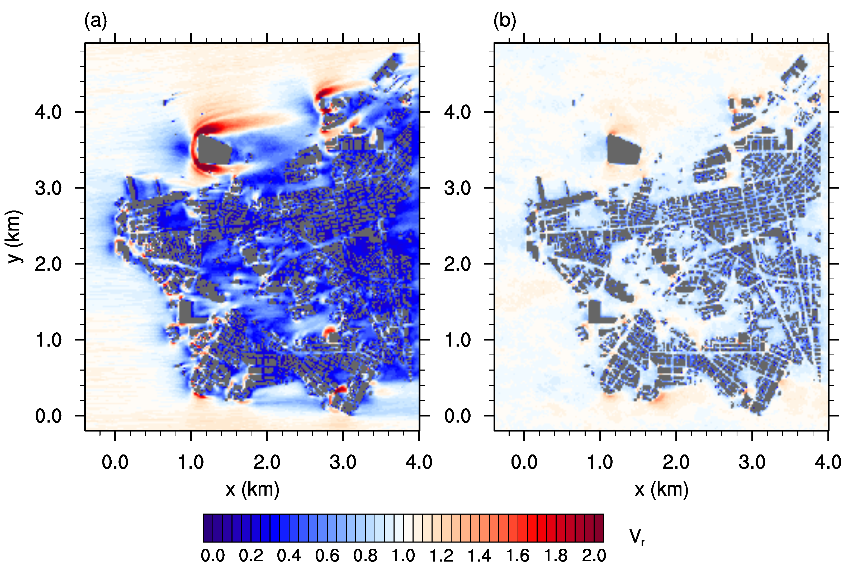
Figure 6.
Normalized velocity ratio . Values above 1 indicate higher in the unstable case, while values below 1 indicate higher in the neutral case.
Figure 6.
Normalized velocity ratio . Values above 1 indicate higher in the unstable case, while values below 1 indicate higher in the neutral case.

Figure 7.
Scatter plot for and (a) the average building height and (b) the plan area index . Each point represents an average value inside a area within the city. Blue dots represent the neutral case and red crosses represent the unstable case.
Figure 7.
Scatter plot for and (a) the average building height and (b) the plan area index . Each point represents an average value inside a area within the city. Blue dots represent the neutral case and red crosses represent the unstable case.
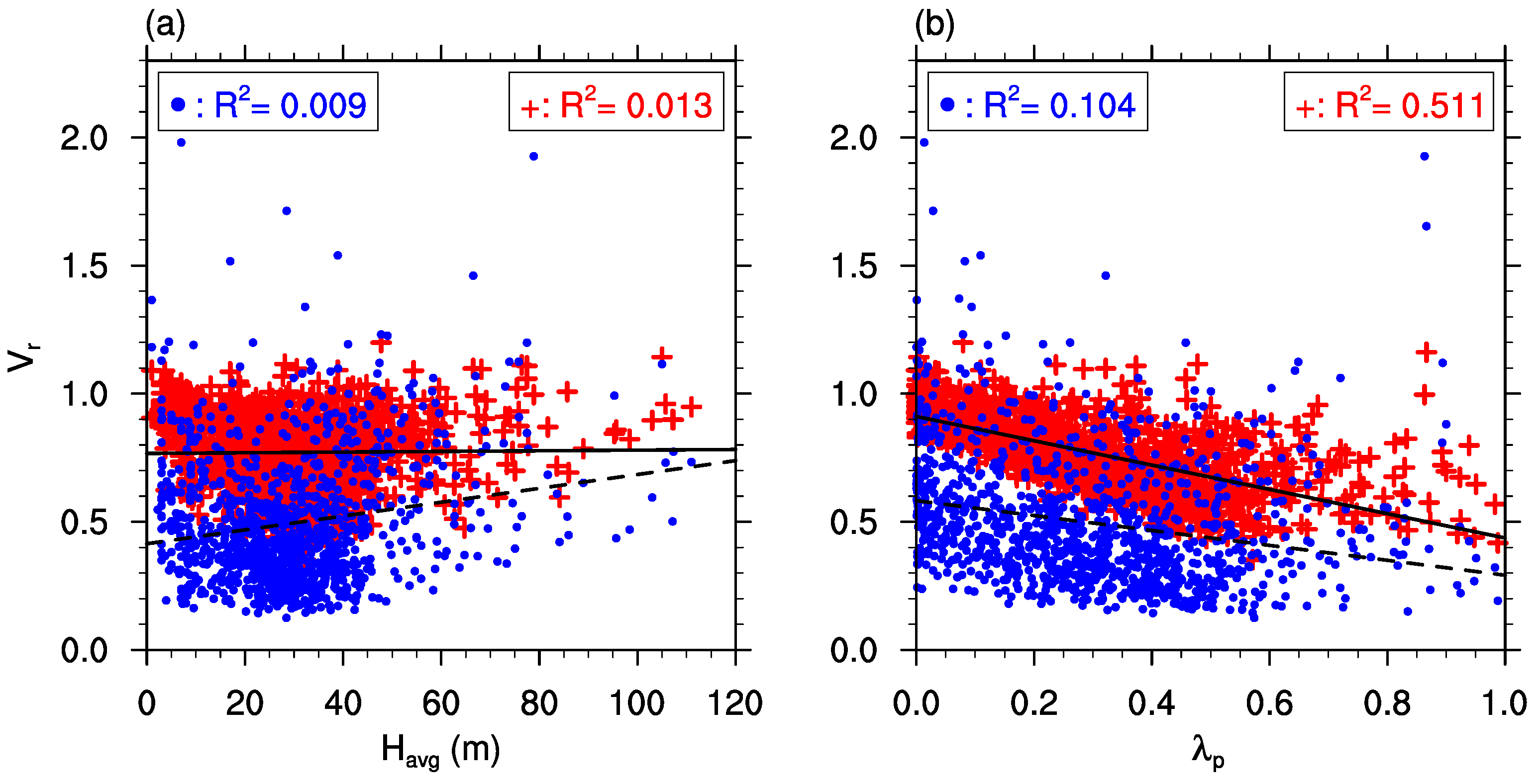
Figure 8.
Time series of wind direction at position in the city center. Blue dots represent the neutral case and red crosses represent the unstable case.
Figure 8.
Time series of wind direction at position in the city center. Blue dots represent the neutral case and red crosses represent the unstable case.

© 2017 by the authors. Licensee MDPI, Basel, Switzerland. This article is an open access article distributed under the terms and conditions of the Creative Commons Attribution (CC BY) license (http://creativecommons.org/licenses/by/4.0/).
Share and Cite
MDPI and ACS Style
Gronemeier, T.; Raasch, S.; Ng, E. Effects of Unstable Stratification on Ventilation in Hong Kong. Atmosphere 2017, 8, 168. https://doi.org/10.3390/atmos8090168
AMA Style
Gronemeier T, Raasch S, Ng E. Effects of Unstable Stratification on Ventilation in Hong Kong. Atmosphere. 2017; 8(9):168. https://doi.org/10.3390/atmos8090168
Chicago/Turabian StyleGronemeier, Tobias, Siegfried Raasch, and Edward Ng. 2017. "Effects of Unstable Stratification on Ventilation in Hong Kong" Atmosphere 8, no. 9: 168. https://doi.org/10.3390/atmos8090168
Note that from the first issue of 2016, this journal uses article numbers instead of page numbers. See further details here.