The Impact of Planting Trees on NO_x Concentrations: The Case of the Plaza de la Cruz Neighborhood in Pamplona (Spain)

Abstract

In this paper, the role of trees on airborne pollutant dispersion in a real neighborhood in Pamplona (Spain) is discussed. A Computational Fluid Dynamics (CFD) model is employed and evaluated against concentrations measured during the last part of winter season at a monitoring station located in the study area. Aerodynamic and deposition effects of trees are jointly considered, which has only been done in few recent studies. Specifically, the impact on NO_x concentration of: (a) tree-foliage; and (b) introducing new vegetation in a tree-free street is analyzed considering several deposition velocities and Leaf Area Densities (LAD) to model deciduous and evergreen vegetation. Results show that the higher the LAD, the higher the deposition (concentration reduction) and the blocking aerodynamic effect (concentration increase). Regardless of foliage or deposition rates, results suggest the predominance of aerodynamic effects which induce concentration increases up to a maximum of 7.2%, while deposition induces concentration decreases up to a maximum of 6.9%. The inclusion of new trees in one street modifies the distribution of pollutant, not only in that street, but also in nearby locations with concentration increase or decrease. This finding suggests that planting trees in street with traffic as an air pollution reduction strategy seems to be not appropriate in general, highlighting the necessity of ad hoc studies for each particular case to select the suitable location of new vegetation.

1. Introduction

In urban areas, air quality problems usually occur due to reduced ventilation and high pollutant concentrations. Traffic emissions generally constitute the major source of air pollution and roadside barriers can be employed to influence flow patterns and, thus, the resulting levels of concentrations. Advantages and disadvantages of using several barriers, such as trees and vegetation, noise barriers, low boundary walls, and parked cars, have been recently reviewed by Gallagher et al. [1].

In urban areas, vegetation has been shown to exert several ecosystem services, such as carbon sequestration, micro-climate regulation, noise reduction, rainwater drainage, improvement of mental health, and recreational values, as well as changes in air pollution. A recent research overview on the impacts of urban trees on water, heat, and pollution cycles has been given by Livesley et al. [2]. They summarized 14 studies attempting to provide a global perspective on the ecological services of trees in towns and cities from five continents. The complexity of the ecosystem service valuation has still prevented comprehensive investigations for specific areas and thus, further studies in urban areas are still needed [3].

Among the ecosystem services, the impact on urban air pollution, which is the focus of the present paper, has been documented in several studies, but not yet completely established. Flow and pollutant dispersion in the presence of vegetation (mainly trees) is an up-to-date research using field (e.g., [4,5,6,7,8,9,10,11,12,13]) and wind tunnel (e.g., [14,15,16,17]) investigations. Several studies, recently reviewed by Janhäll [18], Salmond et al. [19], Grote et al. [3], and Abhijith et al. [20], have shown the potential of vegetation in mitigating air pollution, but also has left open questions on the the impact that street trees have on air quality in urban areas and street canyons, since they may lead to increased or decreased concentrations.

Specifically, as summarized by Grote et al. [3], positive impacts of trees on air quality occur due to the deposition of pollutants on plant surfaces and stomatal uptake. If the stomata are closed, gaseous, and particle deposition mostly occurs at leaf surfaces. Together with pollutants that are bind to or destroyed at the outer surface, uptake into leaves occurs through the stomata and such a mechanism is enhanced if compounds are removed from intercellular spaces. In general, deposition rates depend on pollutant concentrations, meteorological conditions, air movement through the crown, transfer through the boundary layer adjacent to surfaces, and absorption capacity of surfaces, which also depend on stomatal conductance. In turn, these depend on species, arrangement, crown, and foliage characteristics. Pollutant removal from the atmosphere also occurs through the influence on microclimates as temperature reductions by shade and evapotranspiration may change the rate of chemical reactions, leading to reduced concentrations of ozone.

On the other hand, the negative impacts of trees on air quality are due to the release of allergenic particulates and harmful volatile organic compounds that can act as a precursor to smog or ozone formation, particularly when NO_x is present and climatic conditions are favorable. Further, vegetation, and in particular trees, may obstruct the air exchange and dispersion of traffic-related pollutants, and increase concentrations in the lower region below the crowns of trees, especially when they are characterized by high leaf area density (LAD). One of the pioneering experiments was that performed in the wind tunnel of the University of Karlsruhe. Aerodynamic effects of trees were found to increase wall-averaged concentrations of isolated symmetric street canyons up to about 100%. Results also showed that street-level concentrations depend on wind direction and aspect ratio [14]. On the other hand, Gromke et al. [17] showed a reduction up to 60% at pedestrian level in the presence of continuous hedgerows using the same wind tunnel set-up.

Based on field and wind tunnel investigations, which were also used for validation purposes, several modelling techniques, especially Computational Fluid Dynamics (CFD), were also applied. Both aerodynamic [21,22,23,24,25] and deposition effects of trees [26,27,28,29,30] were considered within idealized and real scenarios. Modelling such effects of trees in microscale models is always a challenge since several mechanisms have to be taken into account simultaneously—for particles, emitted gases, and ozone, the challenges are different. As for aerodynamic effects, trees are usually considered as porous media and additional terms are added to the momentum and turbulence equations, while the deposition is modelled as a volumetric sink term in the transport equation of pollutants. This term is proportional to LAD, deposition velocity, and air pollutant concentration. As mentioned above, the values of deposition velocity depend on the type of vegetation and pollutant. Many discrepancies between published values are found [18]. Deposition velocities for vegetated surfaces are usually less than 1 cm s⁻¹ for some gases to several cm s⁻¹ for particles.

Many modelling studies found that aerodynamic effects of trees are more significant than deposition [26,27,31], even though Santiago et al. [28] reported decreased concentrations close to the ground up to 60% in several idealized arrays of different packing density depending on tree location, LAD, and deposition velocity. They showed that the deposition effects are also crucial in determining the final concentration levels. Positive effects were also reported by Jeanjean et al. [26,27], who found that trees are beneficial from a purely dynamic point of view, with a concentration decrease of 7% on average at pedestrian height in the neighbourhoods of Leicester and London (UK).

Even though challenges and strategies for urban green-space planning in compact cities have also been proposed [32], it can be argued that the effects of urban vegetation strictly depend on their interaction with the city morphology and meteorological conditions. Currently, studies which account for the main effects of trees (aerodynamic, deposition and thermal) are still poor in the literature and thus, comprehensive strategies on the use of urban vegetation for air quality purposes are still missing [1].

It is worth noting that in the modelling studies aerodynamic and deposition effects of trees have been separately investigated using simple geometries, and only few recent studies bring them together. However, these studies have not quantified the relative influences of both effects on pollutant concentration in real scenarios. In this perspective, the purpose of this work is: (a) to determine the influence of aerodynamic and deposition effects on NO_x concentrations in a real neighborhood; and (b) to evaluate the impact of introducing new trees as mitigation strategy of air pollution. A CFD model with a Reynolds-Averaged Navier-Stokes (RANS) closure evaluated against data monitored from an air quality station of the Regional Government of Navarra (Spain) network is used to achieve this purpose. The focus is on rush hour conditions in winter, because higher levels of NO_x are usually found for these cases. Specifically, starting from the real scenario of deciduous trees (low LAD), the impact on NO_x concentration of: (a) tree-foliage of different LAD; and (b) new trees planted in the neighborhood, as well as the importance of deposition and aerodynamic effects in each case, is analyzed.

2. Description of Study Area, Modelling Set-Up and Investigated Scenarios

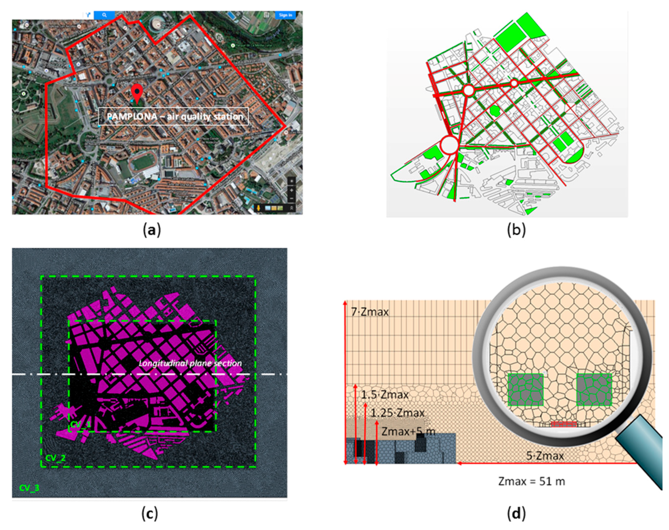
2.1. The Study Area and Modeling Set-Up

The study area is located at the II Ensanche neighbourhood of Pamplona (Spain), whose diameter is about 1.3 km (Figure 1a). The height of buildings ranges from 11 m to 51 m, with a mean height of 20 m. An air quality (AQ) monitoring station is located in a square in the centre of the neighbourhood. The extent of vegetation in the zone, in terms of plan area (i.e., the extent of vegetation projected in a horizontal plane respect to the total plan area of the streets and squares), is 13.8%. There are trees in most of the streets and small parks (Figure 1a). Due to the lack of specific tree data, the mean height of trees was estimated through satellite images from Google Earth^® and ranges from 5 m to 12 m.

The CFD model used was the code Star-CCM+ from CD-Adapco (London, UK) [24,28,34] solves Reynolds-averaged Navier-Stokes (RANS) equations with the Realizable k-ε turbulence model, where k is the turbulent kinetic energy and ε is the dissipation of turbulent kinetic energy. A transport equation is used to simulate the dispersion of nitrogen oxides (NO_x), where diffusivity is related to turbulent viscosity divided by Schmidt number (Sc). Dispersion of NO_x (regarded as NO + NO₂) is modelled in order to avoid the inclusion of chemical reactions in the CFD simulations since NO_x can be considered as a non-reactive gas [24,35,36]. The aerodynamic effects of vegetation are modelled by means of a sink in the momentum equation ($S{u}_i$, Equation (1)) and sinks/sources in turbulence equations ($S_k$ and $S_{\epsilon }$, Equations (2) and (3)). In addition, the fraction of pollutant removed from air by means of the deposition to the leaves is represented as a mass sink in the transport equation ($S_d$, Equation 4). This approach to model vegetation has been evaluated by Santiago et al. [24], Krayenhoff et al. [37], and Santiago et al. [28], and it is also similar to those employed in other CFD studies [23,25,31]. The mathematical expressions are the following,

$$S{u}_i=-\rho LAD{c}_{d}U{u}_i$$

(1)

$$S_k=-\rho LAD{c}_d\left({\beta }_p{U}^3-{\beta }_{d}Uk\right)$$

(2)

$$S_{\epsilon }=-\rho LAD{c}_d(C_{\epsilon 4}{\beta }_p\frac{ϵ}{k}{U}^3-C_{\epsilon 5}{\beta }_{d}U\epsilon )$$

(3)

$$\mathrm{m}{S}_d=-LAD v_{dep}C\left(x,y,z\right)$$

(4)

where $\rho$ is the air density, $c_d$ is the sectional drag coefficient for vegetation (=0.2), $U$ is the wind speed, $u_i$ is the velocity component in direction i, ${\beta }_p$ is the fraction of mean kinetic energy converted into turbulent kinetic energy, ${\beta }_d$ is the dimensionless coefficient for the short-circuiting of turbulent cascade, $C_{\epsilon 4}$ and $C_{\epsilon 5}$ are model constant, $v_{dep}$ is deposition velocity and $C\left(x,y,z\right)$ is the concentration at position (x, y, z). Values of ${\beta }_d$, $C_{\epsilon 4}$ and $C_{\epsilon 5}$ are based on analytical expressions [38] with ${\beta }_p=1$ as in Santiago et al. [28].

$${\beta }_d=C_{\mu }^{0.5}{\left(\frac{2}{\alpha }\right)}^{\frac{2}{3}}{\beta }_p+\frac{3}{{\sigma }_k}$$

(5)

$$C_{\epsilon 4}\left(=C_{\epsilon 5}\right)={\sigma }_k\left(\frac{2}{{\sigma }_{\epsilon }}-\frac{C_{\mu }^{0.5}}{6}{\left(\frac{2}{\mathsf{\alpha }}\right)}^{\frac{2}{3}}\left(C_{\epsilon 2}-C_{\epsilon 1}\right)\right)$$

(6)

We assume $C_{\epsilon 4}=C_{\epsilon 5}$ and use α = 0.05 and $(C_{\mu },{\sigma }_k,{\sigma }_{\epsilon },C_{\epsilon 1},C_{\epsilon 2}=\left(0.09,1,1.3,1.44,1.92\right)$.

The geometry of each building has been obtained from a 2D map of the city in CAD format where each building is extruded considering its height. This real neighbourhood configuration has been imported to the CFD model. Specifically, geometry models for trees and traffic sources have been set up from satellite images from Google Earth^® [39]. For simplicity, only rows of trees have been considered instead of individual trees. Trees are placed through the streets, and the base and the top of the crown are located depending on the type of tree within each street by using Google Earth^® information. The bases and the tops of tree crowns range from 2 m to 4 m, and 5 m to 12 m, respectively. In the virtual case (i.e., where new vegetation is introduced in one tree-free street), the base and the top of the crown are located at 4 m and 10 m, respectively, which are consistent with those of trees located within the parallel street. Traffic emissions are distributed along the streets and the width is determined by the number of lanes (e.g., 3.5 m wide for one-way street, 7 m wide for two-way street and so on). Also, it is assumed that traffic emissions height is 1 m above the ground (Figure 1b) in order to take the initial dispersion into account.

The domain size has been built according to the best practice guidelines [40]. The height of the domain is 7 Zmax, where Zmax is the height of the tallest building (50 m). The distance between buildings and inlet and outlet boundaries are larger than 8 times the building heights. Note that, except the tallest building, the average height of most of the buildings is around 20 m.

The choice of the mesh has been made based on grid sensitivity tests. The domain has been discretized using polyhedral cells. It is made up of 3 control volumes (CV_1, CV_2, and CV_3) of characteristic sizes: 2.7 m, 6.7 m, and 10 m, respectively (Figure 1c). Further, a prism layer of hexahedral cells around buildings (of about 1 m) and ad hoc refinements in the narrowest streets have been added. Polyhedral and structure grids are combined in order to optimize the number of grid cells and save computational cost. Figure 1d shows the gradual shifting between control volumes at a longitudinal plane. The total number of cells is 7.4 × 10⁶ cells. In order to check the independence of numerical results on the grid size, two finer meshes have been evaluated: mesh 2 with control volumes characteristic sizes of 2 m, 5 m, and 10 m, respectively. Mesh 3 which characteristic sizes are 1.5 m, 3.8 m, and 10 m, respectively. Vertical profiles of wind speed and turbulent kinetic energy in three different locations have been analysed in this test. The differences found against the results from the three grid resolutions are insignificant, and the first mesh is considered appropriate.

Concerning boundary conditions, building, and ground are modelled as walls. At the top of domain symmetry, boundary conditions are considered to establish zero normal velocity and zero normal gradients of all variables at this plane. Neutral inlet profiles of velocity, turbulent kinetic energy (k), and dissipation of turbulent kinetic energy (ε) are computed by the following equations [21,24,41,42]:

$$u\left(z\right)=\frac{u_{*}}{\kappa }\ln \left(\frac{z+z_0}{z_0}\right)$$

(7)

$$k=\frac{u_{*}^2}{\sqrt{C_{\mu }}}$$

(8)

$$\epsilon =\frac{u_{*}^3}{\kappa \left(z+z_0\right)}$$

(9)

where u_* is the friction velocity, z₀ is the roughness length, C_µ is a model constant (=0.09) and κ is von Karman’s constant (κ = 0.4). This approach is acceptable for winter season [24,42].

2.2. Description of Investigated Scenarios

Several scenarios, both real and virtual, have been investigated. First, the real scenario is evaluated against data monitored during two weeks from the AQ monitoring station (located at 3 m a.g.l.). For this, time average NO_x concentrations are computed.

Winter has been selected because levels of NO_x measured at the AQ station in the study area are usually higher than in other seasons. As for LAD, over the year, LAD of deciduous vegetation changes, and for instance in winter, is almost 0. With this in mind, the month of March 2015 has been chosen, when LAD (=0.1 m²m⁻³) is low, but not 0, and NO_x levels are still high. This LAD has been selected according to a preliminary study performed by Rivas et al. [43] in the same area. They evaluated NO_x concentration during different time periods considering LAD = 0 (no trees), 0.1 and, 0.5 m²m⁻³, concluding that the fit with experimental values was better for cases with LAD = 0.1 m²m⁻³ in winter and with LAD = 0.5 m²m⁻³ in summer. Note that the values of LAD used in the study are slightly low in comparison with the literature [44]. This is because trees have been modelled by means of rows of trees and not as individual trees. Therefore, this value includes LAD for trees and the gap between them, which is different to the real LAD of an individual tree.

Second, the study focuses on the worst case in terms of air quality. The maximum values of NO_x concentrations have been found at 8 a.m., which correspond to the maximum of traffic emissions in these streets during the day. Taking this into account, the focus is on NO_x dispersion under these adverse conditions. Meteorological data obtained from a station located close to the neighborhood have been used to simulate the typical meteorological conditions at this hour. Under these adverse conditions, the impact of deposition and aerodynamic effects of trees on pollutant concentrations has been analyzed, as well as the effect of increasing LAD or planting new trees. To analyze a wide range of deposition velocities, four deposition values were considered: 0, 0.005, 0.01, and 0.03 m s⁻¹. The objective is not to employ a specific and accurate value of deposition velocity, but to analyze the impact of vegetation on pollutant concentration for several scenarios with different realistic deposition velocities. This allows us to generalize the results for different deposition conditions as performed in Santiago et al. [25] for idealized scenarios. Specifically, the analysis focuses on:

a)

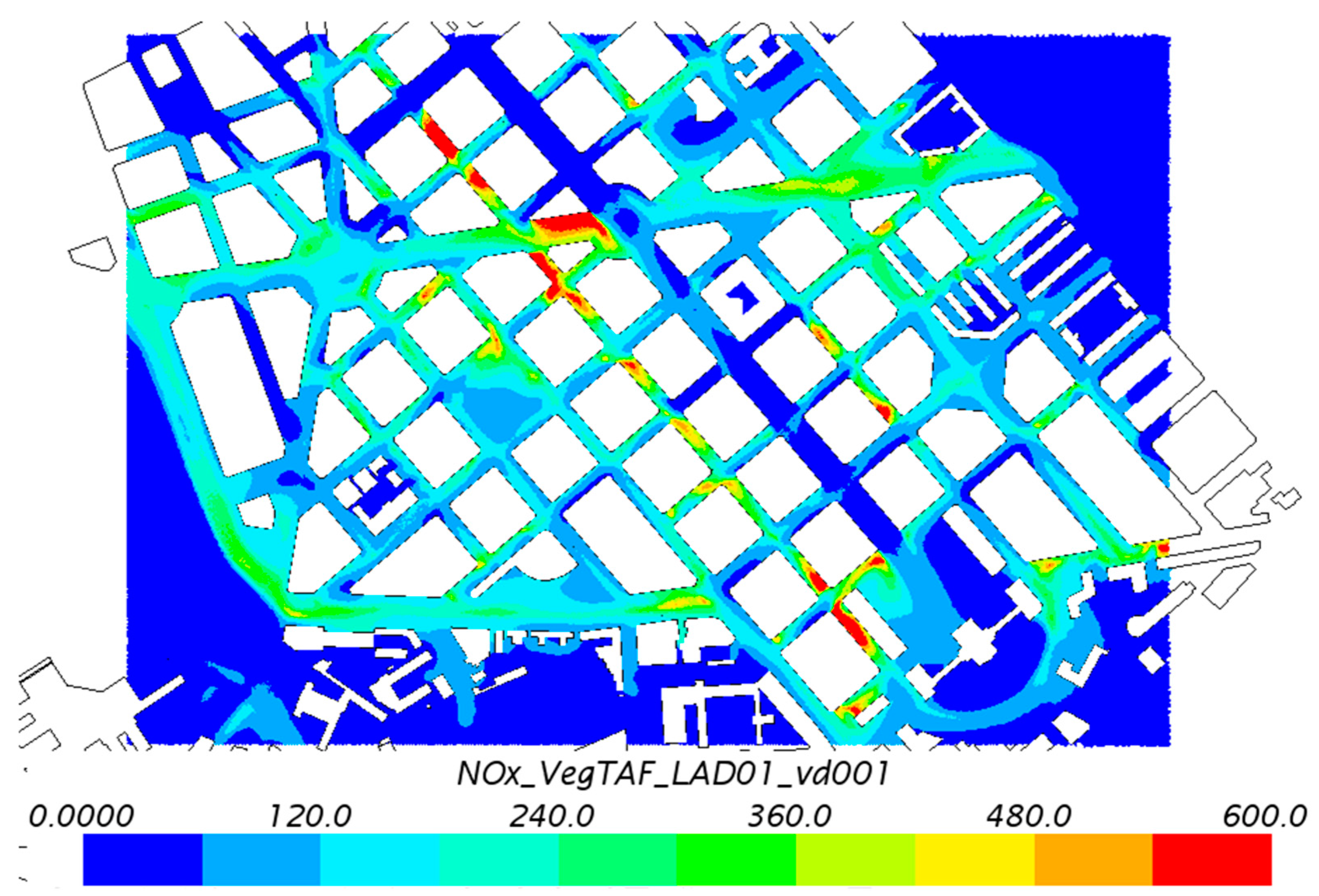
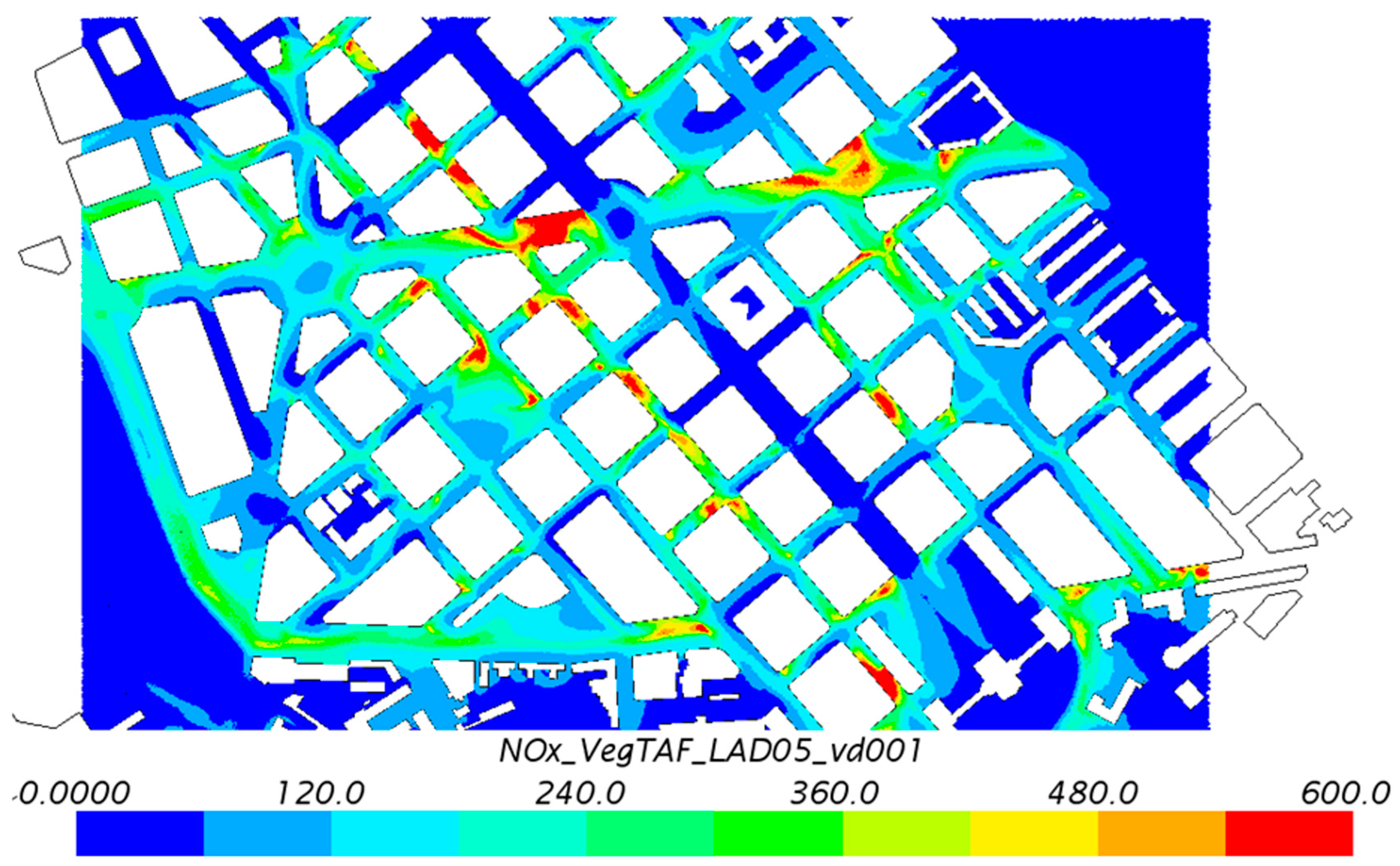
The effects of tree-foliage on concentration. LAD = 0.1 and 0.5 m²m⁻³ have been used to model deciduous vegetation in real cases and evergreen vegetation in virtual cases, respectively;

b)

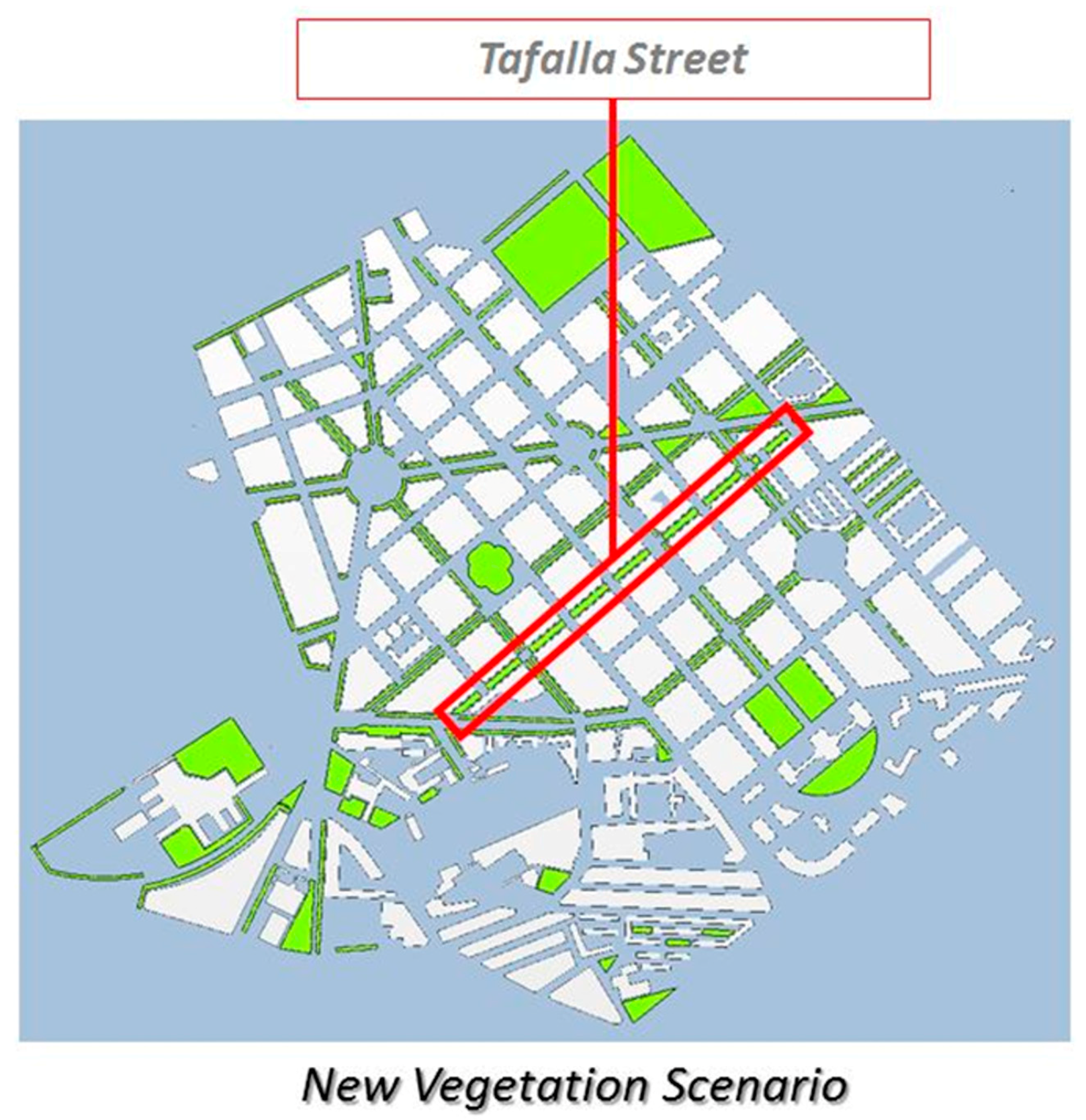
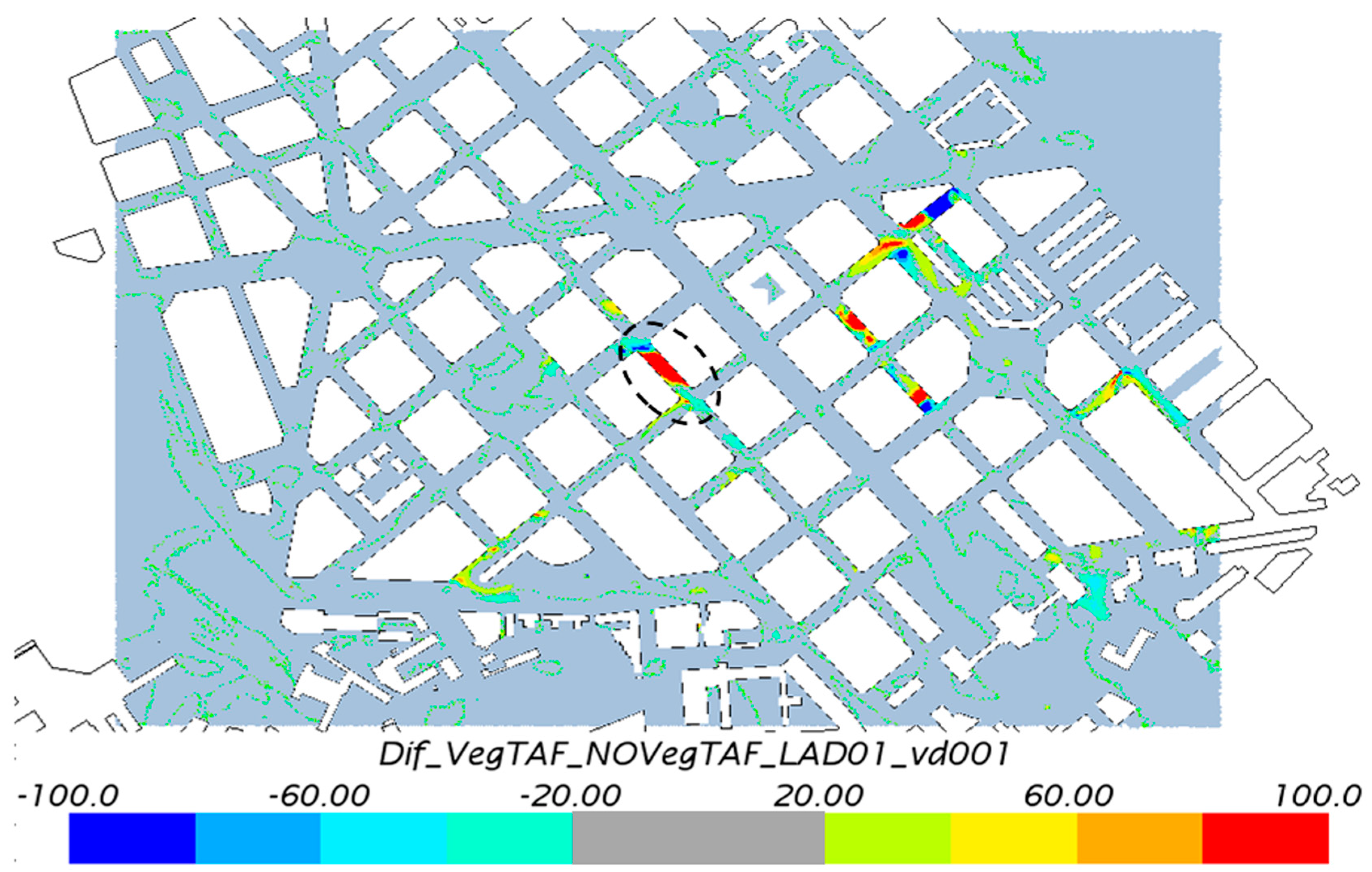
The effects on concentration of introducing new vegetation in a tree-free street.

Table 1. Description of investigated scenarios.

Scenario	Location of Vegetation	Type of Vegetation	Deposition Velocity (m s−1)
Current-1.a	Current location	Deciduous (LAD = 0.1 m2m−3)	0
Current-1.b			0.005
Current-1.c			0.01
Current-1.d			0.03
Current-2.a	Current location	Evergreen (LAD = 0.5 m2m−3)	0
Current-2.b			0.005
Current-2.c			0.01
Current-2.d			0.03
New-1.a	New trees in one tree-free street	Deciduous (LAD = 0.1 m2m−3)	0
New-1.b			0.005
New-1.c			0.01
New-1.d			0.03
New-2.a	New trees in one tree-free street	Evergreen (LAD = 0.5 m2m−3)	0
New-2.b			0.005
New-2.c			0.01
New-2.d			0.03

summarizes the studied scenarios which we expect to provide a decision support to urban planners for the selection of appropriate tree species and planting new trees.

3. CFD Modelling Evaluation

3.1. Previous Validation Studies

A detailed validation of the CFD-RANS simulations using real local data has not been possible, since only one AQ monitoring station from Regional Government of Navarra is located in the study area, specifically in a square in the centre of the neighbourhood. Therefore, the modelling approach employed here has been evaluated with data available from wind tunnel experiments by Brunet et al. [45] and Raupach et al. [46] for a “continuous” forest and a “forest” edge. These experiments have been extensively used to validate simulations with RANS by Foudhil et al. [47] and with Large Eddy Simulations by Dupont and Brunet [48]. Our validation results have been presented in Krayenhoff et al. [37] and Santiago et al. [28]. In addition, the current modelling of urban vegetation was evaluated by using CODASC wind-tunnel dataset (COncentration DAta of Street Canyons - www.windforschung.de/CODASC.htm) [49,50] by simulating a street canyon with and without vegetation. Two different tree porosities were used with a pressure loss coefficient (λ) of 80 and 200 m⁻¹ (0.53 and 1.33 m⁻¹ at full scale). Considering a drag coefficient of 0.2, these values correspond to LAD = 2.6 and 6.6 m²m⁻³, respectively. Overall, a slight overestimation of concentration was obtained [28]. Similar behavior was found by other studies using RANS [51,52,53] and LES [54]. Better results were obtained for a small Schmidt number (Sc = 0.3).

Based on the validation studies mentioned above, we are confident that the CFD model employed is able to reproduce the NO_x dispersion in the real scenario with vegetation and thus, the impact of several tree foliage densities or planting new trees has been quantified.

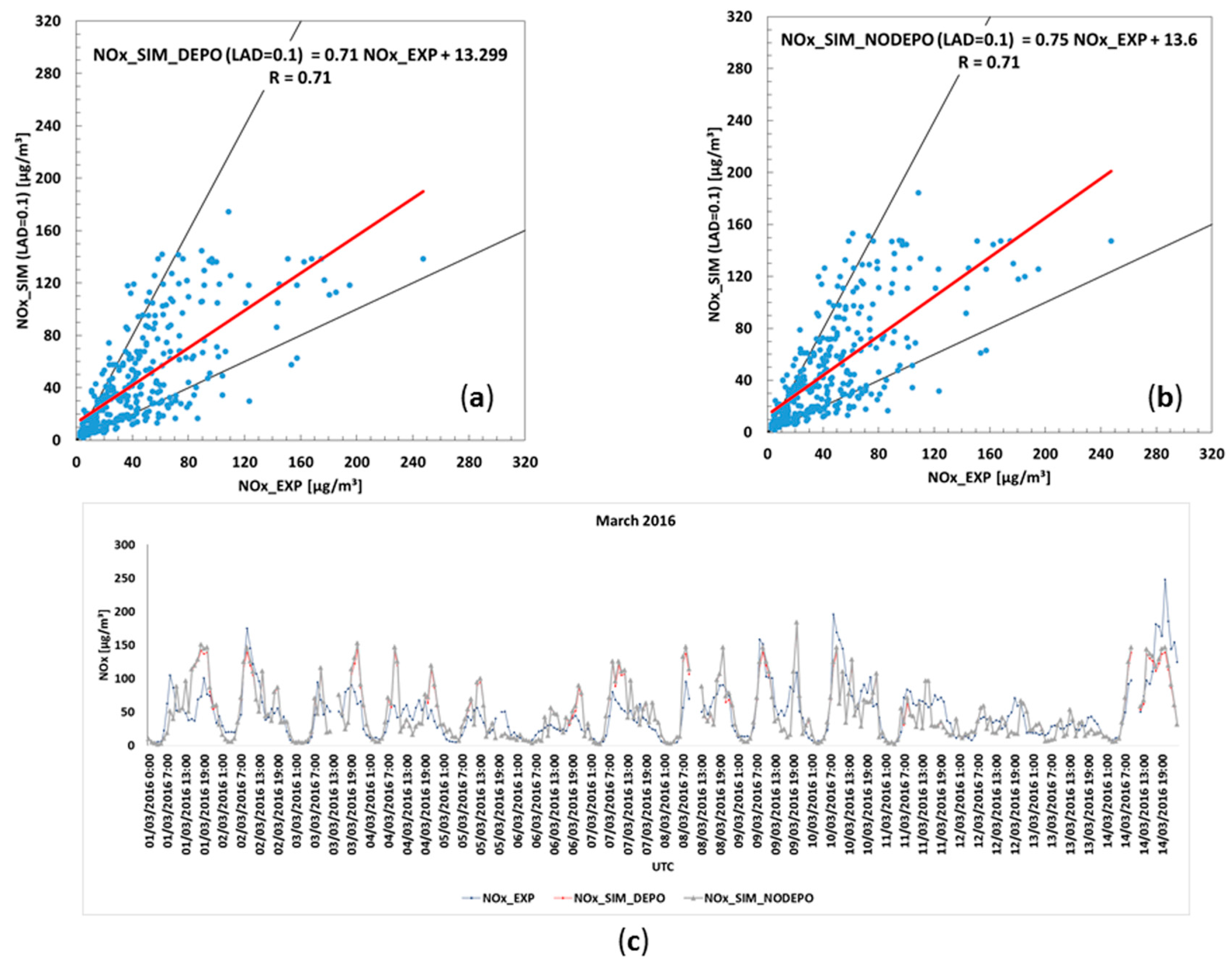
3.2. Current Validation Study

To further get confidence in the use of CFD-RANS, the real scenario of this neighborhood has been here evaluated against data during two weeks in March 2015 (from 1st to 14th) using data from the AQ station. A LAD = 0.1 m²m⁻³ was considered because all trees are deciduous as already mentioned in Section 2.2 [43]. In principle, we are aware that it is necessary to evaluate air quality during large periods of time, but it is usually not affordable to perform unsteady CFD simulations of several days due to large computational costs. For this reason, here the methodology WA CFD-RANS (weighted average CFD-RANS simulations) [42] has been employed: it uses CFD simulations for several wind directions (16 following the wind rose) to compute a time-averaged concentration map, taking into account that the concentration is inversely proportional to wind speed [42]. However, being pollutant deposition considered in this study, this fact is not fulfilled and thus, WA CFD-RANS methodology has been modified as follows:

-

A deposition velocity of 0.01 m s⁻¹ has been considered, which is a high value for NO_x, but still within the range of realistic values [25]. This selection has been done in order to analyze the case where the reduction of concentration by means of vegetation is maximum;

-

Three different ranges of inlet wind speeds were considered to simulate the corresponding scenarios for each wind direction, so 48 simulations have been carried out (

Table 2. Ranges of inlet wind speed at 10 m used in the WA CFD-RANS methodology.

Ranges of Inlet Wind Speed at 10 m	vref/vdep
vref > 4.5 m·s−1	640
2 m·s−1 < vref < 4.5 m·s−1	320
vref < 2 m·s−1	107

);

-

Then, depending on wind speed measured by the meteorological station located close to the neighborhood, at each hour the corresponding simulation was selected and the concentrations were computed.

Results have thus been evaluated against the AQ monitored data (Figure 2). From the figure, small differences between results with and without deposition are observed. The time average difference is 2 µg m⁻³ with a maximum of 11 µg m⁻³ during this time period. Both time series of modelling results have an acceptable correlation with monitored values (R = 0.71). Normalized Mean Square Error (NMSE) and the fraction of predictions within a factor 2 of observation (FAC2) are computed. NMSE is 0.27 and 0.28, and 0.05, and FAC2 is 0.73 and 0.72 for the cases with and without deposition. These values indicate a good agreement between monitored and modelled results with a slightly better fit when deposition is considered and confirm the accuracy of modelling approach for the evaluation of flow and NO_x dispersion within the investigated area in winter period. We are aware that the current methodology has been evaluated for a winter period. During summer when LAD is higher, thermal effects of urban surfaces and trees could be important, and neglecting such effects, as is typically done in many previous studies mainly due to a lack of a common methodology, could introduce more uncertainties in the model results. Furthermore, the evaluation of model simulations with only one measurement point in summer, since there are no other appropriate available data, is not reliable. However, we have confidence at least in the application of the model in cases with higher LAD trees, because it has been validated against CODASC measurements (see Section 3.1). For these reasons, we have focused this paper in winter and we think it can provide useful insights on the use of trees as mitigation strategies.

Considering the time-averaged concentrations in the domain (Figure 3) at 3 m (height of the AQ monitoring station), the effect of deposition in the whole neighborhood is limited and the differences found considering and neglecting deposition are <7 µg m⁻³. In addition, these differences are located only close to the zones characterized by a large amount of vegetation or high concentration of NO_x combined with some trees. For example, there is a difference of 3 µg m⁻³ in the square (dash line (A) in Figure 3b), or there are differences slightly higher in some parts of the avenue North of the domain (dot line (B) in Figure 3b). Then, only in the zones with high amount of vegetation, the differences in time-averaged concentration by including deposition reaches 10%. Therefore, the error in modelling NO_x concentration of considering or neglecting the deposition effect of trees for winter vegetation (LAD = 0.1 m²m⁻³) is low.

From these results, it can be concluded that deposition seems to play a minor role on time- averaged concentration with respect to the aerodynamic effects of trees, even using a high deposition velocity value for NO_x (1 cm s⁻¹). Then, the modelling of this process could be neglected under these conditions.

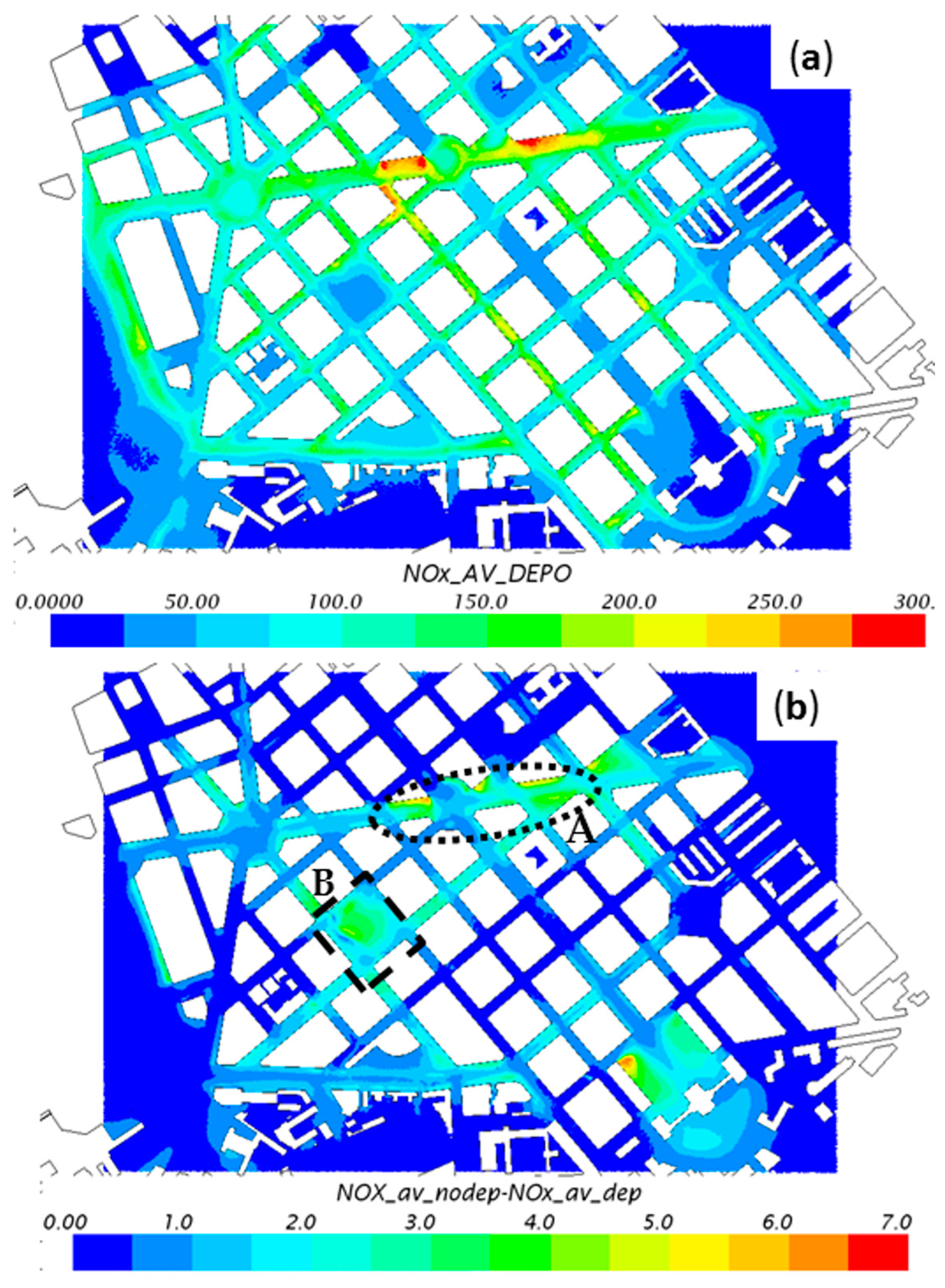
4. Impact of Tree-Foliage on NO_x Concentration: Influence of Deposition and Aerodynamic Effects

In the next sections, the study focuses on conditions of maximum NO_x concentrations. These adverse conditions correspond to the maximum of traffic emissions in the streets during the day (8 a.m.). The inlet meteorological conditions have been taken from the meteorological station located close to the neighborhood. Predominant wind direction (North-West) and average wind speed were computed from these data and used to simulate the typical meteorological conditions at this hour. The impact of tree foliage on urban air quality is thus analyzed, which could provide useful information to urban planners for the selection of appropriate tree species. Then, the objective is to quantify the relative contribution of deposition and aerodynamic effects of vegetation on NO_x concentration in cases with different tree-foliage. LAD = 0.1 and 0.5 m²m⁻³ have in particular been used to model deciduous vegetation from 1st to 14th March 2015 (real cases corresponding to Current-1 scenarios in Table 1) and evergreen vegetation (virtual cases corresponding to Current-2 scenarios in Table 1), respectively.

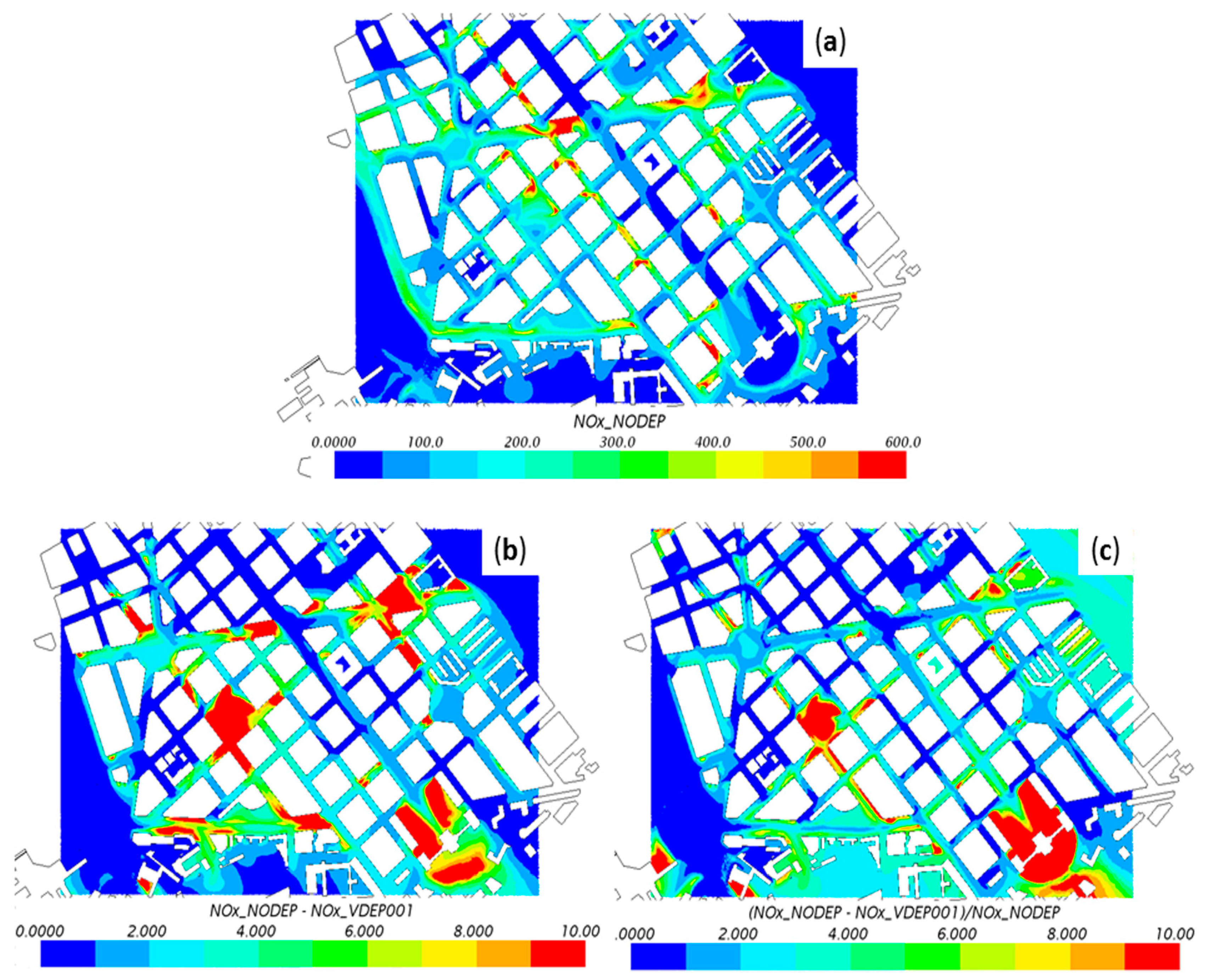
4.1. The Effects of Deposition

Firstly, Current-1 cases are compared to quantify tree deposition for LAD = 0.1 m²m⁻³. Figure 4 shows maps of concentration at 3 m considering vegetation with no deposition (Current-1a) and the absolute and relative differences in a percentage when a deposition velocity of 0.01 m s⁻¹ is used (Current-1a–c). Figure 4b shows decreases of concentration of about 10 µg m⁻³ in some areas close to vegetation and the maximum of reduction is just located within vegetation. Relative percentage differences can reach 10% (Figure 4c). In order to quantify the size of area at 3 m height affected by this concentration reduction, two different criteria have been defined: (1) the zones where the concentration is reduced more than 5 µg m⁻³ (Reduction zone 1); and (2) the zones where the concentration is higher than 50 µg m⁻³ and is reduced more than 5% (Reduction zone 2). Following these criteria, it is found that the Reduction zone 1 and 2 are only 0.9% and 0.7% of the total neighborhood area simulated, respectively. In addition, the overall decrease of spatial-averaged concentrations of the domain with respect to the no-deposition scenario is 0.54%. Deposition thus has no effect on spatial-averaged concentration of the zone. We found that the plan area of vegetation is 13.8% of the domain.

Similar maps are obtained using other deposition velocities. As expected, the reduction of concentration is almost proportional to the deposition velocity.

Table 3. Concentration reduction for vegetation with LAD = 0.1 m²m⁻³ and 3 different deposition velocities (Current-1 scenarios).

Deposition Velocity	Maximum of Reduction (µg m−3)	Maximum of Relative Reduction	Reduction Zone 1 (%)	Reduction Zone 2 (%)	Spatial-Averaged Concentration (µg m−3)	Reduction of Spatial-Averaged Concentration (%)
0.005	6.9	4.5	0.07	0	105.0	0.27
0.01	13.4	8.7	0.9	0.7	104.7	0.54
0.03	35.6	25	7	4	103.7	1.54

shows the reduction parameters for each case. The table shows that, for this type of vegetation, only the effect of pollutant deposition on air quality is not negligible in few zones close to trees.

The increase of tree-foliage induces an increase of pollutant deposition since more surface (leaves) is available for pollutant deposition. In these scenarios (Current-2), evergreen vegetation is modelled with an increase of LAD from 0.1 to 0.5 m²m⁻³. The concentration maps at 3 m for evergreen vegetation with no deposition (Current-2a) and the absolute and relative differences in percentage considering a deposition velocity of 0.01 m s⁻¹ (Current-2a–c) are shown in Figure 5. In these cases, the deposition increases due to vegetation is denser (deposition is proportional to LAD). Then, comparing the results considering and not considering deposition, it can be observed that the decrease of concentration (Current-2a–c) is higher for this LAD (Figure 5b,c). For example, in some zones, the relative reduction can reach 49% and the spatial-averaged concentration of the domain decreases of 2.8% for a deposition velocity of 0.01 m s⁻¹ (Current-2c). Note that the maximum reduction is located within vegetation. In addition, the Reduction zones 1 and 2 increase until 17% and 9.2%, respectively. Results for the other deposition velocities are shown in the

Table 4. Concentration reduction for vegetation with LAD = 0.5 m²m⁻³ and 3 different deposition velocities (Current-2 scenarios).

Deposition Velocity	Maximum of Reduction (µg m−3)	Maximum of Relative Reduction	Reduction Zone 1 (%)	Reduction Zone 2 (%)	Spatial-Averaged Concentration (µg m−3)	Reduction of Spatial-Averaged Concentration (%)
0.005	38	31	8	3.6	111.2	1.5
0.01	66	49	17	9.2	109.7	2.8
0.03	147	74	40	30.5	105.1	6.9

.

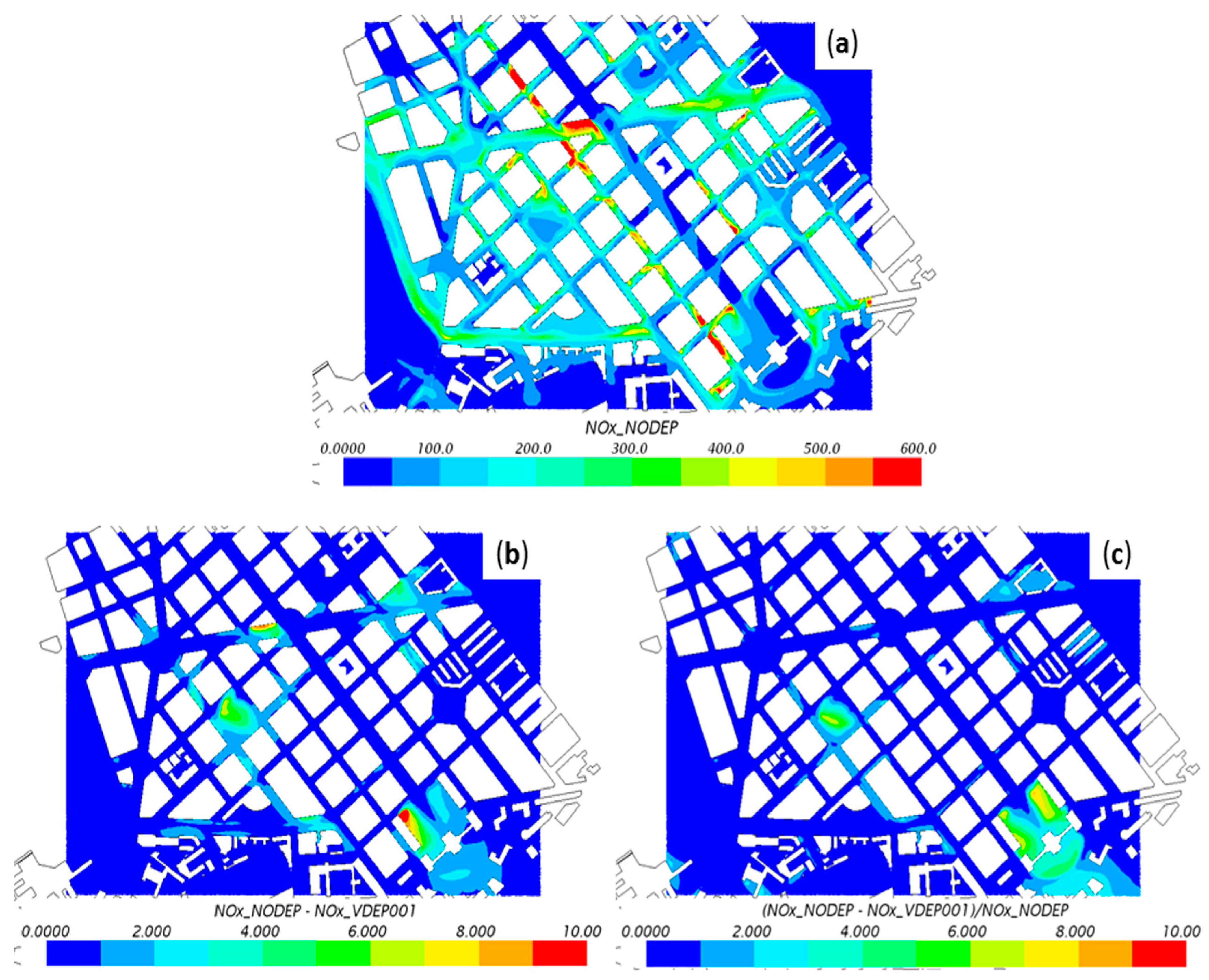
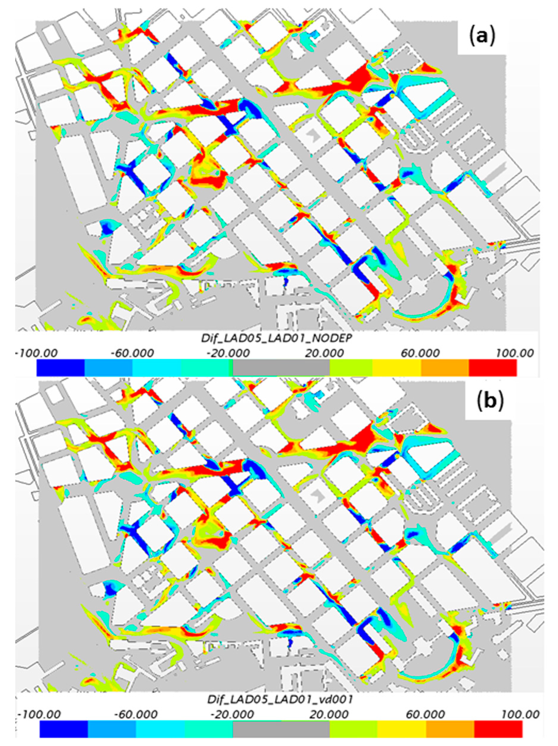
4.2. The Relative Contribution of Aerodynamic and Deposition Effects

The increase of tree-foliage induces not only a greater deposition, but also a greater modification of street ventilation (higher aerodynamic effects). Comparing concentrations obtained for the Current-2 scenarios (LAD = 0.5 m²m⁻³) with those of the Current-1 scenarios (LAD = 0.1 m²m⁻³), it can be noted that the increase of LAD strongly affects the ventilation of the streets inducing different concentration patterns (see Figure 4 and Figure 5). Focusing on aerodynamic effects, differences between Current-2a and Current-1a scenarios are compared (Figure 6a). The figure shows that the concentration increases in some zones or decreases in others and a pedestrian street (street without traffic emissions, see emissions in Figure 1b) is not affected by the increase of LAD. In some other streets, the maximum and minimum of differences are close due to slight displacements of recirculation and stagnation zones. However, the zones where the concentration is higher for LAD = 0.5 m²m⁻³ are wider than the zones where it is reduced. This is also observed considering a deposition velocity 0.01 m s⁻¹ (Figure 6b). For example, the area where the concentration increases of 20 µg m⁻³ or more is 1.81 greater than the area where it decreases of 20 µg m⁻³ or more (2.01 when no deposition is considered), and the average of differences is 5 µg m⁻³ (6.2 µg m⁻³ when no deposition is considered). Moreover, the spatial-averaged concentration increases as LAD increases and the effect of deposition is not enough to cancel out the reduction of ventilation in these cases. Figure 7 shows the spatial-averaged concentrations in the neighborhood for Current-1 and Current-2 scenarios. Here, only for v_dep = 0.03 m s⁻¹ (note that this value is very high and does not seem to be realistic for NO_x) the deposition almost cancels out the effect of ventilation reduction in terms of spatial-averaged concentration. In all cases, the NO_x concentration is clearly higher (1–8%) for Current-2 cases (LAD = 0.5 m²m⁻³) than for Current-1 (LAD = 0.1 m²m⁻³). Thus, it can be concluded that in these cases the aerodynamic effects of vegetation on air pollutant concentration are more important than the deposition.

5. Impact of New Vegetation on NO_x Concentration: Influence of Deposition and Aerodynamic Effects

As in the previous section, the focus is on the adverse conditions characterized by maximum values of NO_x. The effects on concentration due to the introduction of new vegetation in one tree-free street have been investigated. Since the introduction of trees modifies wind flow and changes pollutant distribution within the neighborhood, the main objective of this section is to assess whether the decision of planting new trees could be considered as a mitigation measure of pollutant concentration in this specific study case.

In the investigated neighborhood, there is, in particular, a tree-free street (Tafalla Street, see Figure 8) and virtual scenarios including trees with different foliage (New-1 with LAD = 0.1 m²m⁻³ and New-2 with LAD = 0.5 m²m⁻³) scenarios have been simulated and compared with Current-1 and Current-2 cases (see Table 1). These new trees have modelled with the same features as trees of the parallel street. By introducing such trees, the surface covered by vegetation increases from 13.8 to 14.8% of the domain.

The concentration map of the New-1c scenario is shown in Figure 9. Comparing with results obtained for the Current-1 scenarios (Figure 4), it can be noted that the distribution of pollutant is slightly different. To better illustrate the effects of vegetation, these differences are plotted in Figure 10, which shows that the modification of concentration is a local effect, being the differences of average concentration in the whole neighborhood less than 0.01%. In general, there is an increase of concentration within this street due to the reduction of ventilation. Also, the deposition over these new trees is negligible compared to aerodynamic effects. Only in one area of Tafalla Street, the new trees induce a reduction of pollutant concentration. However, this fact is more due to aerodynamic effects, rather than the deposition. This zone is close to two junctions of streets and one of them is very close to the main avenue at the North. Here, the trees modify the distribution of pollutant increasing in one area and decreasing in other nearby area–it is displacement of the maximum concentration in the same street with negligible average effects. In addition, close to this street (see dash line area in Figure 10), the concentration increases because the presence of trees there induces a recirculation and stagnation zone, as shown in Figure 11. Further, the aerodynamic effects of vegetation seem to be more important than deposition due to the general increases of concentration around Tafalla Street, even though the effects are local. In addition, these effects could affect four streets away from Tafalla Street.

This vegetation configuration is also analyzed for LAD = 0.5 m²m⁻³ (New-2 cases). The concentration map for New-2c case is shown in Figure 12. As shown in the previous section, the effects of vegetation are more intense for higher LAD. However, the differences of average concentration in the whole neighborhood are negligible as for low LAD. In this case, the introduction of new vegetation in Tafalla Street induces more significant modifications in the concentration patterns due to greater drag exerted by new trees (Figure 13). Zones further from Tafalla Street are also affected by these trees. In addition, in the area delimited by dashed line (Figure 13), the concentration also increases due to the air recirculation created by the inclusion of trees (Figure 14).

Results above show that any variation in the distribution of vegetation should be done with caution because the levels of resulting concentrations might change by a modification of the flow also in surrounding areas, and this modification increases with increasing LAD.

6. Summary and Conclusions

In this study, the impact of urban trees has been evaluated in a real neighborhood, which has only been done in few recent studies. A methodology to compute modelled concentration during a long period of time (e.g., several weeks, months, or a year) considering deposition (WA CFD-RANS) was applied and enhanced to account for both the aerodynamic and deposition effects of trees. Modelled results were evaluated with data recorded at an air quality monitoring station. Concentration maps related to adverse conditions (high NO_x concentrations) in winter have been studied in a real case, considering different deposition velocities and for other virtual vegetation scenarios with different tree-foliage and including new trees in one tree-free street. This study can be interpreted as a decision support for urban planners. It is observed that measures which are supposed to indicate the service value of trees could not be used as a general mitigation strategy of pollutant concentration in streets with traffic, since the deposition plays a minor role with respect to aerodynamic effects of trees.

Specifically, the main conclusions achieved from this study are:

-

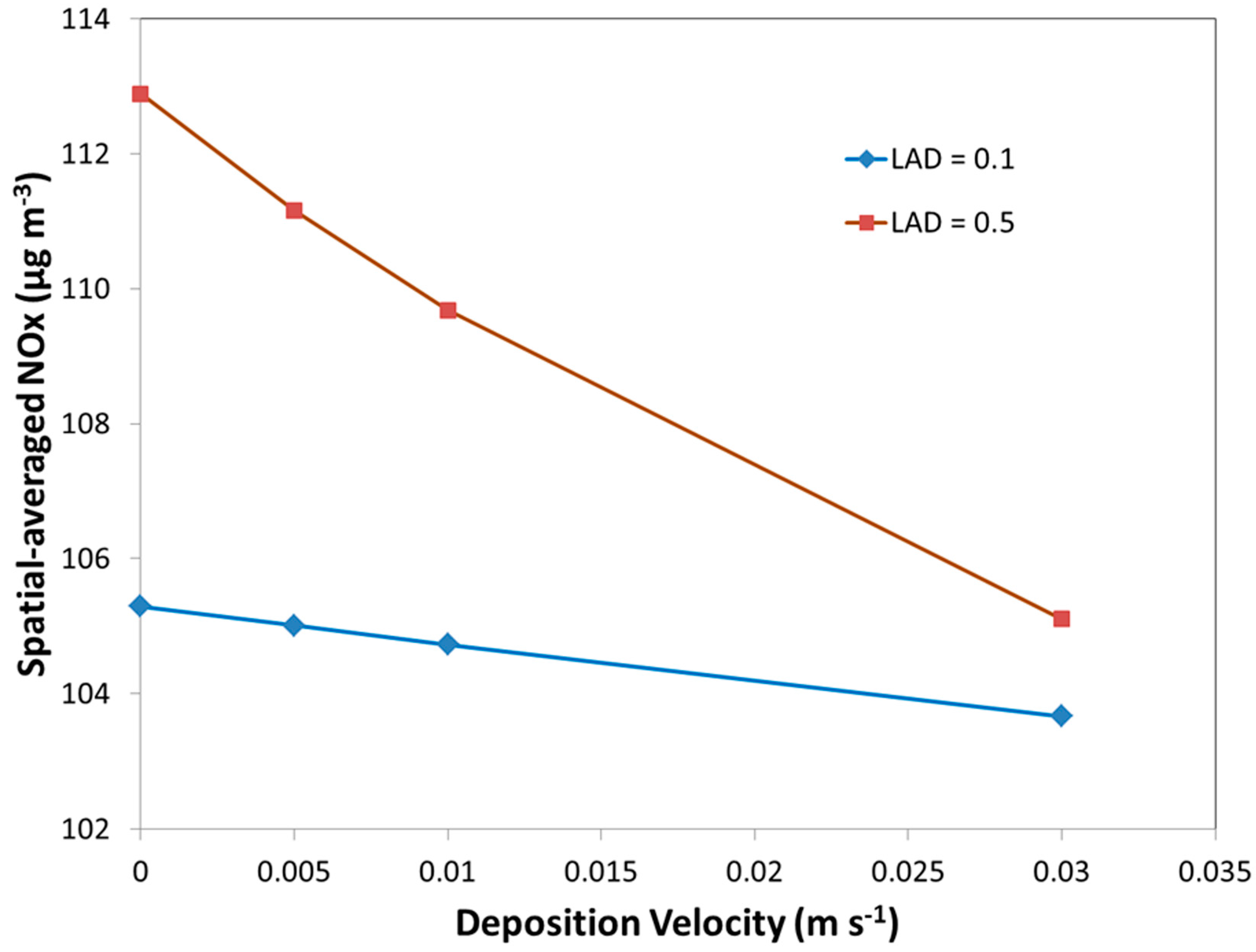
The global decrease of concentration at 3 m in the neighborhood due to deposition is small for cases with low LAD (deciduous). For example, in the real-tree case comparing spatial-averaged concentrations from no deposition simulation with simulation considering a deposition velocity of 0.03 m s⁻¹ (very high deposition velocity), differences of less than 2% are observed. A slightly higher effect (6.9%) is obtained for LAD = 0.5 m²m⁻³; however, deposition effects could be locally higher in certain zones, especially for higher LADs;

-

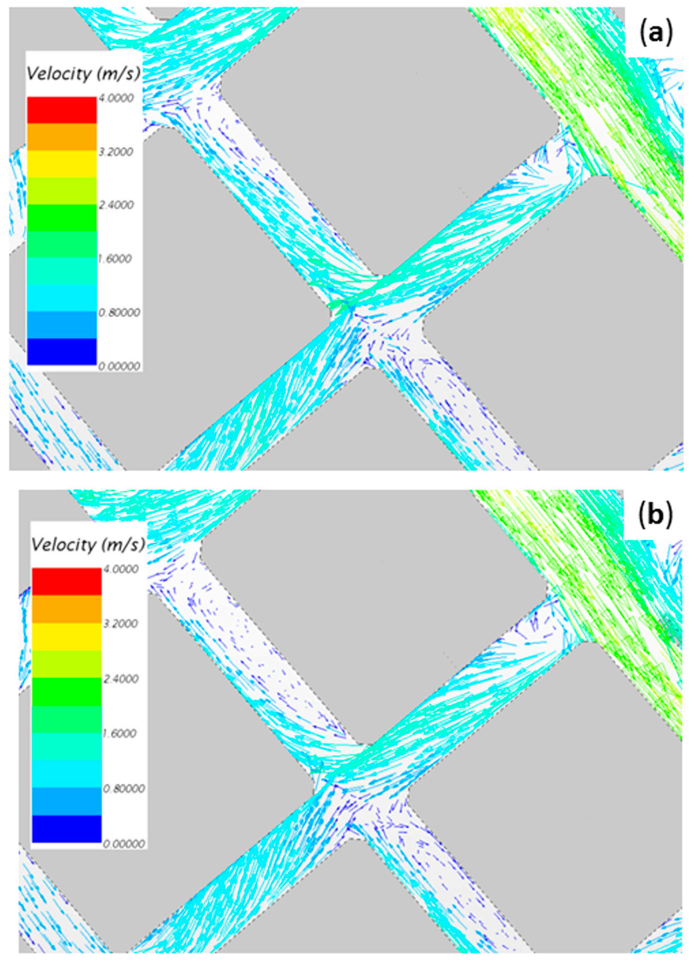
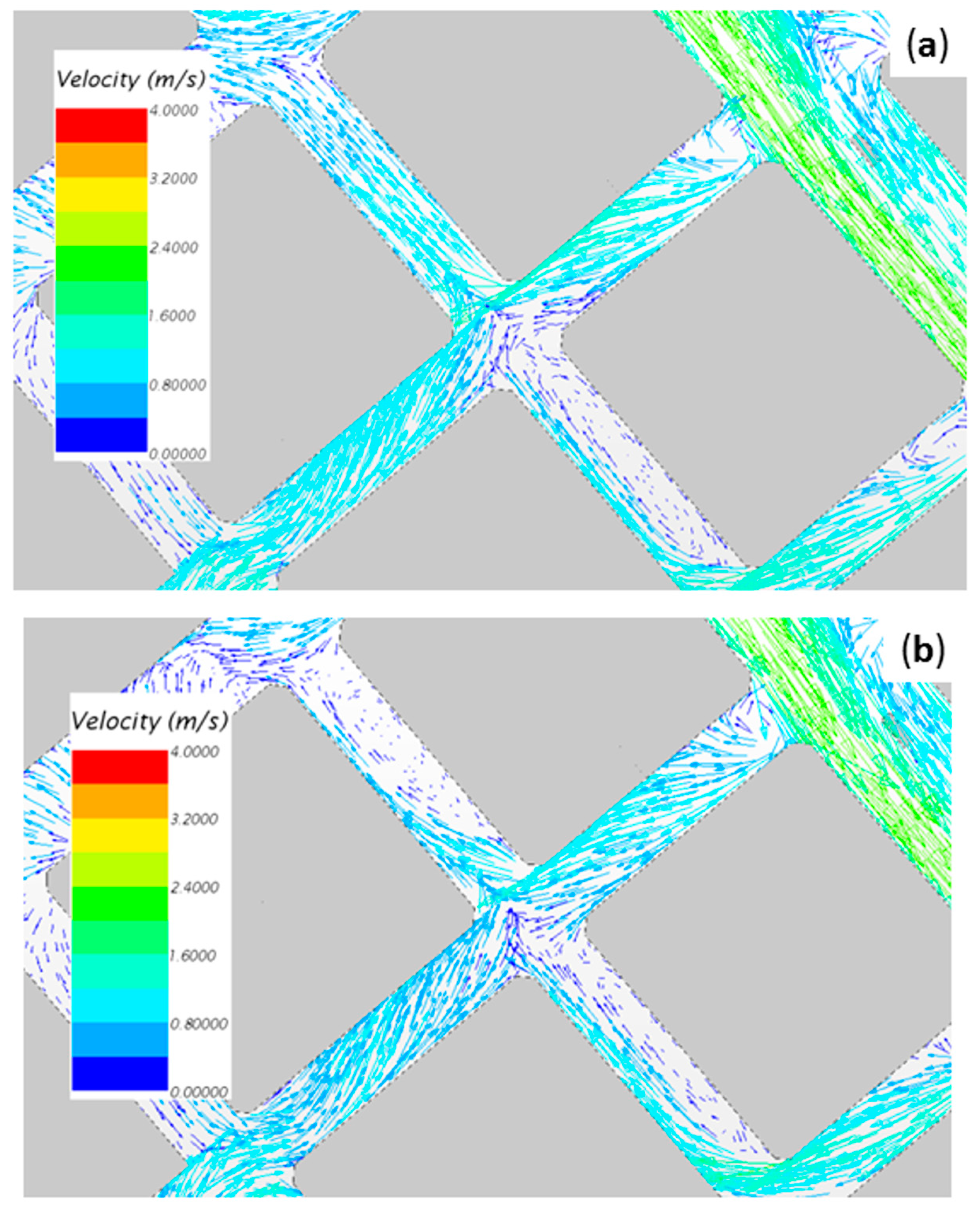
The aerodynamic effects of vegetation induce a general increase of concentration which dominates versus the decreasing of concentration due to deposition. Comparing cases with different LADs, deposition increases with increasing LAD—however spatial-averaged concentrations are always higher for high LADs (dense foliage);

-

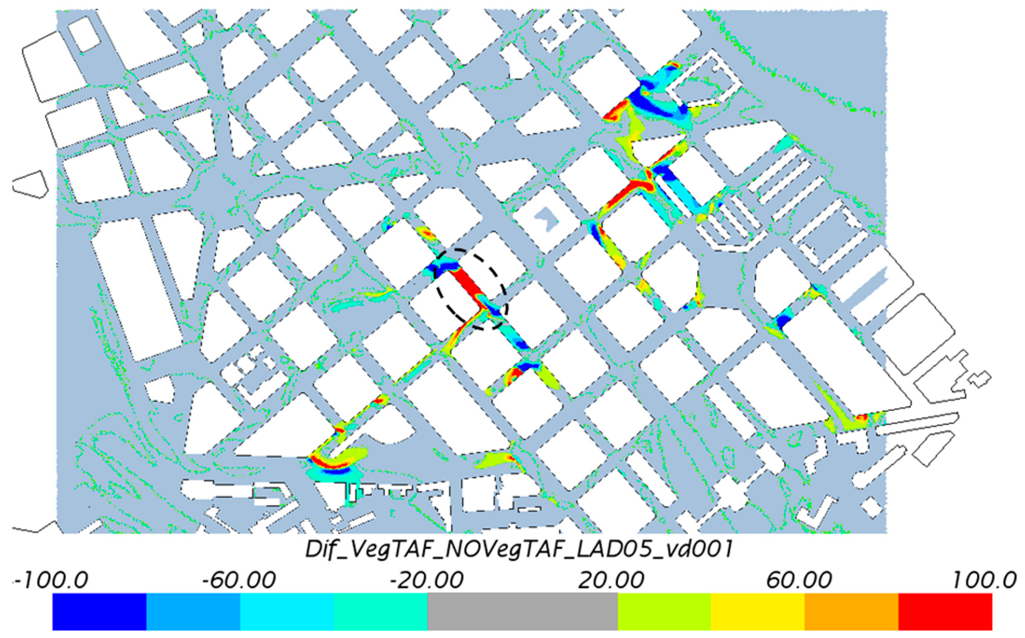
The inclusion of new trees in one street modifies the distribution of pollutant, not only in that street, but also in nearby locations. Global effects in pollutant concentration are small, however, locally differences much greater of 20 µg m⁻³ are found when comparing Current cases with New cases. In some zones, the concentration increases with the new trees, but decreases in others. Also, the use of vegetation as an air pollution reduction strategy within the streets seems to not be appropriate in general, and local studies would be necessary for each particular case to select the suitable location of new vegetation planted.

This work confirms previous findings about the predominance of the aerodynamic effects of vegetation on deposition. In addition, this study has been applied to a complex geometry (real scenario) which is different from idealized cases that are commonly investigated in the literature, since extra turbulence mixing caused by surrounding buildings complicates flow and dispersion within the investigated streets. These conclusions are restricted to the configurations investigated here, but can be extrapolated to other cities with similar street layout and similar tree species, for example, typical Mediterranean cities.

An important assumption made here is to treat vegetation in rows within the streets. This was done due to the absence of individual tree data (geo data or inventory of trees) in this Pamplona neighborhood. Vegetation was thus modelled as rows of trees. In order to take into account the gap between trees, we used a value of LAD for the whole row lower than the LAD corresponding to an individual tree. This approach could locally affect the results, however the general impact of trees is captured by the model. As an example, Buccolieri et al. [55] studied the impact of stand density of trees on pollutant levels and distribution by using wind-tunnel experiments and CFD simulations and no significant impact was found, suggesting that stand density has a minor impact with respect to the street geometry and meteorological conditions. As a future line of research, it would be interesting to carry out more studies about the effect of tree geometry (e.g., considering gap between trees, LAD changing with height, etc.) on pollutant dispersion. Other urban properties such as layout of buildings (e.g., ratio between height of building and width of the street, packing density, distribution of buildings) and the relative location between emissions and trees should be analyzed in each studied district in order to provide information about the appropriate green infrastructure.

In future, more field experimental data are needed to support these modelled results. These new experiments should help the modelling community to improve vegetation modelling in order to gain confidence in CFD modelling as a useful planning tool. In addition, it would be important to investigate the effect of shape and size of tree crowns and improve their representation (and modelling) in CFD models.

References

- Gallagher, J.; Baldauf, R.; Fuller, C.H.; Kumar, P.; Gill, L.W.; McNabola, A. Passive methods for improving air quality in the built environment: A review of porous and solid barriers. Atmos. Environ. 2015, 120, 61–70. [Google Scholar] [CrossRef]
- Livesley, S.J.; McPherson, E.G.; Calfapietra, C. The urban forest and ecosystem services: Impacts on urban water, heat, and pollution cycles at the tree, street, and city scale. J. Environ. Qual. 2016, 45, 119–124. [Google Scholar] [CrossRef] [PubMed]
- Grote, R.; Samson, R.; Alonso, R.; Amorim, J.H.; Cariñanos, P.; Churkina, G.; Fares, S.; Le Thiec, D.; Niinemets, Ü.; Mikkelsen, T.N. Functional traits of urban trees in relation to their air pollution mitigation potential: A holistic discussion. Front. Ecol. Environ. 2016, 14, 543–550. [Google Scholar] [CrossRef]
- Mao, Y.; Wilson, J.D.; Kort, J. Effects of a shelterbelt on road dust dispersion. Atmos. Environ. 2013, 79, 590–598. [Google Scholar] [CrossRef]
- Salmond, J.A.; Williams, D.E.; Laing, G.; Kingham, S.; Dirks, K.; Longley, I.; Henshaw, G.S. The influence of vegetation on the horizontal and vertical distribution of pollutants in a street canyon. Sci. Total Environ. 2013, 443, 287–298. [Google Scholar] [CrossRef] [PubMed]
- Jin, S.; Guo, J.; Wheeler, S.; Kan, L.; Che, S. Evaluation of impacts of trees on PM2.5 dispersion in urban streets. Atmos. Environ. 2014, 99, 277–287. [Google Scholar] [CrossRef]
- Chen, X.; Pei, T.; Zhou, Z.; Teng, M.; He, L.; Luo, M.; Liu, X. Efficiency differences of roadside greenbelts with three configurations in removing coarse particles (PM10): A street scale investigation in Wuhan, China. Urban For. Urban Green. 2015, 14, 354–360. [Google Scholar] [CrossRef]
- Mori, J.; Sæbø, A.; Hanslin, H.M.; Teani, A.; Ferrini, F.; Fini, A.; Burchi, G. Deposition of traffic-related air pollutants on leaves of six evergreen shrub species during a Mediterranean summer season. Urban For. Urban Green. 2015, 14, 264–273. [Google Scholar] [CrossRef]
- Tong, Z.; Whitlow, T.H.; MacRae, P.F.; Landers, A.J.; Harada, Y. Quantifying the effect of vegetation on near-road air quality using brief campaigns. Environ. Pollut. 2015, 201, 141–149. [Google Scholar] [CrossRef] [PubMed]
- Di Sabatino, S.; Buccolieri, R.; Pappaccogli, G.; Leo, L.S. The effects of trees on micrometeorology in a real street canyon: Consequences for local air quality. Int. J. Environ. Pollut. 2015, 58, 100–111. [Google Scholar] [CrossRef]
- Chen, L.; Liu, C.; Zou, R.; Yang, M.; Zhan, Z. Experimental examination of effectiveness of vegetation as bio-filter of particulate matters in the urban environment. Environ. Pollut. 2016, 208, 198–208. [Google Scholar] [CrossRef] [PubMed]
- Hofman, J.; Bartholomeus, H.; Janssen, S.; Calders, K.; Wuyts, K.; Van Wittenberghe, S.; Samson, R. Influence of tree crown characteristics on the local PM10 distribution inside an urban street canyon in Antwerp (Belgium): A model and experimental approach. Urban For. Urban Green. 2016, 20, 265–276. [Google Scholar] [CrossRef]
- Tong, Z.; Whitlow, T.H.; Landers, A.; Flanner, B. A case study of air quality above an urban roof top vegetable farm. Environ. Pollut. 2016, 208, 256–260. [Google Scholar] [CrossRef] [PubMed]
- Gromke, C.; Ruck, B. Pollutant Concentrations in Street Canyons of Different Aspect Ratio with Avenues of Trees for Various Wind Directions. Bound.-Layer Meteorol. 2012, 144, 41–64. [Google Scholar] [CrossRef]
- Huang, C.W.; Lin, M.Y.; Khlystov, A.; Katul, G. The effects of leaf area density variation on the particle collection efficiency in the size range of ultrafine particles (UFP). Environ. Sci. Technol. 2013, 47, 11607–11615. [Google Scholar] [CrossRef] [PubMed]
- Räsänen, J.V.; Holopainen, T.; Joutsensaari, J.; Ndam, C.; Pasanen, P.; Rinnan, A.; Kivimäenpää, M. Effects of species-specific leaf characteristics and reduced water availability on fine particle capture efficiency of trees. Environ. Pollut. 2013, 183, 64–70. [Google Scholar] [CrossRef] [PubMed]
- Gromke, C.; Jamarkattel, N.; Ruck, B. Influence of roadside hedgerows on air quality in urban street canyons. Atmos. Environ. 2016, 139, 75–86. [Google Scholar] [CrossRef]
- Janhäll, S. Review on urban vegetation and particle air pollution—Deposition and dispersion. Atmos. Environ. 2015, 105, 130–137. [Google Scholar] [CrossRef]
- Salmond, J.A.; Tadaki, M.; Vardoulakis, S.; Arbuthnott, K.; Coutts, A.; Demuzere, M.; Dirks, K.N.; Heaviside, C.; Lim, S.; Macintyre, H.; et al. Health and climate related ecosystem services provided by street trees in the urban environment. Environ. Health. 2016, 15 (Suppl. 1), 36. [Google Scholar] [CrossRef] [PubMed] [Green Version]
- Abhijith, K.V.; Kumar, P.; Gallagher, J.; McNabola, A.; Baldauf, R.; Pilla, F.; Broderick, B.; Di Sabatino, S.; Pulvirenti, B. Air pollution abatement performances of green infrastructure in open road and built-up street canyon environments—A review. Atmos. Environ. 2017, 162, 71–86. [Google Scholar] [CrossRef]
- Buccolieri, R.; Salim, S.M.; Leo, L.S.; Di Sabatino, S.; Chan, A.; Ielpo, P.; Gromke, C. Analysis of local scale tree–atmosphere interaction on pollutant concentration in idealized street canyons and application to a real urban junction. Atmos. Environ. 2011, 45, 1702–1713. [Google Scholar] [CrossRef]
- Wania, A.; Bruse, M.; Blond, N.; Weber, C. Analysing the influence of different street vegetation on traffic-induced particle dispersion using microscale simulations. J. Environ. Manag. 2012, 94, 91–101. [Google Scholar] [CrossRef] [PubMed]
- Amorim, J.H.; Rodrigues, V.; Tavares, R.; Valente, J.; Borrego, C. CFD modelling of the aerodynamic effect of trees on urban air pollution dispersion. Sci. Total Environ. 2013, 461, 541–551. [Google Scholar] [CrossRef] [PubMed]
- Santiago, J.L.; Martín, F.; Martilli, A. A computational fluid dynamic modelling approach to assess the representativeness of urban monitoring stations. Sci. Total Environ. 2013, 454–455, 61–72. [Google Scholar] [CrossRef] [PubMed]
- Gromke, C.; Blocken, B. Influence of avenue-trees on air quality at the urban neighborhood scale. Part II: Traffic pollutant concentrations at pedestrian level. Environ. Pollut. 2015, 196, 176–184. [Google Scholar] [CrossRef] [PubMed]
- Jeanjean, A.P.R.; Monks, P.S.; Leigh, R.J. Modelling the effectiveness of urban trees and grass on PM2.5 reduction via dispersion and deposition at a city scale. Atmos. Environ. 2016, 147, 1–10. [Google Scholar] [CrossRef]
- Jeanjean, A.; Buccolieri, R.; Eddy, J.; Monks, P.; Leigh, R. Air quality affected by trees in real street canyons: The case of Marylebone neighbourhood in central London. Urban For. Urban Green. 2017, 22, 41–53. [Google Scholar] [CrossRef]
- Santiago, J.-L.; Martilli, A.; Martin, F. On Dry Deposition Modelling of Atmospheric Pollutants on Vegetation at the Microscale: Application to the Impact of Street Vegetation on Air Quality. Bound.-Layer Meteorol. 2017, 162, 451–474. [Google Scholar] [CrossRef]
- Selmi, W.; Weber, C.; Rivière, E.; Blond, N.; Mehdi, L.; Nowak, D. Air pollution removal by trees in public green spaces in Strasbourg city, France. Urban For. Urban Green. 2016, 17, 192–201. [Google Scholar] [CrossRef]
- Tong, Z.; Baldauf, R.W.; Isakov, V.; Deshmukh, P.; Max Zhang, K. Roadside vegetation barrier designs to mitigate near-road air pollution impacts. Sci. Total Environ. 2016, 541, 920–927. [Google Scholar] [CrossRef] [PubMed]
- Vos, P.E.; Maiheu, B.; Vankerkom, J.; Janssen, S. Improving local air quality in cities: To tree or not to tree? Environ. Pollut. 2013, 183, 113–122. [Google Scholar] [CrossRef] [PubMed]
- Haaland, C.; van den Bosch, C.K. Challenges and strategies for urban green-space planning in cities undergoing densification: A review. Urban For. Urban Green. 2015, 14, 760–771. [Google Scholar] [CrossRef]
- Google Maps®. Available online: https://www.google.es/maps (accessed on 4 May 2017).
- CD-adapco. User Guide STAR-CCM+ Version 7.04. Cd-adapco, 2012. Available online: http://www.cd-adapco.com/products/star-ccm%C2%AE (accessed on 21 July 2017).
- Sanchez, B.; Santiago, J.L.; Martilli, A.; Palacios, M.; Kirchner, F. CFD modeling of reactive pollutant dispersion in simplified urban configurations with different chemical mechanisms. Atmos. Chem. Phys. 2016, 16, 12143–12157. [Google Scholar] [CrossRef]
- Sanchez, B.; Santiago, J.L.; Martilli, A.; Martin, F.; Borge, R.; Quaassdorff, C.; de la Paz, D. Modelling NOx concentrations through CFD-RANS in an urban hot-spot using high resolution traffic emissions and meteorology from a mesoscale model. Atmos. Environ. 2017, 163, 155–165. [Google Scholar] [CrossRef]
- Krayenhoff, E.S.; Santiago, J.L.; Martilli, A.; Christen, A.; Oke, T.R. Parametrization of drag and turbulence for urban neighbourhoods with trees. Bound.-Layer Meteor. 2015, 156, 157–189. [Google Scholar] [CrossRef]
- Sanz, C. A note on k−ε modeling of vegetation canopy air-flows. Bound.-Layer Meteor. 2003, 108, 191–197. [Google Scholar] [CrossRef]
- Google Earth®. Available online: https://www.google.com/intl/es/earth/ (accessed on 4 May 2017).
- Franke, J.; Schlünzen, H.; Carissimo, B. Best Practice Guideline for the CFD Simulation of Flows in the Urban Environment. COST Action 732—Quality assurance and improvement of microscale meteorological models; Distributed by University of Hamburg (Germany), Meteorological Institute: Hamburg, Germany, 2007; ISBN 3-00-018312-4. [Google Scholar]
- Richards, P.; Hoxey, R. Appropriate boundary conditions for computational wind engineering models using the k-turbulence model. J. Wind Eng. Ind. Aerodyn. 1993, 46, 145–153. [Google Scholar] [CrossRef]
- Santiago, J.L.; Borge, R.; Martin, F.; de la Paz, D.; Martilli, A.; Lumbreras, J.; Sanchez, B. Evaluation of a CFD-based approach to estimate pollutant distribution within a real urban canopy by means of passive samplers. Sci. Total Environ. 2017, 576, 46–58. [Google Scholar] [CrossRef] [PubMed]
- Rivas, E.; Santiago, J.L.; Martin, F.; Sánchez, B.; Martilli, A. CFD study of induced effects of trees on air quality in a neighborhood of Pamplona. 10th International Conference on Air Quality—Science and Application, Milan, Italy, 14–18 March 2016; Available online: https://drive.google.com/drive/folders/0B2iFZ3L-H5pRazh6QjlBWGVWcHc (accessed on 3 March 2017).
- Lalic, B.; Mihailovic, D.T. An empirical relation describing leaf-area density inside the forest for environmental modeling. J. Appl. Meteor. 2004, 43, 641–645. [Google Scholar] [CrossRef]
- Brunet, Y.; Finnigan, J.J.; Raupach, M.R. A wind tunnel study of air flow in waving wheat: Single-point velocity statistics. Bound.-Layer Meteor. 1994, 70, 95–132. [Google Scholar] [CrossRef]
- Raupach, M.R.; Bradley, E.F.; Ghadiri, H. Wind Tunnel Investigation Into the Aerodynamic Effect of Forest Clearing on the Nesting of Abbott’s Booby on Christmas Island; Internal report; CSIRO Centre for Environmental Mechanics: Canberra, Australia, 1987. [Google Scholar]
- Foudhil, H.; Brunet, Y.; Caltagirone, J.P. A Fine-Scale k−ε Model for Atmospheric Flow over Heterogeneous Landscapes. Environ. Fluid Mech. 2005, 5, 247–265. [Google Scholar] [CrossRef]
- Dupont, S.; Brunet, Y. Edge flow and canopy structure: A large-eddy simulation study. Bound.-Layer Meteor. 2008, 126, 51–71. [Google Scholar] [CrossRef]
- Gromke, C.; Ruck, B. Influence of trees on the dispersion of pollutants in an urban street canyon-experimental investigation of the flow and concentration field. Atmos. Environ. 2007, 41, 3287–3302. [Google Scholar] [CrossRef]
- Gromke, C.; Ruck, B. On the impact of trees on dispersion processes of traffic emissions in street canyons. Bound.-Layer Meteor. 2009, 131, 19–34. [Google Scholar] [CrossRef]
- Gromke, C.; Buccolieri, R.; Di Sabatino, S.; Ruck, B. Dispersion study in a street canyon with tree planting by means of wind tunnel and numerical investigations—Evaluation of CFD data with experimental data. Atmos. Environ. 2008, 42, 8640–8650. [Google Scholar] [CrossRef]
- Balczó, M.; Gromke, C.; Ruck, B. Numerical modeling of flow and pollutant dispersion in street canyons with tree planting. Meteorologische. Zeitschrift. 2009, 18, 197–206. [Google Scholar] [CrossRef]
- Vranckx, S.; Vos, P.; Maiheu, B.; Janssen, S. Impact of trees on pollutant dispersion in street canyons: A numerical study of the annual average effects in Antwerp, Belgium. Sci. Total Environ. 2015, 532, 474–483. [Google Scholar] [CrossRef] [PubMed]
- Moonen, P.; Gromke, C.; Dorer, V. Performance assessment of large eddy simulation (LES) for modelling dispersion in an urban street canyon with tree planting. Atmos. Environ. 2013, 75, 66–76. [Google Scholar] [CrossRef]
- Buccolieri, R.; Gromke, C.; Di Sabatino, S.; Ruck, B. Aerodynamic effects of trees on pollutant concentration in street canyon. Sci. Total Environ. 2009, 407, 5247–5256. [Google Scholar] [CrossRef] [PubMed]