
Future Changes in Global Precipitation Projected by the Atmospheric Model MRI-AGCM3.2H with a 60-km Size

Climate Research Department, Meteorological Research Institute, 1-1, Nagamine, Tsukuba, Ibaraki 305-0052, Japan
Atmosphere 2017, 8(5), 93; https://doi.org/10.3390/atmos8050093
Submission received: 10 March 2017
/
Revised: 15 May 2017
/
Accepted: 17 May 2017
/
Published: 21 May 2017
(This article belongs to the Special Issue Global Precipitation with Climate Change)
Abstract
:We conducted global warming projections using the Meteorological Research Institute-Atmospheric General Circulation Model Version 3.2 with a 60-km grid size (MRI-AGCM3.2H). For the present-day climate of 21 years from 1983 through 2003, the model was forced with observed historical sea surface temperature (SST). For the future climate of 21 years from 2079–2099, the model was forced with future SST projected by conventional couple models. Twelve-member ensemble simulations for three different cumulus convection schemes and four different SST distributions were conducted to evaluate the uncertainty of projection. Annual average precipitation will increase over the equatorial regions and decrease over the subtropical regions. The future precipitation changes are generally sensitive to the cumulus convection scheme, but changes are influenced by the SST over the some regions of the Pacific Ocean. The precipitation efficiency defined as precipitation change per 1° surface air temperature warming is evaluated. The global average of precipitation efficiency for annual average precipitation was less than the maximum value expected by thermodynamical theory, indicating that dynamical atmospheric circulation is acting to reduce the conversion efficiency from water vapor to precipitation. The precipitation efficiency by heavy precipitation is larger than that by moderate and weak precipitation.
1. Introduction
Uncertainty in future climate change projected by climate models originates from four main factors: emission scenario, model structure, internal natural variability and initial condition and external forcing and boundary condition [1]. For a given specific emission scenario, uncertainty of future projection is often evaluated as a spread of responses by multiple models. A single model can be used to estimate the spread of internal natural variability if it is integrated from multiple initial conditions. The spread of responses by a single model can be also estimated by implementing multiple versions of physical processes into the model [2].
It is natural to assume that future projection by models with higher reproducibility of observed climate is more reliable than projections by models with lower reproducibility. In principle, the reproducibility of precipitation climatology improves when we use a model with higher horizontal resolution. Studies by [3,4,5] (Table S1) have revealed that the realistic reproduction of summertime precipitation over East Asia requires an atmospheric model with higher horizontal resolution. Therefore, we have been conducting a series of global warming projection experiments using the Meteorological Research Institute-Atmospheric General Circulation Model Version 3 (MRI-AGCM3) with 20-km and 60-km grid sizes [3,4,6,7,8,9,10,11,12,13,14] (Table S1). These models have relatively higher horizontal resolution compared with global atmospheric models generally used in climate variability studies.
Since the MRI-AGCM3 model has only the atmosphere and lacks the oceans, we have to specify sea surface temperature (SST) to conduct the global warming projection. We adopted a ‘time-slice experiment’ [15] where the model was forced by prescribed external boundary conditions and forcing. For the present-day climate, observed SSTs were given to the model. This kind of model experiment is conventionally called the Atmospheric Model Intercomparison Project (AMIP)-type simulation, which is a standard method to evaluate the performance of atmospheric models. For the future climate, future SSTs projected by the conventional atmosphere-ocean general circulation model (AOGCMs) are given to the model.
One of the striking advantages of time-slice experiment is that we can increase the horizontal resolution of atmospheric part, because we can save computer resources allocated for the ocean part. Another advantage is that the present-day climatology simulated by an atmospheric model tends to be better than that by an AOGCM, because SST prescribed in the present-day climatology is observation. Errors in SST observation are generally smaller than those simulated by AOGCMs. SST simulated by AOGCM has inevitable errors leading to the distortion of model climatology.
On the other hand, the disadvantage of the time-slice experiment is the lack of air-sea interaction. Future change in the Indian monsoon is influenced by the SST-convection relationship, which would be erroneously distorted if SST feedback from the atmosphere is not taken into account [16]. Tropical cyclone simulated by the atmospheric model tends to show overestimation of intensity [17] and erroneous northward shift of the existence area in mid-latitudes [18], owing to the lack of cooling by mixing of the ocean surface layer.
Despite this weakness in the time-slice experiment, we selected the option to use the higher horizontal resolution version of the atmospheric global model, which enables us to project the small spatial scale structure of future climate change without any dynamical downscaling using regional climate models. Moreover, we are collaborating with scientists investigating the impact of global warming in the fields of natural disaster prevention, water resource management, agriculture and irrigation. Some of their tools, such as the river discharge model and the flood analysis model, require very high horizontal resolution forcing as input data. This is another reason to introduce a higher horizontal resolution model by the time-slice experiment to meet the requirements of impact assessment scientists.
Simulated precipitation change by the atmospheric model is sensitive to prescribed SST [19]. The dependence of precipitation change on SST was investigated using predicted future SST by some individual AOGCMs participating in the third phase of the Coupled Model Intercomparison Project (CMIP3), as well as the SST of the multi-model ensemble (MME) mean of the CMIP3 AOGCMs [6,7,8,9] (Table S1).
Simulated precipitation change by the atmospheric model is also susceptible to physical processes, such as the cumulus convection scheme implemented in the models. Using the MRI-AGCM3.2S (20 km) and 3.2H (60 km), [9] have conducted a set of ensemble simulations for three different cumulus convection schemes and four different SSTs obtained from the cluster analysis of 18 CMIP3 AOGCMs. They found that the uncertainty of precipitation over the southern part of Asia originates in the difference among cumulus convection schemes, while that over the Maritime Continent (MC) is caused by the difference among SSTs. The dependence of precipitation change on SST was further investigated using future SSTs obtained from the fifth phase of the Coupled Model Intercomparison Project (CMIP5) AOGCMs [11,12,13,14] (Table S1). However, the dependence of precipitation change on the cumulus convection scheme has not yet been fully examined using future SSTs of CMIP5 AOGCMs.
The purpose of this study is to answer the following questions. Firstly, do our models globally perform better than the atmospheric models of other institutions with respect to annual average precipitation, as well as extreme precipitation events? Secondly, how will precipitation change globally with respect to annual average precipitation, as well as extreme precipitation events? Thirdly, how large is the uncertainty of future change? Simulated precipitation by the atmospheric model is apparently sensitive to SST and the cumulus convection scheme. The works in [9,14] have quantitatively evaluated the relative contributions of SST and cumulus convection to the uncertainty of future precipitation change, but their target regions were limited to Asia. Therefore, we need to extend the target region to the whole globe in order to get the big picture of precipitation change from the global perspective. Fourthly, how will precipitation change globally in response to the increase of surface air temperature? In global warming projections, models consistently project a global precipitation increase that is slower than the increase in moisture expected from thermodynamic theoretical estimate [20,21]. We will investigate how the conversion rate of precipitation from water vapor depends on the metrics of precipitation, the cumulus convection scheme and SST.
2. Models and Experimental Design
2.1. The Global Atmospheric Model
The global atmospheric model used in this study is the MRI-AGCM3.2H. This model was cooperatively developed by the Japan Meteorological Agency (JMA) and the MRI [22]. The horizontal grid size of the model is 60 km. Hereafter, we call this model as the 60-km model in this paper. The model has 60 levels reaching to 0.01 hPa top equivalent to an altitude of approximately 80 km. We also used the same version with different horizontal resolution models of the MRI-AGCM3.2S (20 km) and the MRI-AGCM3.2L (180 km) in order to compare the reproducibility of present-day climatology (Table S2).
As for the cumulus convection scheme, we implemented the “Yoshimura scheme” (YS; [23]) which is modified from the Tiedtke scheme [24]. Simulated precipitation by models largely depends on the kind of cumulus convection scheme implemented in the model. Therefore, in order to evaluate the sensitivity of simulated precipitation on the cumulus convection scheme, we further utilized the Arakawa–Schubert (AS) scheme [25] and the Kain–Fritsch (KF) scheme [26], as well as the Yoshimura scheme. These versions of the models were already used for ensemble simulations in previous studies that analyzed future changes in precipitation over Asia [9,10,14].
The Tiedtke, YS and AS schemes are all categorized as classical mass-flux type cumulus schemes. In the Tiedtke scheme, only a single convective updraft is calculated in a single grid point, but is represented as a more detailed entraining and detraining plume. In the AS scheme, on the other hand, multiple convective updrafts with different heights are explicitly calculated within a single grid cell, although each updraft is a more simplified entraining plume. YS can be regarded as a kind of hybrid of the Tiedtke and AS schemes. YS represents all top-level cumulus plumes by interpolating two convective updrafts with maximum and minimum rates of turbulent entrainment and detrainment [27]. YS performs better than the AS scheme in simulating precipitation in the tropics [22] and summer precipitation over East Asia [5]. Because the AS scheme was the default convection scheme for the MRI-AGCM3.0 and 3.1 models, an option for choosing the AS scheme was kept in the MRI-AGCM3.2. The KF scheme was originally developed to simulate the mesoscale convective system (MCS) in mid-latitudes. The KF scheme is based on a one-dimensional cloud model in which the exchange of mass between cloud and environment is modulated through entrainment and detrainment. Since the KF scheme well simulates MCSs, it is implemented in the operational regional model of the JMA. Therefore, we also included the KF scheme in the options of the convection scheme in the MRI-AGCM3.2.
2.2. Sea Surface Temperature and Sea Ice
We adopted a time-slice experiment [15] where the 60-km model was forced by prescribed external boundary conditions and forcing. For the present-day climate from the year 1983–2003 (21 years), we integrated the model giving the observed historical sea surface temperature (SST) and observed sea ice concentration provided by the Hadley Centre sea ice and sea surface temperature data set version 1 (HadISST1) [28].
For the future climate from year 2079–2099 (21 years), the boundary SST data were constructed by combining three components: (i) future change in the MME mean of SST projected by the CMIP5 multi-model model (28 models) dataset; (ii) the linear trend in the MME mean of SST projected by the CMIP5 multi-model dataset; and (iii) the detrended interannual observed SST anomalies for the period from year 1979–2003. Future change in the MME mean of SST was taken from the difference between the historical experiments and the future simulation. We integrated the model under the Representative Concentration Pathway (RCP) 8.5 emission scenario [29] for the future climate. Future sea ice concentration was obtained in a similar manner. For further details, refer to [30].
Considering that the response of atmospheric models is intrinsically susceptible to the SST prescribed, we assessed the dependence of future precipitation change on the geographical distribution of SST. For this purpose, we have separated 28 CMIP5 models into three groups with the clustering analysis based on the future change in annual mean SST projected by CMIP5 models over the tropics (Figure 1a–d). Figure 1e depicts the deviation of Cluster 1 from the average of all models (C0; Figure 1a). Cluster 1 (C1; Figure 1e) is distinguished by larger warming in the Southern Hemisphere as compared to the Northern Hemisphere; Cluster 2 (C2; Figure 1f) is characterized by large warming in the central Pacific in the tropics; Cluster 3 (C3; Figure 1g) is distinguished by large warming around Japan. The future sea ice concentration was calculated according to the clustering of SST. For more details, see [31]. With these four different SST distributions, as well as three different cumulus convection schemes, we can evaluate the spread of the model response, which can be interpreted as the kind of reliability information on future precipitation change.
2.3. Other External Forcings
Observed historical concentrations of greenhouse gases (GHG) such as carbon dioxide and methane were given for the present-day climate simulations. The RCP8.5 emission scenario was applied to the future climate simulations. We used three-dimensional natural and anthropogenic aerosol distributions simulated by the MRI-Earth System Model (MRI-ESM; [27]) based on historical and the Special Report on Emission Scenario (SRES) A1B scenario [32] aerosol emission data. We included aerosols erupted only from Mt. Pinatubo in the year 1991. The three-dimensional distributions of stratospheric ozone calculated by the MRI-Chemical Transport Model (CTM) (MRI-CTM; [33]) based on historical and A1B scenario aerosol emission data were prescribed. Aerosol and stratospheric ozone distributions simulated by the MRI-ESM and MRI-CTM assuming the RCP8.5 scenario were not available at the time when we started a set of global warming projections in this study. Table 1 summarizes the experimental designs and definitions of the simulation names.
3. Present-Day Climate
3.1. Observation for Model Verification
To validate the model, we used the One-Degree Daily data (1dd) of the Global Precipitation Climatology Project (GPCP) v1.2 compiled by [34] from 1997–2008 (12 years). The horizontal resolution of this dataset is 1.0° in longitude and latitude, corresponding to a grid spacing of roughly 90 km at 35° N. The quantitative model performances were evaluated against GPCP 1dd data. Since the 60-km models have relatively higher horizontal resolution, we need observational data with higher horizontal resolution for verification. However, the GPCP 1dd data do not cover the whole target period of simulations from 1983–2003. Pentad and monthly data are calculated from daily data. In the verification, model data were interpolated to the location of grid points of the GPCP 1dd data.
Observational data themselves have uncertainty of observation so that model skill depends on the selection of observational data [35]. The pentad and monthly data of GPCP v2.2 provided by [36] are also utilized from 1983–2003 (21 years). These data cover the whole target period of simulations from 1983–2003. The horizontal resolution of this dataset is 2.5° in longitude and latitude, corresponding to a grid spacing of roughly 210 km at 35° N.
Further, the pentad and monthly data of the Climate Prediction Center Merged Analysis of Precipitation (CMAP) v1201 compiled by [37] are used from 1983–2003 (21 years). The horizontal resolution of this dataset is 2.5° in longitude and latitude, which is the same as GPCP v2.2. Moreover, we used the Tropical Rainfall Measuring Mission (TRMM) 3B43 compiled by [38] from 1998–2010 (13 years). The horizontal resolution is 0.25° in longitude and latitude, corresponding to a grid spacing of about 25 km at 35° N. However, regional coverage is restricted to a global belt extending from 50° S–50° N. Table 2 summarizes the observations used for verification.
3.2. Global Distribution of Precipitation
The global distributions of annual average precipitation (PAV) simulated by the models are compared with observations (Figure 2). In the observation of GPCP 1dd (Figure 2a), the region of large precipitation extends over the Equator in the Indian Ocean, the Pacific Ocean, the Atlantic Ocean and the Amazon in South America. Furthermore, precipitation is large over the South Pacific Convergence Zone (SPCZ), which spreads over the MC and Papua New Guinea. In middle and high latitudes in the Northern Hemisphere, precipitation shows moderate maxima over the North West Pacific Ocean and the North West Atlantic Ocean. These regions correspond to the location of storm tracks owing to the frequent passage of extratropical cyclones. Convective rainfall driven by the underlying warm western boundary ocean currents also contributes in these regions [39]. The large-scale geographical distributions of precipitation by other observations (Figure 2b–d) are approximately similar to that of GPCP 1dd (Figure 2a). Local maximum of precipitation over the MC is larger in Figure 2c,d than in Figure 2a, while precipitation over the MC is smaller in Figure 2b than in Figure 2a (also see Figure S1).
The 60-km models well reproduce the large-scale distribution of precipitation (Figure 2e–g), but the precipitation over the maritime continent and the SPCZ is overestimated compared with observations (Figure 2a–d). The MME mean of the CMIP5 atmospheric models’ AMIP runs (Table S1) forced with a similar SST as the 60-km models shows also a realistic precipitation distribution (Figure 2h). The grid size at 35° N of CMIP5 atmospheric models ranges from 28 km–342 km with an average of 171.5 km and a median 171 km, which is larger than that of the 60-km model (last column in Table S2). The 60-km model with the KF scheme (Figure 2g) shows the largest precipitation over the MC compared with the other models (Figure 2e,f,h and Figure S2), which can be also confirmed in Figure S2f.
In terms of model biases against GPCP 1dd v1.2 (Figure 2i–l), all models show excessive precipitation over the MC and the central tropical Pacific Ocean.
3.3. Taylor Diagram
In order quantify the skill of models, we introduced the skill score S proposed by [40] against the GPCP 1dd data (Figure 2a). S is defined by:
where R is the spatial correlation coefficient between observation and simulation, σ is the spatial standard deviation of the simulation divided by that of the observations and R0 is the maximum correlation attainable. Here, we assumed that R0 = 1. S evaluates the spatial correlation coefficient, as well as the spatial standard deviation. S approaches unity in a perfect simulation.
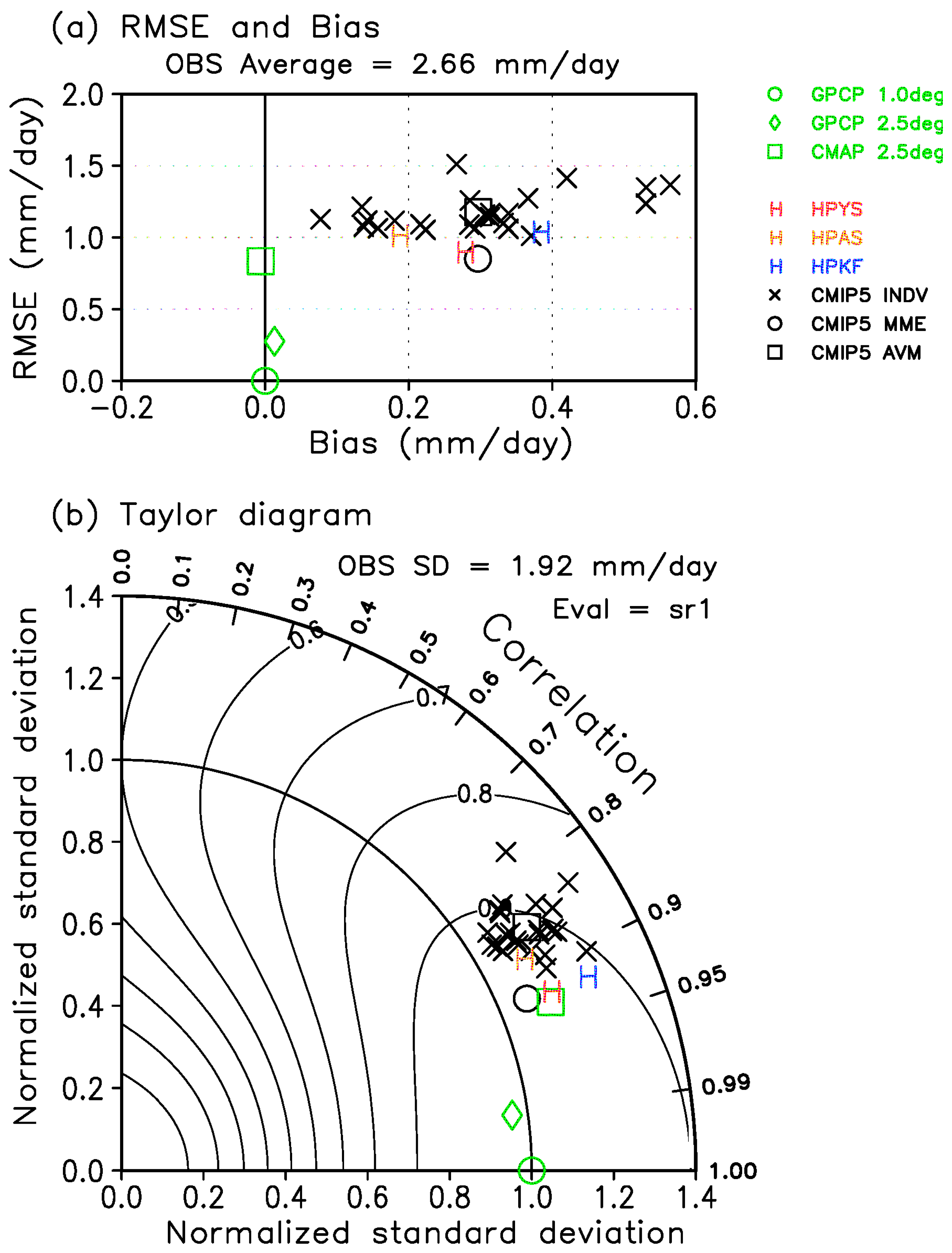
Figure 3b displays the Taylor diagram [40] of S for the 60-km and CMIP5 atmospheric models with respect to PAV. Although S is widely used to verify model performance in many climate modelling studies, we must recognize that S cannot evaluate model bias because this method deals with deviation from the mean value of the target domain both for observation and simulations. Therefore, we also plotted the bias and root mean square error (RMSE) in Figure 3a. The target region is the global domain (Figure 2). In the Taylor diagram (Figure 3b), the radial distance from the origin is proportional to the standard deviation of a simulated spatial pattern normalized by the observed standard deviation. The spatial correlation coefficient between the observed and simulated fields is given by the angle from the Y-axis. The skills of the GPCP 2.5° data and CMAP 2.5° data against the GPCP 1dd data were also plotted to estimate the uncertainty of observations. This uncertainty originates from the differences of averaged period, horizontal resolution, original source of data and retrieval method. The difference among observations (green marks) is relatively small compared with the difference among all models (Figure 2a,b).
Figure 3a shows that all of the 60-km and all of the 24 CMIP5 models have positive biases mainly originating from overestimation of precipitation over the MC and the SPCZ. The RMSEs of the 60-km models (character H) are smaller than or comparable to those of the CMIP5 models (black X).
We calculated the average skill of the individual CMIP5 models (AVM, black square), as well as the skill of the spatial distribution of precipitation constructed from the MME mean (black circle) of CMIP5 models. In the calculation of the AVM, we first evaluated the skill of the geographical distribution of precipitation simulated by individual models, and then, we averaged all 24 skills. In the case of linear skill measures, such as average and bias, the MME mean is identical to the AVM. In the case of nonlinear skill measures, such as RMSE, the correlation coefficient and Taylor skill score S, the MME mean and the AVM differ. In Figure 3a, the RMSE of MME (black circle) is smaller than that of the AVM (black square). This is consistent with previous findings that the MME mean average can be expected to outperform individual models in climate simulations [41,42,43]. The 60-km model with YS (red H) shows the smallest RMSE of all models.
In the Taylor diagram (Figure 3b), the Taylor skill scores S (contour plot) of the 60-km models (H) are also closer to the GPCP 1dd observation (green circle) than those of the CMIP5 models (black X). The MME mean (black circle) is closer to the observation (green circle) than the AVM (black square) as in Figure 3a. All of the models are plotted outside the quadrant of radius one. This means that the simulated precipitation distribution has larger spatial variability than observation. The spatial variability of the 60-km models is nearly comparable to that of the CMIP5 models, but the spatial pattern simulated by the 60-km models is better than that by most CMIP5 models. The 60-km model with YS (red H) is the closest to the observation (green circle) of all models.
In summary, the 60-km models perform better than or equal to the CMIP5 models in terms of bias, RMSE, spatial pattern and Taylor skill score S, although the spatial variability of the 60-km model is almost equivalent to that of the CMIP5 models.
3.4. Extreme Precipitation Events
We adopted four extreme precipitation indices (Table 3) from those proposed by [44]. PAV is also included for comparison. These are indices measuring precipitation intensity, except for consecutive dry days (CDD), which is a measure for dryness and the possibility of drought. These indices are based on annual statistics. The Simple Daily precipitation Intensity Index (SDII) is widely adopted in model studies, such as [45]. The maximum 5-day precipitation total (R5d) is a relevant measure to estimate the possibility of natural disasters, such as flood and land slide. The indices SDII, R5d and CDD are also adopted in Figure 9.37 of [46]. In the previous studies dealing with extreme precipitation events, notations Rx5day and Rx1day are widely used to define R5d and The maximum 1-day precipitation total (PMAX), respectively.
Figure 4 compares the spatial correlation coefficients of the 60-km models against GPCP 1dd with those of CMIP5 models with respect to the global distributions of extreme precipitation indices (Table 3). In the case of PAV, the skills of the 60-km models are higher than the average skill of CMIP5 models (AVM, green line). The skills of the 60-km models with YS (red line) and with the KF scheme (blue line) are even higher than the MME mean of CMIP5 models (green circle). In the case of SDII, R5d, PMAX and CDD, the skills of the 60-km models are higher or comparable to those of CMIP5 models. However, the models with the AS scheme show the lowest correlation coefficient among the 60-km models. This is due to the under-estimation of precipitation intensity by the 60-km model with the AS scheme compared with models with the other cumulus scheme. See Figure S3 for the R5d case.
In terms of RMSE, the skills of the 60-km models are also higher or comparable to those of CMIP5 models, except for CDD (Figure S4). The 60-km models have relatively larger positive bias of CDD compared to those of CMIP5 models (Figure S5). This leads to the relatively larger RMSE of the 60-km models compared to those of CMIP5 models.
The 60-km model with the KF scheme shows a higher spatial correlation coefficient than the 60-km models with the YS and AS schemes except for CDD (Figure 4). However, the RMSE (Figure S4) and bias (Figure S5) of the 60-km model with the KF scheme are generally larger than those of the YS and AS schemes. Larger bias (Figure S5), as well as larger spatial variability by the KF scheme (Figure 3b) might lead to larger RMSE (Figure S4) in spite of a higher spatial correlation coefficient (Figure 4). The larger spatial variability by the KF scheme might originate from the tendency to produce excessive local orographic rainfall.
We speculate that the higher skill of the 60-km model originates in the higher horizontal resolution of the 60-km model as compared to that of the CMIP5 models (average 171 km). As for PAV, we calculated the correlation coefficient between the model skill measured by the spatial correlation coefficient and the grid size of the models. We used 31 models, including seven MRI-AGCMs with different grid sizes and cumulus convection schemes, as well as 24 CMIP5 models (Figure S6). We found a statistically-significant negative correlation between model skill and grid size, suggesting that higher horizontal resolution is favorable for higher skill. This tendency is also confirmed with R5d, PMAX and CDD (Figure S7). However, in the case of RMSE, the advantage of higher horizontal resolution was not clear. As for the precipitation over East Asa, the cumulus convection scheme, as well as higher horizontal resolution contributes to higher skill of the MRI-AGCM3.2 models [11].
4. Future Climate
4.1. Changes in Annual Average Precipitation
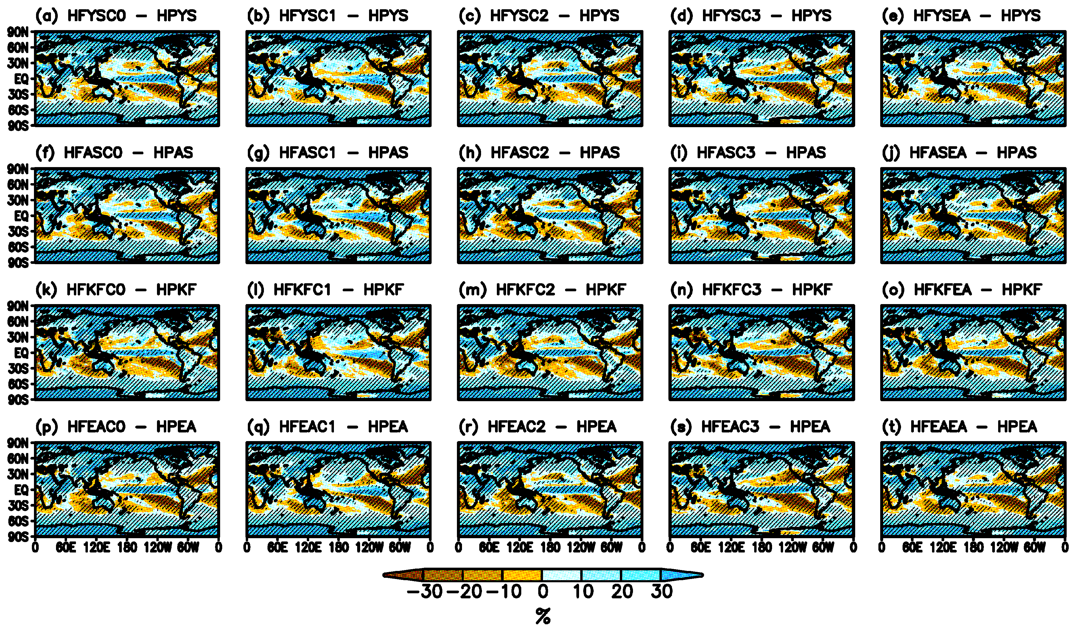
Future changes in PAV are illustrated in Figure 5. In the case of the 60-km models with YS (Figure 5a–d), the present-day simulation with the same YS of HPYS (1983–2003, 21 years) is subtracted from future simulations of HFYSC0, HFYSC1, HFYSC2 and HFYSC3 (2079–2099, 21 years) to obtain future change, which is converted into the ratio (%) to the present-day climatology HPYS. Similarly, future changes by the 60-km model with the AS and KF schemes are calculated from the present-day simulations with the corresponding same cumulus convection schemes. The statistical significance of changes is evaluated by Student’s t-test based on variances of year-to-year variability.
In the case of HFYSC0 (Figure 5a), precipitation increases over the equatorial regions of the Pacific Ocean, the Arabian Sea and the high latitudes of the Northern Hemisphere. These regions correspond to the larger warming of SST (Figure 1a). Precipitation also increases in the high latitudes of the Southern Hemisphere, but the warming of SST is relatively small in these regions (Figure 1a). This suggests that the precipitation increase in the high latitudes of the Southern Hemisphere is caused by large-scale circulation, rather than by the local SST effect. Precipitation decreases over the eastern Southern Pacific Ocean in the subtropical region around 30° S, the ocean to the west of Australia and the Atlantic Ocean in the subtropical region of the both hemispheres. These regions with decreased precipitation roughly correspond to the region with relatively small SST warming (Figure 1a). If we compare precipitation changes in Figure 5a–d, which are simulated by the same YS forced with different SSTs, the spatial structure is almost similar from the large-scale perspective, but the precipitation changes over the western tropical Pacific Ocean around Philippines differ among simulations. In the case of the 60-km models with the AS scheme (Figure 5f–i; second row) and with the KF scheme (Figure 5k–n; third row), the large-scale spatial structure is similar to those by the 60-km models with YS (Figure 5a–d; first row). However, precipitation decrease over the western tropical Pacific Ocean by the 60-km models with the KF scheme (Figure 5k–n; third row) is much more evident than the 60-km models with YS (Figure 5a–d; first row) and with the AS scheme (Figure 5f–i; second row). The dependence of precipitation change on the convection scheme is summarized by the ensemble averages (Figure 5e,j,o; last column). Precipitation increases over the western tropical Pacific Ocean by the 60-km models with YS (Figure 5e) and with the AS scheme (Figure 5j), while precipitation decreases over there by the 60-km models with the KF scheme (Figure 5o). The reason why the KF scheme behaves different from the YS and AS schemes might relate to the sensitive responses of the KF cumulus convection schemes over the MC (Figure S2), but the physical interpretation of the difference among future precipitation changes is not straightforward.
The dependence of precipitation change on SST is summarized by the ensemble averages (Figure 5p–s; bottom row). Precipitation increases over the equatorial regions of the Pacific Ocean in simulations with SST clusters C0 (Figure 5p), C2 (Figure 5r) and C3 (Figure 5s). On the other hand, in the case of C1 (Figure 5q), the region where precipitation increases over the equatorial regions of the Pacific Ocean is confined to the eastern side of the ocean and does not extend westward. This might be partly due to relatively small warming of SST in cluster C1 over the tropical Pacific Ocean compared with C0, C2 and C3 (Figure 1e–g). We will further discuss the dependence of precipitation change on convection scheme and SST in the later Section 4.3.
The ensemble average of all 12 simulations (Figure 5a–d,f–i,k–n) is displayed in Figure 5t. In general, precipitation increases globally, except some regions over the subtropical area. This suggests that global average precipitation will increase in the future. We will discuss this point from a global perspective in the later Section 4.4. The area of the statistically-significant region in the ensemble average (Figure 5t) is larger than that of individual simulations (Figure 5a–d,f–i,k–n). This is one of advantages of ensemble simulations and is mainly caused by the larger sample size (21 years/run × 12 runs = 252 years) as compared to individual simulation (21 years). The geographical distribution of precipitation change is qualitatively consistent with the Figure 12.10 in [46] based on the MME mean of CMIP5 AOGCMs.
4.2. Extreme Precipitation Events
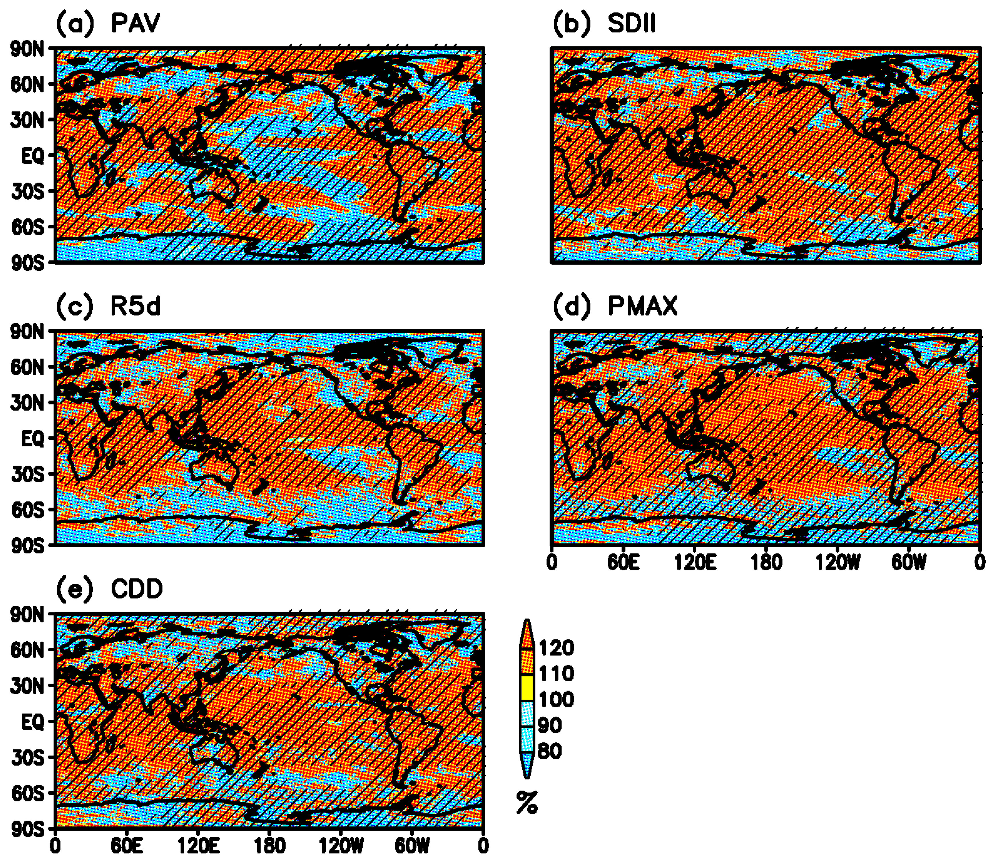
Figure 6 displays the future change in extreme precipitation events (Table 3) including PAV for comparison. Each panel is calculated from the ensemble average of all 12 simulations. The area of precipitation increase in SDII (Figure 6b) is larger than that in PAV (Figure 6a). In PAV, precipitation decreases over the Mediterranean, the southern part of Africa, the ocean to the west of Australia and in the subtropics of the South Atlantic Ocean, but in SDII, precipitation increases over these regions. Another evident difference is that precipitation decreases over the western tropical Pacific Ocean and Antarctica in SDII as opposed to the precipitation increase over these regions in PAV. In the case of R5d (Figure 6c), the distribution of change is almost similar to SDII with some differences, but the magnitude of the positive and negative change in R5d is larger than those in SDII. Unlike SDII, R5d increases over Antarctica. This inconsistency might be originating in the difference of the index definition. In the case of PMAX (Figure 6d), the distribution of change is almost similar to R5d. Unlike the precipitation indices of PAV, SDII, R5d and PMAX, the index CDD is a measure of dryness and drought possibility. Note that the color bar in CDD (Figure 6e) is reversed in contrast to the other color bars (Figure 6a–d), such that brown color means dryness. CDD increases over the Mediterranean, the subtropical regions of eastern North Pacific Ocean, the United States, the Caribbean countries, the North Atlantic Ocean and the subtropical regions in the Southern Hemisphere. Since most of these regions are dry areas in the present-day observed climate condition, the drier region will get drier in the future. Over Europe, Africa, Australia, North America and South America, both CDD (Figure 6e) and extreme precipitation events (Figure 6b–d) will increase. This suggests that rainfall events in these regions will concentrate to a short period of time, presumably leading to the increase of natural disasters, such as flood and landslide.
Our finding that the area and rate of precipitation increase for heavy rainfall (Figure 6c,d) are larger than that for mean precipitation (Figure 6a) agrees with previous studies by [47,48,49,50,51]. This is consistent with the fact that changes in the extreme precipitation follow more closely the Clausius–Clapeyron (C-C) relationship than changes in the mean precipitation [51]. We will further discuss this point in Section 4.4.
Future R5d and CDD changes over land projected by the MME mean of CMIP5 AOGCMs are illustrated in Figure 12.26 of [46]. In this figure, R5d increases almost all land area, while CDD increases over the Mediterranean, the USA, South America and the southern part of Africa. Our results are basically consistent with these changes.
4.3. Which Influences Precipitation Change, the Cumulus Convection Scheme or SST?
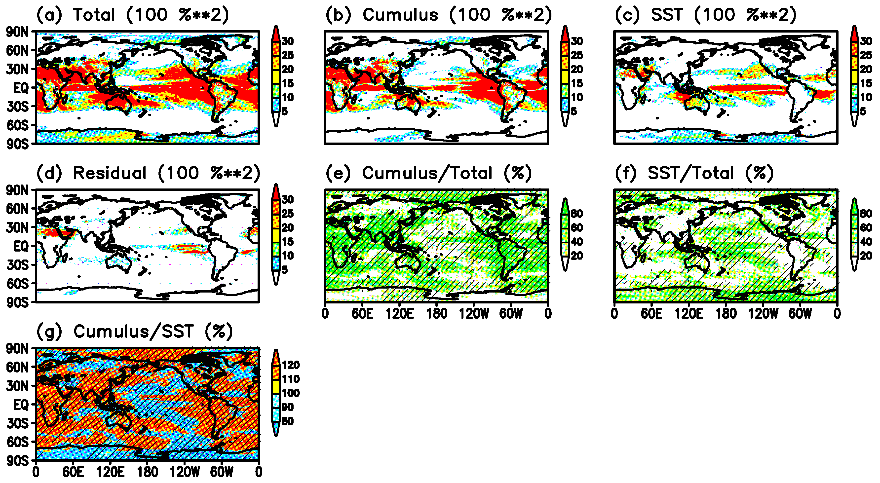
We evaluate the dependence of future precipitation change on the cumulus convection scheme and SST. For this purpose, we have applied a two-way of analysis of variance (ANOVA; [52]) to future precipitation changes by the ensemble simulations with respect to three different cumulus convection schemes and four different SST distributions (Figure 5a–d,f–i,k–n). The ANOVA is able to quantitatively separate the relative contributions of the variances originating from differences in cumulus convection schemes and from differences in SSTs to the total variance. For technical details, see the Supplemental Materials. Figure 7a displays the total variance of future precipitation changes among all 12 simulations (Figure 5a–d,f–i,k–n), which can be decomposed into contributions by cumulus convection (Figure 7b) and SST (Figure 7c). The rest of the variance is named the residual (Figure 7d), which can be interpreted as the component not explained by cumulus convection and SST or as a non-linear interaction between cumulus convection and SST. In addition, internal natural variability of the atmosphere [53] may contribute to this residual part. Normalized variances by the total variance (Figure 7a) are also shown in Figure 7e,f. Finally, the relative magnitudes of the contribution from cumulus convection and SST are illustrated in Figure 7g. In red regions, cumulus convection affects precipitation change. On the other hand, in the blue region, SST affects precipitation change. In the tropics where convection is relatively active, cumulus convection influences precipitation. As for the Pacific Ocean, SST influences precipitation on some regions in the subtropics and middle latitudes, as well as the tropics. This is partly consistent with [19] in which they stressed that the SST distribution is a dominant source of uncertainty in future precipitation change. However, as for the Atlantic Ocean, SST influences precipitation only in the northern part.
Total variance of changes in PAV is small over land at high latitudes of the Northern Hemisphere (Figure 7a). This is the outcome of the result that spatial patterns of precipitation change over these regions are almost same (Figure 5a–d,f–i,k–n), indicating that change over this region is not sensitive to the convection scheme and future SST distribution. This is caused by robust circulation changes at the 850 hPa height (Figure S8) where the spatial pattern of the height change over these regions is almost same.
We applied the ANOVA to extreme precipitation indices (Figure 8). In the case of SDII (Figure 8b), cumulus convection affects most part of the globe. As for R5d and PMAX, cumulus convection also affects most part of the globe, but SST influences some regions in the Pacific Ocean and the Atlantic Ocean. Figure 8a–c indicates that future changes in intense precipitation represented by SDII, R5D and PMAX (Figure 8b–d) are much more sensitive to the cumulus convection scheme than those by PAV (Figure 8a).
The authors in [9] have conducted similar ensemble simulations for different cumulus convections and different SSTs using the MRI-AGCM3.2S and MRI-AGCM3.2H. They used the SSTs of CMIP3 AOGCMs with the A1B scenario, whereas we used the SSTs of CMIP5 AOGCMs with RCP8.5 in this paper. They reported that the precipitation change in PAV over the tropical Pacific Ocean is much affected by SST, but that the contribution of the cumulus convection scheme to the heavy precipitation over the tropical Pacific Ocean is larger than the contribution to PAV. Our results are consistent with their results, although both results cannot be directly compared due to some differences in experimental design.
4.4. Precipitation Efficiency
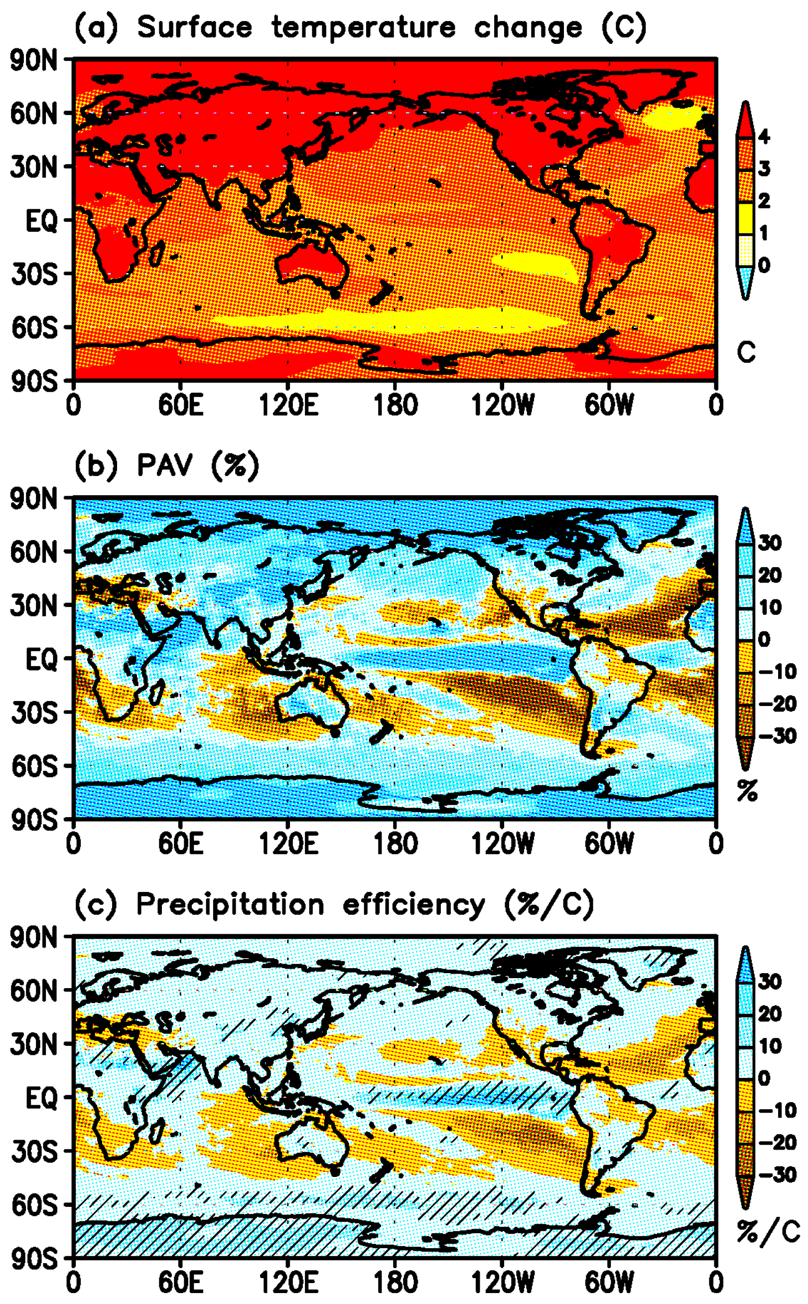
In principle, the increase in annual average precipitation and precipitation intensity can be attributed to the increased availability of water vapor caused by the warming air temperature of the atmosphere [46,54]. Figure 9a shows the future changes in annual average surface air temperature (SAT) projected by HPYS and HFYSC0. Warming over land is larger than over ocean because the heat capacity of land is smaller than that of ocean. Warming in the Northern Hemisphere is larger than in the Southern Hemisphere because the area of land in the Northern Hemisphere is larger than that in the Southern Hemisphere. Especially, warming over the high latitudes in the Norther Hemisphere is conspicuous. This is mainly caused by the surface albedo feedback mechanism. The reduction in snow over land and the extent of sea ice over the Arctic Ocean leads to the decrease of albedo at the surface, which enhances the absorption of the short wave at the surface to warm up SAT. The future change in precipitation projected by HPYS and HFYSC0 (Figure 9b) has some common features with changes in SAT (Figure 9a) in that precipitation change is generally larger over land than over ocean and is larger in the Northern Hemisphere than in the Southern Hemisphere.
Figure 9c shows the ratio of PAV change to SAT change at each grid point using the simulations of HPYS and HFYSC0. This quantity, which is the rate of precipitation change per one degree rise in SAT, can be interpreted as a kind of ‘precipitation efficiency’, which measures the conversion rate from water vapor to precipitation. This precipitation efficiency is referred to as the ‘hydrological sensitivity’ in Section 9.3.4.1 of [55]. Hereafter, we consistently use the terminology ‘precipitation efficiency’. Figure 9c shows that the distribution of precipitation efficiency basically resembles that of precipitation change (Figure 9b), but the magnitudes of precipitation efficiency over the high latitudes in the Northern Hemisphere are reduced due to the large increase of temperature there. In Figure 9c, hatched regions denote that the precipitation efficiency exceeding the value 7.5%/°C theoretically expected from the C-C relationship [21]. Precipitation efficiency is larger than the theoretical value over the equatorial region of the Pacific Ocean, the Arabian Sea and high latitudes in the Southern Hemisphere, but precipitation efficiency is smaller than the theoretical value in most parts of the globe. This implies that the dynamical effect of atmospheric circulation is reducing the local thermodynamical effect of precipitation change in most regions. Our results are consistent with the findings by [21] in which they show that the precipitation efficiency of the MME mean of CMIP3 AOGCMs exceeds the theoretical value only over the central and eastern equatorial Pacific and the western Indian Ocean. The authors in [20] have revealed that precipitation is supposed to increase slower than the C-C relationship, and the models actually match the anticipation. Our results are consistent with their findings.
We further extended our analysis to intense precipitation. Figure 10 illustrates the precipitation efficiency of R5d and PMAX, as well as PAV for comparison, using all 12 simulations. The geographical distribution of precipitation efficiency by R5d and PMAX generally resembles that by PAV. However, the area of positive regions (blue) by R5d and PMAX is larger than that by PAV, which is directly caused by the distribution of precipitation change by R5d (Figure 6c) and PMAX (Figure 6d). Another noteworthy feature is that the magnitude of positive precipitation efficiency (blue regions) by R5d and PMAX is larger than that by PAV, especially over the northern Pacific Ocean.
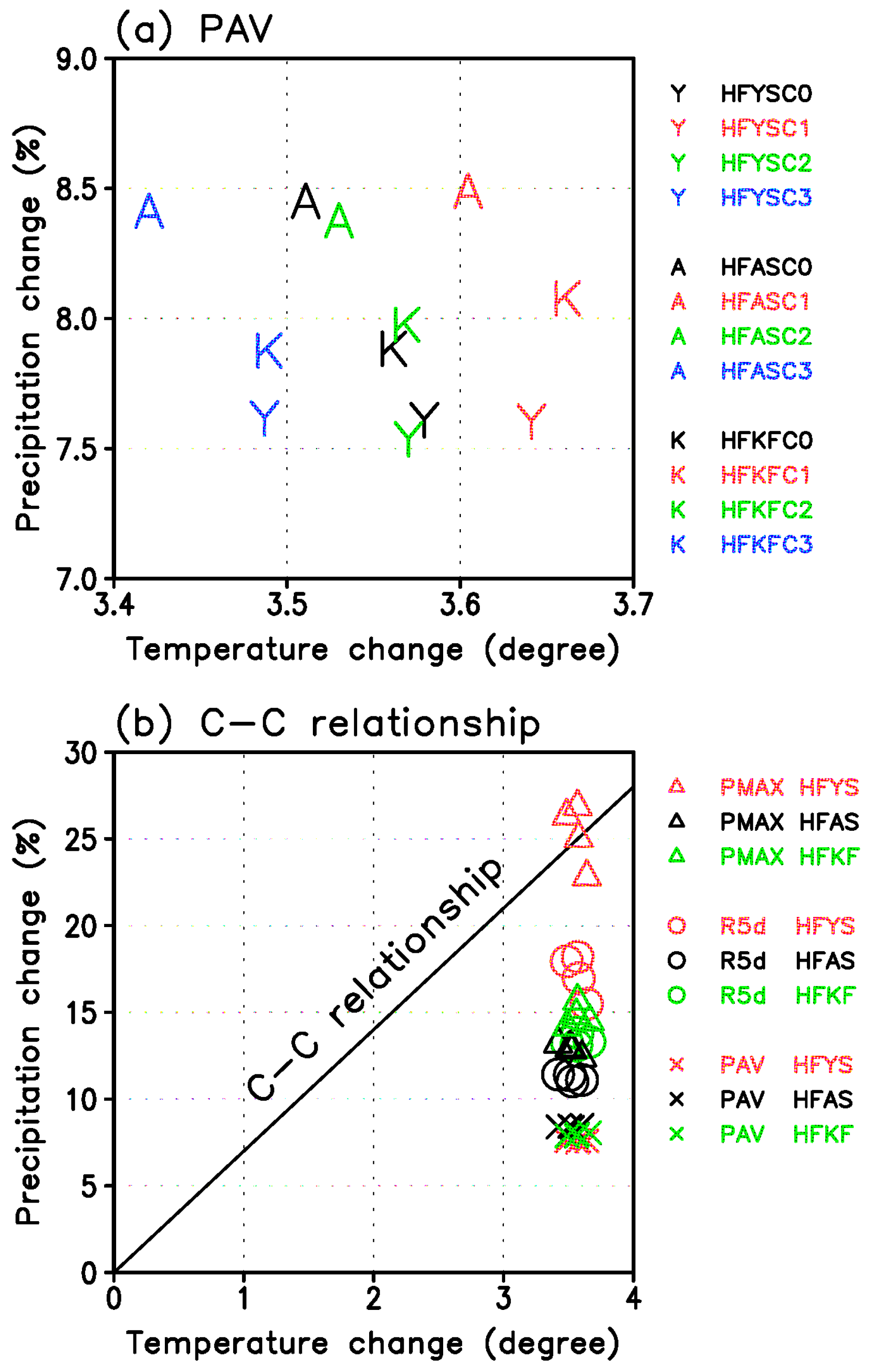
From Figure 9, we expect that the global average precipitation efficiency by R5d and PMAX might be larger than that by PAV. From a global perspective, we firstly calculated the global average of precipitation changes and SAT changes and then evaluated precipitation efficiency. This procedure smooths out the strong locality in Figure 9c and Figure 10 in which precipitation efficiency is derived at each grid point. Another intention here is to investigate the dependence of precipitation efficiency on the cumulus convection scheme and SST, because Figure 9 and Figure 10 are based on the ensemble average of all 12 simulations. Figure 11a shows the relationship between PAV changes and SAT changes for all 12 simulations. The characters denote the convection schemes, and colors denote SST clusters. Precipitation changes are mainly determined by the cumulus convection scheme (character) and are not sensitive to SST (color). For instance, precipitation changes by the AS scheme (character A) are almost the same value of about 8.4% regardless of SAT increase ranging from about 3.1–3.6 °C. Conversely, SAT changes are mainly determined by SST and are less sensitive to the cumulus convection scheme. For instance, SAT changes by SST cluster C0 (black) are almost the same value of between 3.5 and 3.6 °C, regardless of large precipitation changes. As for precipitation change, the AS scheme gives the largest changes, whereas YS gives the smallest changes. As for SAT, SST cluster C1 gives the largest warming, whereas the SST cluster C3 gives the smallest warming. HFASC3 (blue A) gives the largest precipitation efficiency 2.46%/°C = 8.40%/3.42 °C, whereas HFYSC1 (red Y) gives the smallest precipitation efficiency 2.09%/°C = 7.59%/3.64 °C. The range of precipitation efficiency of PAV is small due to the narrow range of SAT change from about 3.4–3.7 °C.
Figure 11b shows the relationship between precipitation changes and SAT changes for R5d and PMAX, as well as PAV for comparison. Note that the ranges in vertical and horizontal axes of Figure 11b are wider than those of Figure 11a. In Figure 11b, marks denote variables and colors denote the cumulus convection schemes. The differences of SST clusters are not discriminated in Figure 11b. In reference to the diagonal line indicating the theoretically-expected value of 7.5%/°C, precipitation efficiency of PAV (X mark) is far less than this value. If we focus only on the YS cumulus scheme (red), precipitation efficiency becomes larger in the following order: PAV (mark X), R5d (circle) and PMAX (triangle). The same relationship holds true for the AS scheme (black) and KF scheme (green). Since the indices PAV, R5d and PMAX represent a much more intense rainfall event in this order, Figure 11b implies precipitation changes associated with heavier rainfall events are larger than those by moderate or weak rainfall events. It is noteworthy that the precipitation efficiency of PMAX almost reaches the theoretical value of 7.5%/°C. In other words, it is reasonable that precipitation changes in heavy rainfall events are large because the conversion from water vapor into precipitation is much more effective than moderate or weak rainfall events. This is consistent with previous studies [48,49,50,51,56] in which the change of extreme precipitation is larger than that of mean precipitation.
The authors in [10] have investigated the future precipitation over East Asia using the MRI-AGCM3.2H with SSTs of CMIP3 AOGCMs assuming the A1B scenario and found that the precipitation efficiency of heavy precipitation is larger than that of mean precipitation. Our results are also consistent with their results. Using the same experiment by the study of [10], the authors in [57] have calculated precipitation efficiency over the Arctic and have revealed that precipitation efficiency of heavy precipitation is comparable or less than that of mean precipitation. This is presumably because rainfall over the Arctic is mainly caused by horizontal transport of moisture rather than cumulus convection.
5. Conclusions
In the present-day climate simulation for 1983–2003 (21 years) by the MRI-AGCM3.2H, we confirmed that the model well reproduces the global distributions of annual average precipitation and precipitation intensity. The performance of the MRI-AGCM3.2H is higher or equal to those by the CMIP5 atmospheric global models. This can be partly attributed to the higher horizontal resolution of the MRI-AGCM3.2H as compared with CMIP5 atmospheric models, because we found a statistically-significant correlation between model skill and grid size with respect to annual average precipitation and precipitation extremes.
In the future climate simulation for 2079–2099 (21 years), we have conducted the 12 ensemble simulations for three different convection schemes and four different future SST distributions, assuming the emission scenario RCP8.5. Annual average precipitation will increase over the equatorial regions and decrease over the subtropical regions. The area of precipitation increase by intense precipitation is larger than that by annual average precipitation. The differences of precipitation change among all 12 simulations are generally sensitive to the cumulus convection scheme, but changes are influenced by the SST over the some part of the Pacific Ocean. This is almost consistent with the previous work by [9], although their SST distributions are different from those used in this paper.
The precipitation efficiency defined as precipitation change per 1° surface temperature warming is evaluated. The global average of precipitation efficiency for annual precipitation was less than the maximum value expected by thermodynamical theory, indicating that dynamical atmospheric circulation is acting to reduce the conversion efficiency from water vapor to precipitation. The precipitation efficiency by intense precipitation is larger than that by moderate and weak precipitation. This agrees with previous works by [48,49,50,51,56].
Our results suggest that the selection of a convection scheme is crucial in climate simulation. Furthermore, implementing multiple cumulus convection schemes might be favorable to evaluate the spread of future precipitation change and enhance the reliability of future projection, if computer resources are rich and available. However, uncertainty in future precipitation change is often attributed to the different SST patterns among CMIP5 AOGCMs. We still recognize future projection is influenced by SST distributions, because future projected SST has also large uncertainties.
One of the major caveats in our simulations is the lack of air-sea interactions. In order to evaluate the effect of air-sea coupling process, we have already finished the future climate projection using the MRI-AGCM3.2H coupled with a full ocean model [18]. Figure S9 shows the difference between future precipitation changes projected by an atmospheric model and a coupled model. As is expected, differences are large over the eastern tropical Pacific Ocean. The reason and mechanism of the difference is not yet fully analyzed and should be explored in future studies.
Supplementary Materials
The following are available online at www.mdpi.com/2073-4433/8/5/91/s1: Table S1: Previous studies on precipitation using the MRI-AGCM3, Table S2: Features of 24 CMIP5 models used in this study, Figure S1: Comparison among observations for PAV, Figure S2: Comparison among simulations for PAV, Figure S3: Same as Figure S2 but for R5d, Figure S4: Root mean square errors of global distribution of precipitation indices between observations by GPCP 1ddv1.2 and model simulations, Figure S5: Same as Figure S4 but for bias, Figure S6: Dependence of model skill on the grid spacing of 31 models including 7 MRI-AGCM3.2 models and 24 CMIP5 atmospheric models, Figure S7: Correlation coefficients between the skill and grid size of 31 models, Figure S8: Same as Figure 5 but for 850 hPa height, Figure S9: Comparison between future changes in PAV by atmospheric model and AOGCM, ANalysis Of VAriance (ANOVA): Technical details.
Acknowledgments
This work was conducted under the framework of “the Integrated Research Program for Advanced Climate Modeling” supported by the TOUGOU Program of the Ministry of Education, Culture, Sports, Science, and Technology (MEXT) of Japan. We also thank the anonymous reviewers whose valuable comments and suggestions greatly improved the manuscript.
Conflicts of Interest
The authors declare no conflict of interest.
References
- Cubasch, U.; Wuebbles, D.; Chen, D.; Facchini, M.C.; Frame, D.; Mahowald, N.; Winther, J.-G. Introduction. In Climate Change 2013: The Physical Science Basis; Contribution of Working Group I to the Fifth Assessment Report of the Intergovernmental Panel on Climate Change; Stocker, T.F., Qin, D., Plattner, G.-K., Tignor, M., Allen, S.K., Boschung, J., Nauels, A., Xia, Y., Bex, V., Midgley, P.M., Eds.; Cambridge University Press: Cambridge, UK; New York, NY, USA, 2013. [Google Scholar]
- Shiogama, H.; Watanabe, M.; Ogura, T.; Yokohata, T.; Kimoto, M. Multi-parameter multi-physics ensemble (MPMPE): A new approach exploring the uncertainties of climate sensitivity. Atmos. Sci. Lett. 2014, 15, 97–102. [Google Scholar] [CrossRef]
- Kusunoki, S.; Yoshimura, J.; Yoshimura, H.; Noda, A.; Oouchi, K.; Mizuta, R. Change of Baiu rain band in global warming projection by an atmospheric general circulation model with a 20-km grid size. J. Meteorol. Soc. Jpn. 2006, 84, 581–611. [Google Scholar] [CrossRef]
- Kitoh, A.; Kusunoki, S. East Asian summer monsoon simulation by a 20-km mesh AGCM. Clim. Dyn. 2007, 31, 389–401. [Google Scholar] [CrossRef]
- Kusunoki, S. Is the global atmospheric model MRI-AGCM3.2 better than the CMIP5 atmospheric models in simulating precipitation over East Asia? Clim. Dyn. 2016, 1–22. [Google Scholar] [CrossRef]
- Kusunoki, S.; Mizuta, R. Future Changes in the Baiu Rain Band Projected by a 20-km Mesh Global Atmospheric Model: Sea Surface Temperature Dependence. Sci. Online Lett. Atmos. 2008, 4, 85–88. [Google Scholar] [CrossRef]
- Kusunoki, S.; Mizuta, R.; Matsueda, M. Future changes in the East Asian rain band projected by global atmospheric models with 20-km and 60-km grid size. Clim. Dyn. 2011, 37, 2481–2493. [Google Scholar] [CrossRef]
- Kusunoki, S.; Mizuta, R. Comparison of near future (2015–2039) changes in the East Asian rain band with future (2075–2099) changes projected by global atmospheric models with 20-km and 60-km grid size. Sci. Online Lett. Atmos. 2012, 8, 73–76. [Google Scholar] [CrossRef]
- Endo, H.; Kitoh, A.; Ose, T.; Mizuta, R.; Kusunoki, S. Future changes and uncertainties in Asian precipitation simulated by multiphysics and multi-sea surface temperature ensemble experiments with high-resolution Meteorological Research Institute atmospheric general circulation models (MRI-AGCMs). J. Geophys. Res. 2012, 117, D16118. [Google Scholar] [CrossRef]
- Kusunoki, S.; Mizuta, R. Changes in precipitation intensity over East Asia during the 20th and 21st centuries simulated by a global atmospheric model with a 60 km grid size. J. Geophys. Res. Atmos. 2013, 118, 11007–11016. [Google Scholar] [CrossRef]
- Kitoh, A.; Endo, H. Changes in precipitation extremes projected by a 20-km mesh global atmospheric model. Weather Clim. Extremes 2016, 11, 41–52. [Google Scholar] [CrossRef]
- Mizuta, R.; Murata, A.; Ishii, M.; Shiogama, H.; Hibino, K.; Mori, N.; Arakawa, O.; Imada, Y.; Yoshida, K.; Aoyagi, T.; et al. Over 5000 years of ensemble future climate simulations by 60 km global and 20 km regional atmospheric models. Bull. Am. Meteorol. Soc. 2016. [Google Scholar] [CrossRef]
- Endo, H.; Kitoh, A.; Mizuta, R.; Ishii, M. Future changes in precipitation extremes in East Asia and their uncertainty based on large ensemble simulations with a high resolution AGCM. Sci. Online Lett. Atmos. 2017, 13, 7–12. [Google Scholar] [CrossRef]
- Kusunoki, S. Future changes in precipitation over East Asia projected by the global atmospheric model MRI-AGCM3.2. Clim. Dyn. 2017, 1–17. [Google Scholar] [CrossRef]
- Bengtsson, L.; Hodges, K.I.; Keenlyside, N. Will extratropical storms intensify in a warmer climate? J. Clim. 2009, 22, 2276–2301. [Google Scholar] [CrossRef]
- Douville, H. Impact of regional SST anomalies on the Indian Monsoon response to global waming in the CNRM climate model. J. Clim. 2005, 19, 2008–2024. [Google Scholar] [CrossRef]
- Hasegawa, A.; Emori, S. Effect of air-sea coupling in the assessment of CO2-induced intensification of tropical cyclone activity. Geophys. Res. Lett. 2007, 34, L05701. [Google Scholar] [CrossRef]
- Ogata, T.; Mizuta, R.; Adachi, Y.; Murakami, H.; Ose, T. Effect of air-sea coupling on the frequency distribution of intense tropical cyclones over the northwestern Pacific. Geophys. Res. Lett. 2015, 42, 10415–10421. [Google Scholar] [CrossRef]
- Ma, J.; Xie, S.-P. Regional Patterns of Sea Surface Temperature Change: A Source of Uncertainty in Future Projections of Precipitation and Atmospheric Circulation. J. Clim. 2013, 26, 2482–2501. [Google Scholar] [CrossRef]
- Held, I.M.; Soden, B.J. Robust Responses of the Hydrological Cycle to Global Warming. J. Clim. 2006, 19, 5686–5699. [Google Scholar] [CrossRef]
- Vecchi, G.A.; Soden, B.J. Global warming and the weakening of the tropical circulation. J. Clim. 2007, 20, 4316–4340. [Google Scholar] [CrossRef]
- Mizuta, R.; Yoshimura, H.; Murakami, H.; Matsueda, M.; Endo, H.; Ose, T.; Kamiguchi, K.; Hosaka, M.; Sugi, M.; Yukimoto, S.; et al. Climate simulations using MRI-AGCM3.2 with 20-km grid. J. Meteorol. Soc. Jpn. 2012, 90A, 233–258. [Google Scholar] [CrossRef]
- Yoshimura, H.; Mizuta, R.; Murakami, H. A spectral cumulus parameterization scheme interpolating between two convective updrafts with semi-lagrangian calculation of transport by compensatory subsidence. Mon. Weather Rev. 2015, 143, 597–621. [Google Scholar] [CrossRef]
- Tiedtke, M. A comprehensive mass flux scheme for cumulus parameterization in large-scale models. Mon. Weather Rev. 1989, 117, 1779–1800. [Google Scholar] [CrossRef]
- Randall, D.A.; Pan, D.M. Implementation of the Arakawa-Schubert cumulus parameterization with a prognostic closure. In The Representation of Cumulus Convection in Numerical Models; American Meteorological Society: Boston, MA, USA, 1993; Volume 24, Chapter 11, No. 46; pp. 137–147. [Google Scholar]
- Kain, J.S.; Fritsch, J.M. A one-dimensional entraining/detraining plume model and its application in convective parameterization. J. Atmos. Sci. 1990, 47, 2784–2802. [Google Scholar] [CrossRef]
- Yukimoto, S.; Yoshimura, H.; Hosaka, M.; Sakami, T.; Tsujino, H.; Hirabara, M.; Tanaka, T.; Deushi, M.; Obata, A.; Nakano, H.; et al. Meteorological Research Institute—Earth System Model Version 1 (MRI-ESM1)—Model Description; Technical Reports of the Meteorological Research Institute; Meteorological Research Institute: Tsukuba, Japan, 2011; Volume 64, p. 88. [Google Scholar]
- Rayner, N.A.; Parker, D.E.; Horton, E.B.; Folland, C.K.; Alexander, L.V.; Rowell, D.P.; Kent, E.C.; Kaplan, A. Global analyses of sea surface temperature, sea ice, and night marine air temperature since the late nineteenth century. J. Geophys. Res. 2003, 108, 4407–4437. [Google Scholar] [CrossRef]
- Collins, M.; Knutti, R.; Arblaster, J.; Dufresne, J.-L.; Fichefet, T.; Friedlingstein, P.; Gao, X.; Gutowski, W.J.; Johns, T.; Krinner, G.; et al. Section 12; Long-term Climate Change: Projections, Commitments and Irreversibility. In Climate Change 2013: The Physical Science Basis; Contribution of Working Group I to the Fifth Assessment Report of the Intergovernmental Panel on Climate Change; Stocker, T.F., Qin, D., Plattner, G.-K., Tignor, M., Allen, S.K., Boschung, J., Nauels, A., Xia, Y., Bex, V., Midgley, P.M., Eds.; Cambridge University Press: Cambridge, UK; New York, NY, USA, 2013. [Google Scholar]
- Mizuta, R.; Adachi, Y.; Yukimoto, S.; Kusunoki, S. Estimation of the Future Distribution of Sea Surface Temperature and Sea Ice Using the CMIP3 Multi-Model Ensemble Mean; Technical Reports of the Meteorological Research Institute; Meteorological Research Institute: Tsukuba, Japan, 2008; Volume 56, p. 28. [Google Scholar]
- Mizuta, R.; Arakawa, O.; Ose, T.; Kusunoki, S.; Endo, H.; Kitoh, A. Classification of CMIP5 future climate responses by the tropical sea surface temperature changes. SOLA 2014, 10, 167–171. [Google Scholar] [CrossRef]
- Intergovermental Panel on Climate Change (IPCC). Special Report on Emissions Scenarios: A Special Report of Working Group III of the Intergovernmental Panel on Climate Change; Nakicenovic, N., Alcamo, J., Davis, G., de Vries, B., Fenhann, J., Gaffin, S., Gregory, K., Grübler, A., Jung, T.Y., Kram, T., et al., Eds.; Cambridge University Press: Cambridge, UK, 2000; p. 599. [Google Scholar]
- Shibata, K.; Deushi, M.; Sekiyama, T.T.; Yoshimura, H. Development of an MRI chemical transport model for the study of stratospheric chemistry. Pap. Meteorol. Geophys. 2004, 55, 75–119. [Google Scholar] [CrossRef]
- Huffman, G.J.; Adler, R.F.; Morrissey, M.M.; Bolvin, D.T.; Curtis, S.; Joyce, R.; McGavock, B.; Susskind, J. Global precipitation at one-degree daily resolution from multisatellite observations. J. Hydrometeorol. 2001, 2, 36–50. [Google Scholar] [CrossRef]
- Sperber, K.R.; Annamalai, H.; Kang, I.S.; Kitoh, A.; Moise, A.; Turner, A.G.; Wang, B.; Zhou, T. The Asian summer monsoon: An intercomparison of CMIP5 vs. CMIP3 simulations of the late 20th century. Clim. Dyn. 2013, 41, 2711–2744. [Google Scholar] [CrossRef]
- Adler, R.F.; Huffman, G.J.; Chang, A.; Ferrano, R.; Xie, P.P.; Janowiak, J.; Rudolf, B.; Schneider, U.; Curtis, S.; Bolvin, D.; et al. The Version-2 Global Precipitation Climatology Preject (GPCP) monthly precipitation analysis (1979–Present). J. Hydrometeorol. 2003, 4, 1147–1167. [Google Scholar] [CrossRef]
- Xie, P.; Arkin, P. Global precipitation: A 17-year monthly analysis based on gauge observations, satellite estimates and numerical model outputs. Bull. Am. Meteorol. Soc. 1997, 78, 2539–2558. [Google Scholar] [CrossRef]
- Huffman, G.J.; Adler, R.F.; Bolvin, D.T.; Gu, G.; Nelkin, E.J.; Bowman, K.P.; Hong, Y.; Stocker, E.F.; Wolff, D.B. The TRMM Multisatellite Precipitation Analysis (TMPA): Quasi-global, multiyear, combined-sensor precipitation estimates at fine scales. J. Hydrometeorol. 2007, 8, 38–55. [Google Scholar] [CrossRef]
- Minobe, S.; Kuwano-Yoshida, A.; Komori, N.; Xie, S.-P.; Small, R.J. Influence of the Gulf Stream on the troposphere. Nature 2008, 452, 206–209. [Google Scholar] [CrossRef] [PubMed]
- Taylor, K.E. Summarizing multiple aspects of model performance in a single diagram. J. Geophys. Res. 2001, 106, 7183–7192. [Google Scholar] [CrossRef]
- Lambert, S.J.; Boer, G.J. CMIP1 evaluation and intercomparison of coupled climate models. Clim. Dyn. 2001, 17, 83–106. [Google Scholar] [CrossRef]
- Gleckler, P.J.; Taylor, K.E.; Doutriaux, C. Performance metrics for climate models. J. Geophys. Res. 2008, 113, D06104. [Google Scholar] [CrossRef]
- Reichler, T.; Kim, J. How well do coupled models simulate today’s climate? Bull. Am. Meteorol. Soc. 2008, 89, 303–311. [Google Scholar] [CrossRef]
- Frich, P.; Alexander, L.V.; Della-Marta, P.; Gleason, B.; Haylock, M.; Klein Tank, A.M.G.; Peterson, T. Observed coherent changes in climatic extremes during the second half of the twentieth century. Clim. Res. 2002, 19, 193–212. [Google Scholar] [CrossRef]
- Dai, A. Precipitation characteristics in eighteen coupled climate models. J. Clim. 2006, 19, 4605–4630. [Google Scholar] [CrossRef]
- Intergovernmental Panel on Climate Change (IPCC). Climate Change 2013: The Physical Science Basis; Contribution of Working Group I to the Fifth Assessment Report of the Intergovernmental Panel on Climate Change; Stocker, T.F., Qin, D., Plattner, G.K., Tignor, M., Allen, S.K., Boschung, J., Nauels, A., Xia, Y., Bex, V., Midgley, P.M., Eds.; Cambridge University Press: Cambridge, UK; New York, NY, USA, 2013; p. 1535. [Google Scholar]
- Hennessy, K.J.; Gregory, J.M.; Mitchell, J.F.B. Changes in daily precipitation under enhanced greenhouse conditions. Clim. Dyn. 1997, 13, 667–680. [Google Scholar] [CrossRef]
- Kharin, V.V.; Zwiers, F.W. Changes in the extremes in an ensemble of transient climate simulations with a coupled atmosphere-ocean GCM. J. Clim. 2000, 13, 3760–3788. [Google Scholar] [CrossRef]
- Wehner, M.F. Predicted 21st century changes in seasonal extreme precipitation events in the Parallel Climate Model. J. Clim. 2004, 17, 4281–4290. [Google Scholar] [CrossRef]
- Emori, S.; Brown, S.J. Dynamic and thermodynamic changes in mean and extreme precipitation under changed climate. Geophys. Res. Lett. 2005, 32, L17706. [Google Scholar] [CrossRef]
- Pall, P.; Allen, M.R.; Stone, D.A. Testing the Clausius-Clapeyron constraint on changes in extreme precipitation under CO2 warming. Clim. Dyn. 2007, 28, 351–363. [Google Scholar] [CrossRef]
- Storch, H.V.; Zwiers, F.W. Section 9 Analysis of Variance. In Statistical Analysis in Climate Research; Storch, H.V., Zwiers, F.W., Eds.; Cambridge University Press: Cambridge, UK, 1999; pp. 171–192. [Google Scholar]
- Deser, C.; Knutti, R.; Solomon, S.; Phillips, A.S. Communication of the role of natural variability in future North American climate. Nat. Clim. Chang. 2012, 2, 775–779. [Google Scholar] [CrossRef]
- Intergovernmental Panel on Climate Change (IPCC). Climate Change 2007: The Physical Science Basis; Contribution of Working Group I to the Fourth Assessment Report of the Intergovernmental Panel on Climate Change; Solomon, S., Qin, D., Manning, M., Chen, Z., Marquis, M., Averyt, K.B., Tignor, M., Miller, H.L., Eds.; Cambridge University Press: Cambridge, UK; New York, NY, USA, 2007; p. 996. [Google Scholar]
- Intergovernmental Panel on Climate Change (IPCC). Climate Change 2001: The Scientific Basis; Contribution of Working Group I to the Third Assessment Report of the Intergovernmental Panel on Climate Change; Houghton, J.T., Ding, Y., Griggs, D.J., Noguer, M., van der Linden, P.J., Dai, X., Maskell, K., Johnson, C.A., Eds.; Cambridge University Press: Cambridge, UK; New York, NY, USA, 2001; p. 881. [Google Scholar]
- Hegerl, G.C.; Zwiers, F.W.; Stott, P.A.; Kharin, V.V. Detectability of anthropogenic changes in annual temperature and precipitation extremes. J. Clim. 2004, 17, 3683–3700. [Google Scholar] [CrossRef]
- Kusunoki, S.; Mizuta, R.; Hosaka, M. Future changes in precipitation intensity over the Arctic projected by a global atmospheric model with a 60-km grid size. Polar Sci. 2015, 9, 277–292. [Google Scholar] [CrossRef]
Figure 1.
Annual mean sea surface temperature (SST) change (K) from the present-day (1979–2003, historical simulation) and the future (2075–2099, RCP8.5 scenario). (a) The composite of a total 28 models (C0); (b) the composite of the cluster C1; (c) C2; (d) C3; (e–g) differences for each cluster from the total mean (C0). The regions where over 75% of the models agree with the sign of the difference are colored. Contours denote zero. The change is normalized by the tropical (30° S–30° N) mean for each model before making the composition and then multiplied by the 28 models’ mean tropical SST change (2.74 K). From [31].
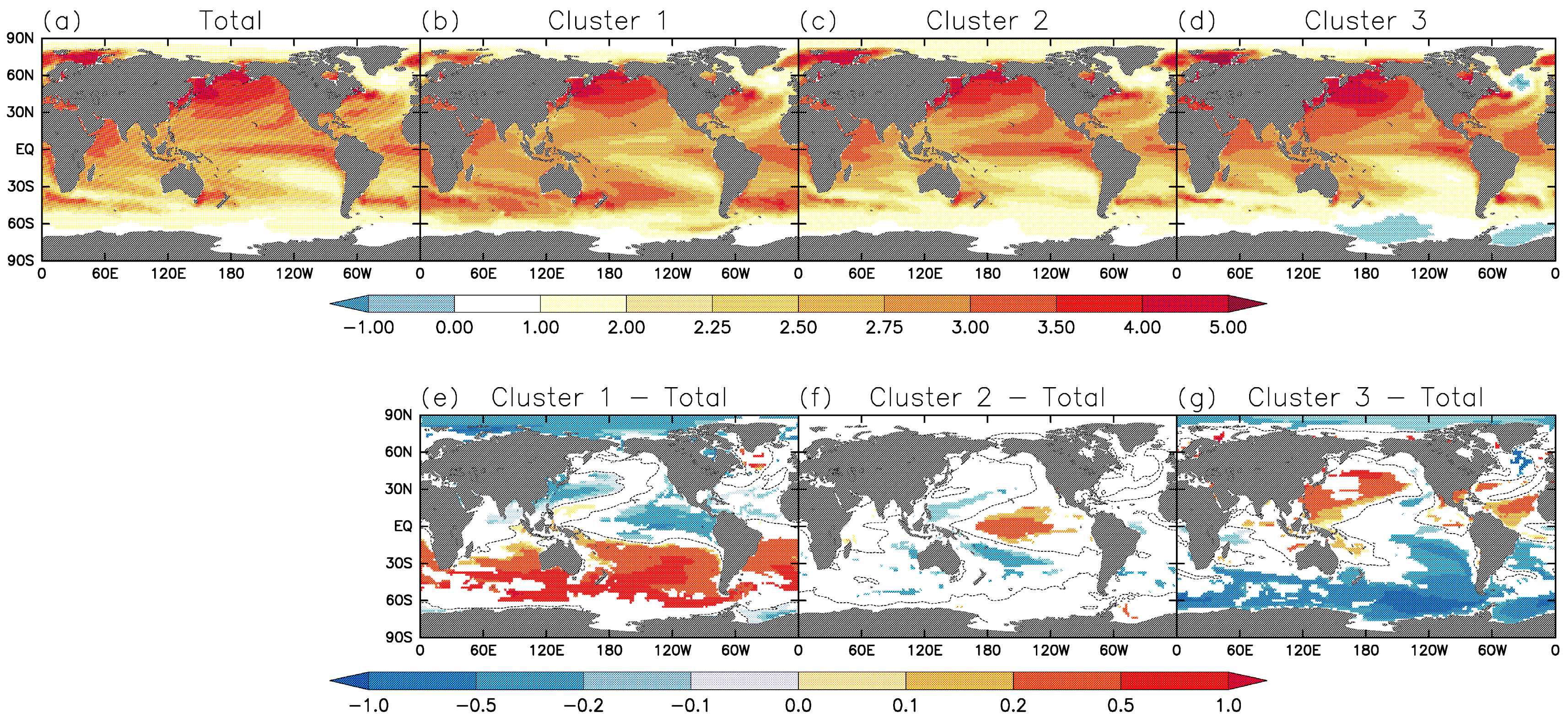
Figure 2.
The climatology of annual average precipitation (PAV). Unit is mm day−1. (a–d) Observation (Table 2); (e–h) simulations by models averaged for 1983–2003 (21 years); (e) HPYS; (f) HPAS; (g) HPKF; (h) MME mean of 24 CMIP5 atmospheric models’ Atmospheric Model Intercomparison Project (AMIP) runs (Table S1); (i–l) bias against GPCP 1ddv1.2 (a). GPCP, Global Precipitation Climatology Project.
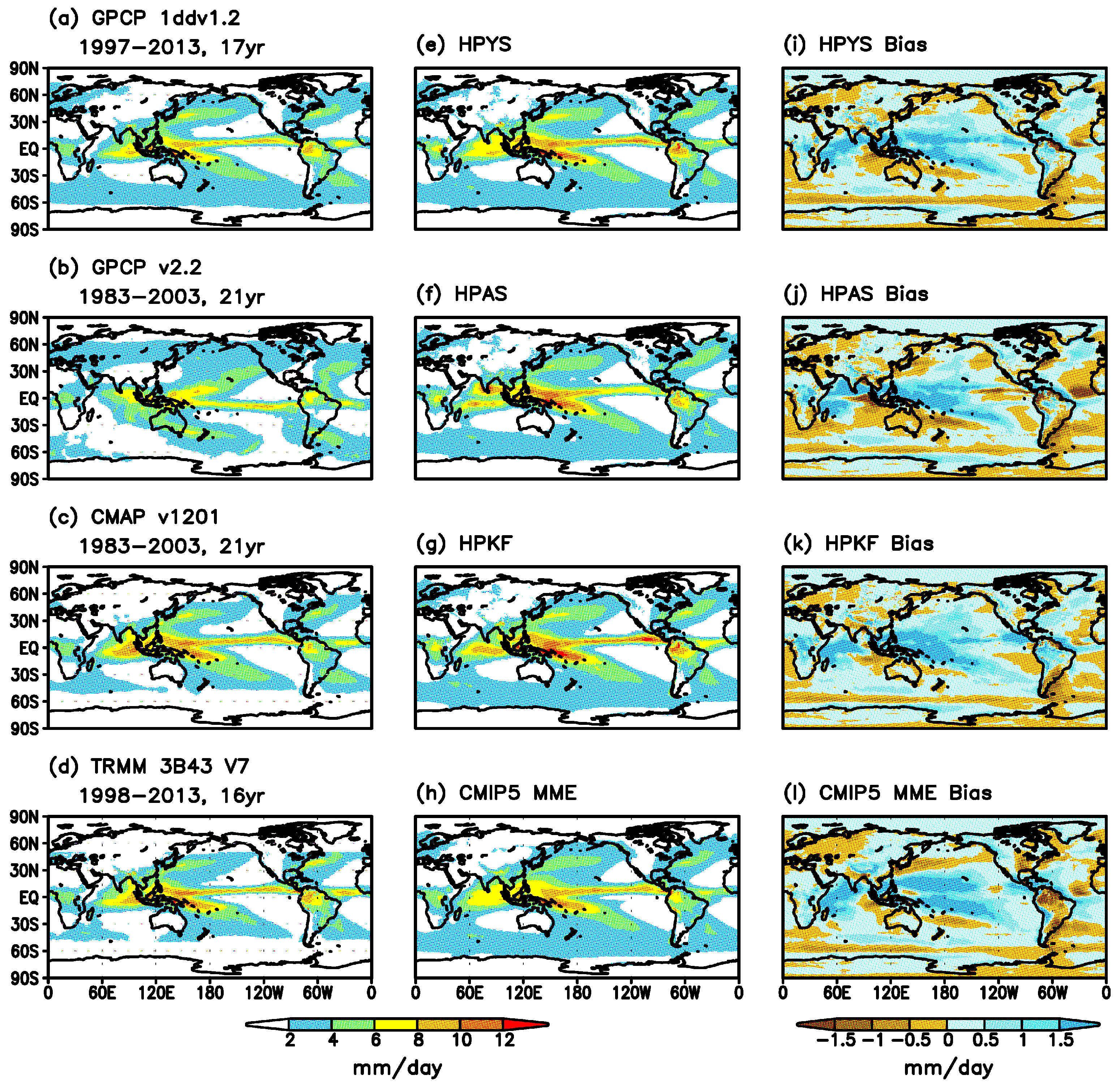
Figure 3.
Skill of PAV simulated by models verified against the GPCP 1dd V1.2 data (green circle) for the global domain. Green marks denote other observations (Table 2). Color characters show the MRI-AGCM3.2H models. Red, orange and blue characters denote the YS, AS and KF schemes, respectively. Black marks X show the CMIP5 individual models. Black circles indicate the MME mean. Black squares indicate the average of the skill scores of all of the CMIP5 models (AVM). The target domain is the same as in Figure 2. (a) The root mean square error (RMSE) and bias (mm day−1). The domain average of observation is shown above the panel. (b) Taylor diagram for displaying pattern statistics [40]. The standard deviation of the observation in the domain is shown above the panel. The contour shows the value of Taylor skill S.

Figure 4.
Spatial correlation coefficients of the global distribution of precipitation indices (Table 3) between observations by GPCP 1ddv1.2 and model simulations. Red, orange and blue bars denote the 60-km models with the YS, AS and KF schemes, respectively. Black bars show the CMIP5 individual models. Green circles indicate the MME mean of CMIP5 models. Green bars indicate the AVM of CMIP5 models. CDD, consecutive dry days.
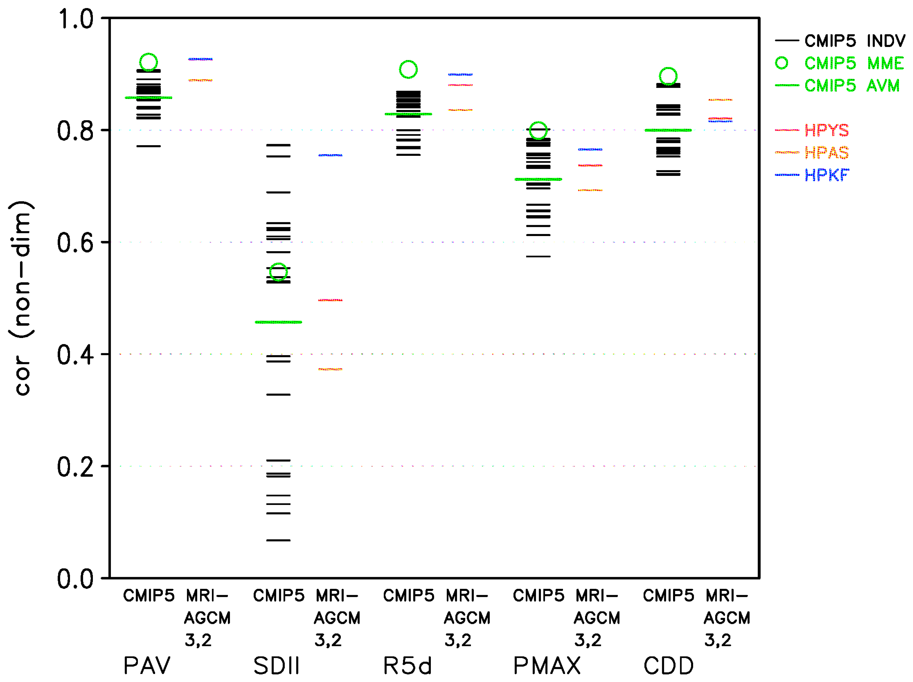
Figure 5.
Future changes (2079–2099) in annual average precipitation (%) from the present-day climatology (1983–2003). Change is normalized by the present-day climatology. Hatched regions show changes above the 95% significance level based on Student’s t-test. (First row; (a–e)) The 60-km model with YS. Changes are calculated from the present-day climate simulations with YS. (Second row; (f–i)) The 60-km model with the AS scheme. Changes are calculated from the present-day climate simulations with the AS scheme. (Third row; (k–o)) The 60-km model with the KF scheme. Changes are calculated from the present-day climate simulations with the KF scheme. (Fourth row; (p–t)) The ensemble average of 60-km model with the three convection schemes (first–third row). (First column; (a,f,k,p)) Simulations with the SST cluster C0. (Second column) Simulations with C1. (Third column) Simulations with C2. (Fourth column) Simulations with C3. (Fifth column) The ensemble average of simulations with the four SSTs (first–fourth column).

Figure 6.
Future changes in precipitation indices (Table 3) by averaging all 12 simulations. Change is normalized by the present-day climatology. Unit is %. Hatched regions show changes above the 95% significance level. (a) PAV; (b) SDII; (c) R5d; (d) PMAX; (e) CDD. (a) is the same as Figure 5t.
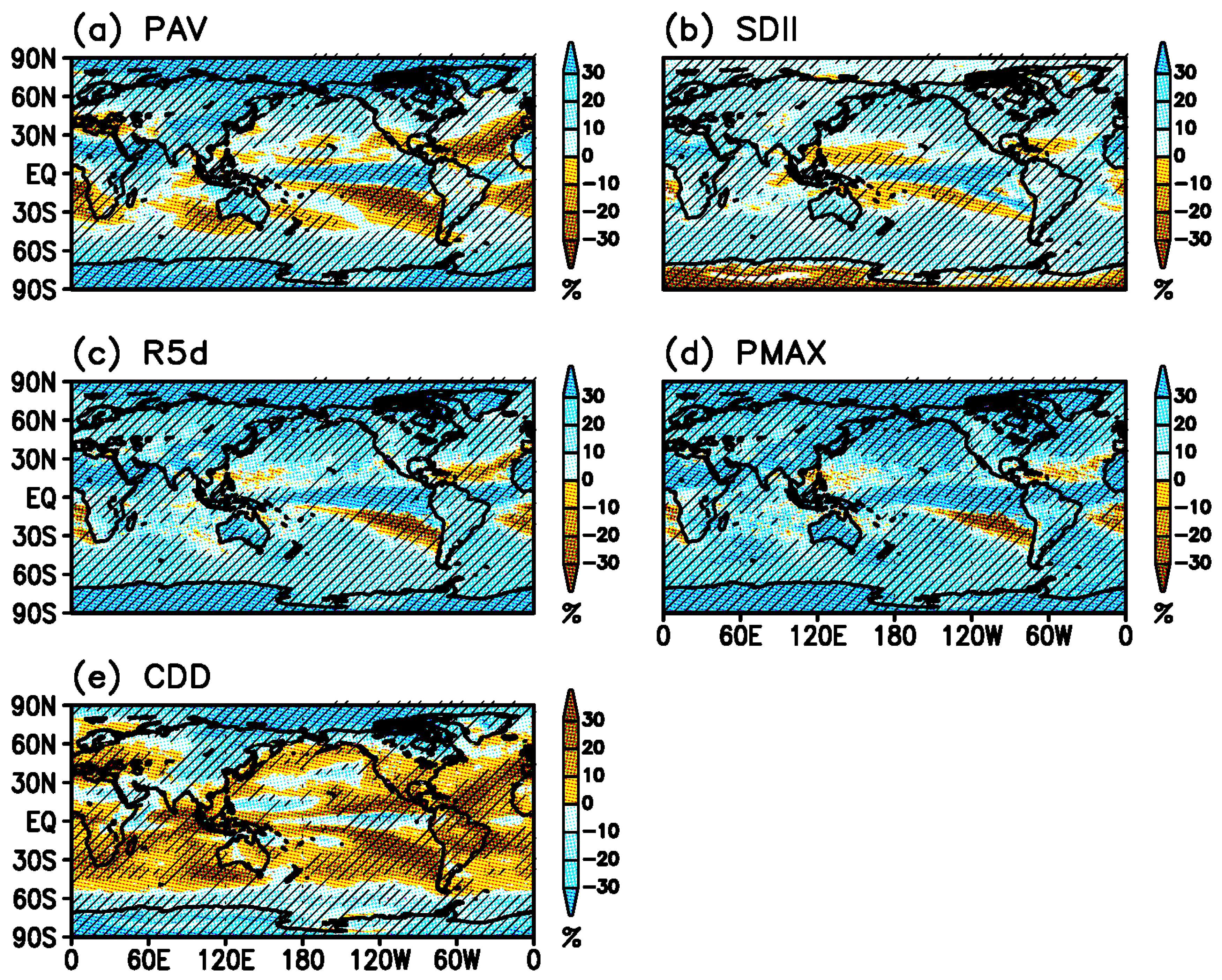
Figure 7.
A two-way analysis of variance (ANOVA; [52]) applied to future annual average precipitation changes by all 12 ensemble simulations with respect to three different cumulus convection schemes and four different SST distributions (Figure 6a–d,f–i,k–n). (a) Total variance (100%2); (b) variance due to convection scheme (100%2); (c) variance due to SST (100%2); (d) residual of variance (100%2); (e) relative contribution of cumulus convection scheme as the ratio to the total variance (%); (f) relative contribution of SST as the ratio to the total variance (%); (g) ratio (%) of the variance by the cumulus convection scheme (b) to the variance by SST (c). Hatches show regions above the 95% significance level based on the F-test.

Figure 8.
Ratio (%) of the variance by the cumulus convection scheme to the variance by SST. The ANOVA is applied for future changes in precipitation indices (Table 3). Hatched regions show the ratio above the 95% significance level. (a) PAV; (b) SDII; (c) R5d; (d) PMAX; (e) CDD. (a) is the same as Figure 7g.

Figure 9.
Precipitation efficiency calculated at each grid point. (a) Change in annual mean surface air temperature (°C) by HFYSC0 (2079–2099) from the HPYS (1983–2003); (b) PAV change (%) by HFYSC0 relative to HPYS; (c) precipitation efficiency (%/°C) defined as PAV change (b) divided by surface air temperature change (a). Hatched regions indicate that precipitation efficiency is larger than the rate of precipitation increase (7.5%/°C) expected from the Clausius–Clapeyron (C-C) relationship.

Figure 10.
The averages of the precipitation efficiency (%/°C) of all 12 simulations. (a) PAV; (b) R5d; (c) PMAX. Hatched regions indicate that precipitation efficiency is larger than the rate of precipitation increase (7.5%/°C) expected from the C-C relationship.
Figure 10.
The averages of the precipitation efficiency (%/°C) of all 12 simulations. (a) PAV; (b) R5d; (c) PMAX. Hatched regions indicate that precipitation efficiency is larger than the rate of precipitation increase (7.5%/°C) expected from the C-C relationship.
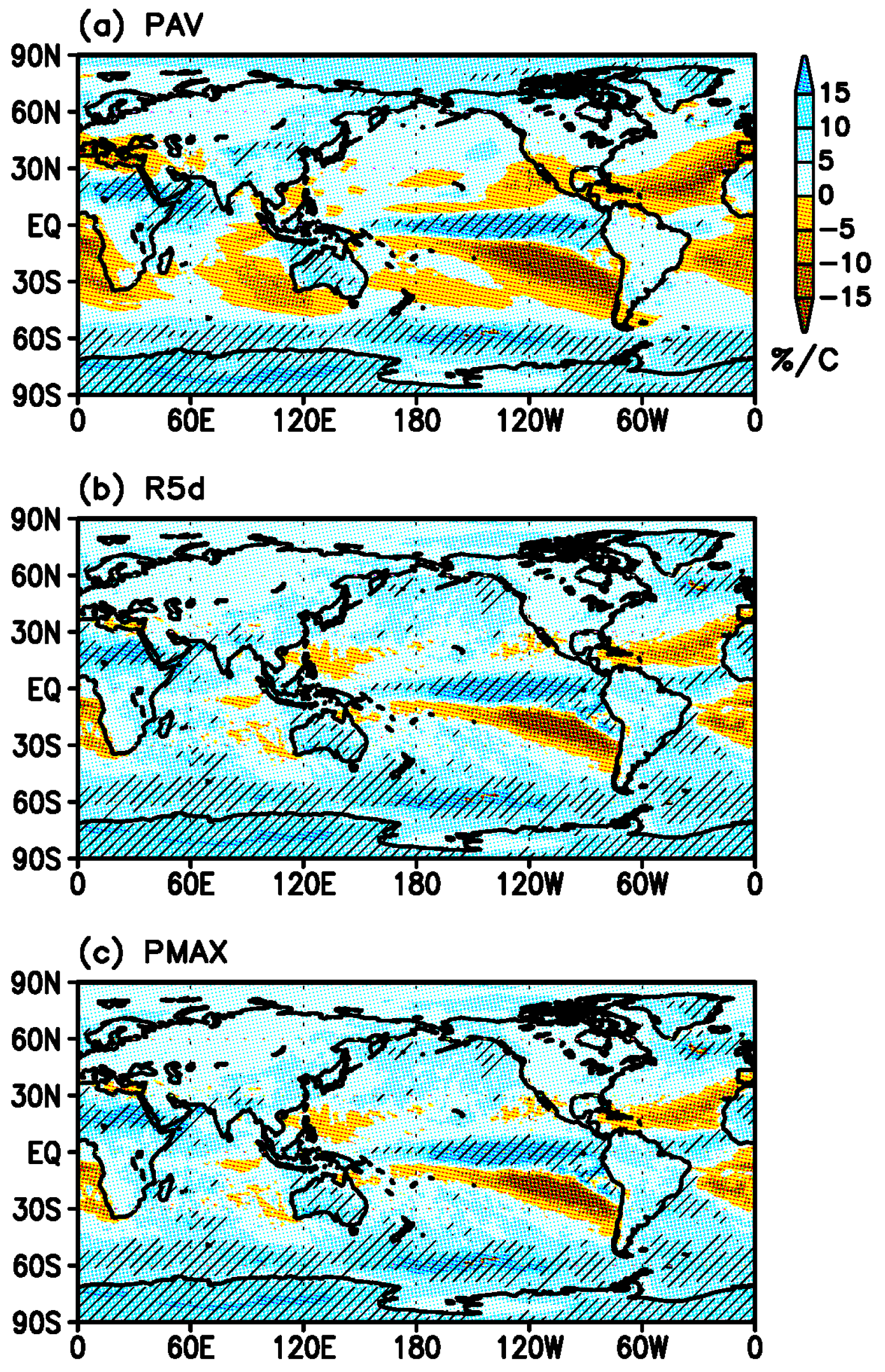
Figure 11.
Dependence of precipitation change (%) on global average annual mean surface temperature change (°C). (a) Dependence of PAV changes on the cumulus convection scheme and SST. Characters Y, A and K mean the YS, AS and KF schemes, respectively. Black, red, green and blue colors mean SST cluster C0, C1, C2 and C3, respectively. (b) Dependence of precipitation change on different indices. The black slanted line denotes the rate of precipitation increase (7.5%/°C) expected from the Clausius–Clapeyron relationship. The X mark, circle and triangle mean PAV, R5d and PMAX, respectively. Red, black and green colors mean the YS, AS and KF schemes, respectively.


Table 1.
Definition of simulation names.
| Present-Day Climate: 1983–2003, 21 Years | ||||
|---|---|---|---|---|
| Cumulus Convection a | Sea Surface Temperature (SST): Observation by the HadISST1 [28] | |||
| YS | HPYS | |||
| AS | HPAS | |||
| KF | HPKF | |||
| Future Climate: 2079–2099, 21 years | ||||
| Cumulus Convection a | Sea surface Temperature (SST): Projections by the CMIP5 AOGCMs for the Emission Scenario RCP8.5 | |||
| Cluster 0 MME | Cluster 1 | Cluster 2 | Cluster 3 | |
| YS | HFYSC0 | HFYSC1 | HFYSC2 | HFYSC3 |
| AS | HFASC0 | HFASC1 | HFASC2 | HFASC3 |
| KF | HFKFC0 | HFKFC1 | HFKFC2 | HFKFC3 |
First character of simulation name denotes horizontal resolution: H = 60 km; Second character denotes the target period: P = present-day, F = Future; Third and fourth characters denote the type of cumulus convection scheme; a Yoshiumura (YS): [23]; Arakawa-Schubert (AS): [25]; Kain-Fritsch (KF): [26]; HadISST1: the Hadley Centre sea ice and SST data set version 1; CMIP5: The fifth phase of the Coupled Model Intercomparison Project; AOGCM: Atmosphere-Ocean General Circulation Model; RCP: Representative Concentration Pathway; MME: multi-model ensemble.
Table 2.
Observational data of precipitation used in this study. GPCP: Global Precipitation Climatology Project. 1dd: the One-Degree Daily data. CMAP: Climate Prediction Center Merged Analysis of Precipitation, TRMM: the Tropical Rainfall Measuring Mission.
Table 2.
Observational data of precipitation used in this study. GPCP: Global Precipitation Climatology Project. 1dd: the One-Degree Daily data. CMAP: Climate Prediction Center Merged Analysis of Precipitation, TRMM: the Tropical Rainfall Measuring Mission.
| Name | Time Resolution | Spatial Resolution | Period | Region | Reference |
|---|---|---|---|---|---|
| GPCP 1ddv1.2 | Day | 1.0 deg | 1997–2013, 17 years | Global | [34] |
| GPCP 1ddv1.2 | Month | 1.0 deg | 1997–2013, 17 years | Global | [34] |
| GPCP v2.2 | Month | 2.5 deg | 1981–2000, 20 years | Global | [36] |
| CMAP v1201 | Month | 2.5 deg | 1981–2000, 20 years | Global | [37] |
| TRMM 3B43 | Month | 0.25 deg | 1998–2013, 16 years | 50° S–50° N | [38] |
Table 3.
Indices of precipitation.
| Index | Name | Definition | Unit |
|---|---|---|---|
| PAV | Annual average precipitation | Annual average precipitation | mm day−1 |
| SDII | Simple daily precipitation intensity index | Total annual precipitation divided by the number of rainy days (precipitation ≥ 1 mm) | mm day−1 |
| R5d | Maximum 5-day precipitation total | Annual maximum of consecutive 5-day precipitation | mm |
| PMAX | Maximum 1-day precipitation total | Annual maximum of daily precipitation | mm |
| CDD | Consecutive dry days | Annual maximum number of consecutive dry days (precipitation < 1 mm) | day |
© 2017 by the author. Licensee MDPI, Basel, Switzerland. This article is an open access article distributed under the terms and conditions of the Creative Commons Attribution (CC BY) license (http://creativecommons.org/licenses/by/4.0/).
Share and Cite
MDPI and ACS Style
Kusunoki, S. Future Changes in Global Precipitation Projected by the Atmospheric Model MRI-AGCM3.2H with a 60-km Size. Atmosphere 2017, 8, 93. https://doi.org/10.3390/atmos8050093
AMA Style
Kusunoki S. Future Changes in Global Precipitation Projected by the Atmospheric Model MRI-AGCM3.2H with a 60-km Size. Atmosphere. 2017; 8(5):93. https://doi.org/10.3390/atmos8050093
Chicago/Turabian StyleKusunoki, Shoji. 2017. "Future Changes in Global Precipitation Projected by the Atmospheric Model MRI-AGCM3.2H with a 60-km Size" Atmosphere 8, no. 5: 93. https://doi.org/10.3390/atmos8050093
Note that from the first issue of 2016, this journal uses article numbers instead of page numbers. See further details here.