Sensitivity of a Mediterranean Tropical-Like Cyclone to Different Model Configurations and Coupling Strategies

Abstract

In November 2011, an Atlantic depression affected the Mediterranean basin, eventually evolving into a Tropical-Like Cyclone (TLC or Mediterranean Hurricane, usually designated as Medicane). In the region affected by the Medicane, mean sea level pressures down to 990 hPa, wind speeds of hurricane intensity close to the eye (around 115 km/h) and intense rainfall in the prefrontal zone were reported. The intensity of this event, together with its long permanence over the sea, suggested its suitability as a paradigmatic case for investigating the sensitivity of a numerical modeling system to different configurations, air-sea interface parameterizations and coupling approaches. Toward this aim, a set of numerical experiments with different parameterization schemes and levels of coupling complexity was carried out within the Coupled Ocean Atmosphere Wave Sediment Transport System (COAWST), which allows the description of air-sea dynamics by coupling an atmospheric model (WRF), an ocean circulation model (ROMS), and a wave model (SWAN). The sensitivity to different initialization times and Planetary Boundary Layer (PBL) parameterizations was firstly investigated by running a set of WRF standalone (atmospheric-only) simulations. In order to better understand the effect of coupling on the TLC formation, intensification and trajectory, different configurations of atmosphere-ocean coupling were subsequently tested, eventually including the full coupling among atmosphere, ocean and waves, also changing the PBL parameterization and the formulation of the surface roughness. Results show a strong sensitivity of both the trajectory and the intensity of this TLC to the initial conditions, while the tracks and intensities provided by the coupled modeling approaches explored in this study do not introduce drastic modifications with respect to those resulting from a fine-tuned standalone atmospheric run, though they provide by definition a better physical and energetic consistency. Nevertheless; the use of different schemes for the calculation of the surface roughness from wave motion, which reflects the description of air-sea interface processes, can significantly affect the results in the fully coupled runs.

1. Introduction

With the advent of remote sensing, some peculiar vortices having characteristics very similar to tropical cyclones have been detected over the Mediterranean Sea [1,2] and hence are named Tropical Like Cyclones (TLCs), or Medicanes (Mediterranean Hurricanes). Although there is still an open debate in the literature about what should be exactly considered as a Medicane, these vortices are usually characterized from satellites by spiral-like cloud bands elongated from the center, a calm “eye” without cloud coverage, and intense wind speed maxima some tens of km far from the center of the cyclone. From a dynamic point of view, they are characterized by an axi-symmetric structure with the vertical alignment of the pressure minima at different levels, weak vertical wind shear and deep warm anomaly. TLCs have a typical diameter of 100–300 km [3,4,5,6], while the associated surface wind speeds can occasionally reach hurricane 1 strength according to Saffir-Simpson scale. These cyclones may last for several days, although the presence of tropical characteristics may be limited to a few hours [4,7,8]. They form predominantly during the end of summer or during autumn, when the latent and sensible heat fluxes are more intense [9] due to the relatively high sea surface temperatures (SSTs) combined with upper-level cold-air intrusions [10]. They originally develop in baroclinic environments, associated with the cut-off [7] of an Atlantic depression in the Mediterranean, sometimes associated with the high vorticity in the low level associated with an orographic depression [11]. A typical feature of Medicanes is the presence of a warm core developing over the whole extension of the troposphere, associated with the release of latent heat caused by the convection around the pressure minimum [2,10]. The intensity of surface heat fluxes can be very important mainly during the intensification of TLC; for this reason, the SST plays a key role in the Medicanes evolution [9]. Sensitivity examination of both the initial conditions and parameterization schemes reveals that microphysics and convection may affect the simulation results, but the main sensitivity is to the initial conditions [12,13,14]. Due to the central role of air-sea interaction, the interplay between atmosphere and ocean in generating and maintaining these Mediterranean hurricanes should be properly modeled, in a way similar to what is actually performed for hurricanes. In fact, the latter have been studied considering the feedback between the two environments with the aid of numerical coupled atmosphere-ocean (-wave) models [15,16]. Results achieved in these studies have shown that the coupling between atmosphere and ocean can be important for simulating properly some of these cyclones [16], while in other cases it does not provide significant improvements with respect to standalone simulations [17]. The purpose of this work is to explore the sensitivity to different configurations of a coupled modeling system (COAWST; Coupled Ocean Atmosphere Wave Sediment Transport System), applied to the study of an intense Mediterranean cyclone. Results can be used for research purposes, such as model fine-tuning to obtain deeper physical insights into the genesis and evolution of these processes, as well as for operational scopes, dealing with the prediction of severe events and the definition of emergency response strategies. The modeling activity proposed here was performed using three different configurations. Following an approach similar to [17,18,19], in the first implementation we used “standalone” runs, using only the atmospheric WRF model (Weather Research and Forecasting System). In these runs three different approaches for the description of SST (Sea Surface Temperature) and two different PBL (Planetary Boundary Layer) schemes (that implement the coupling of waves in the atmospheric model) were adopted. The second configuration couples bi-directionally WRF and the ROMS (Regional Oceanic Modelling System) ocean model. The last and most complex numerical approach is based on the full coupling among WRF, ROMS, and the SWAN (Simulating WAves in Nearshore) wave model. In addition, we also analyzed the effect of different roughness schemes which include wave characteristics in their calculation. The paper is organized as follows. Section 2 shows an overview of the event at the synoptic scale. In Section 3 we describe the numerical modeling systems and the numerical approach. Section 4 describes the numerical results and some conclusions are drawn in Section 5.

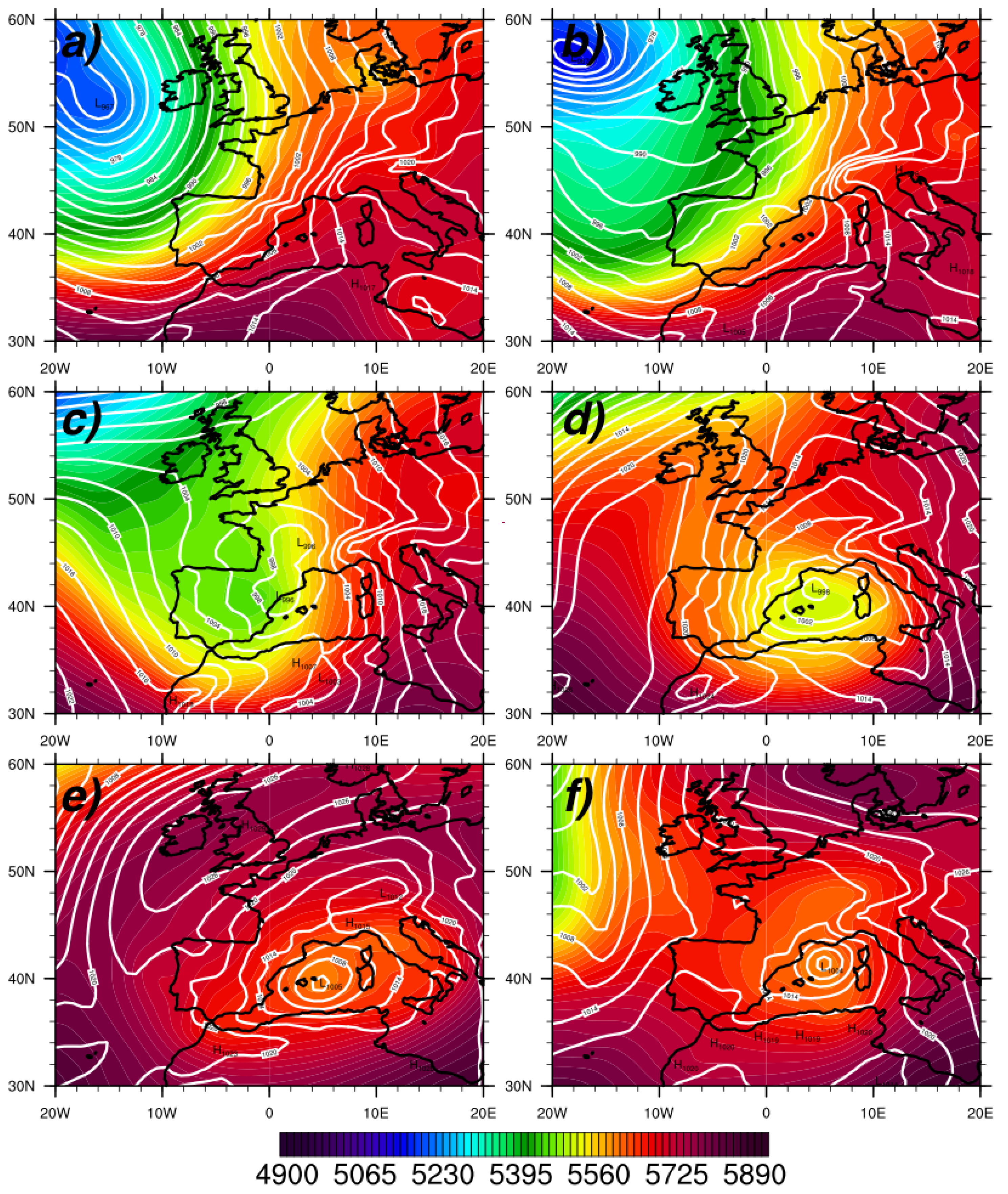
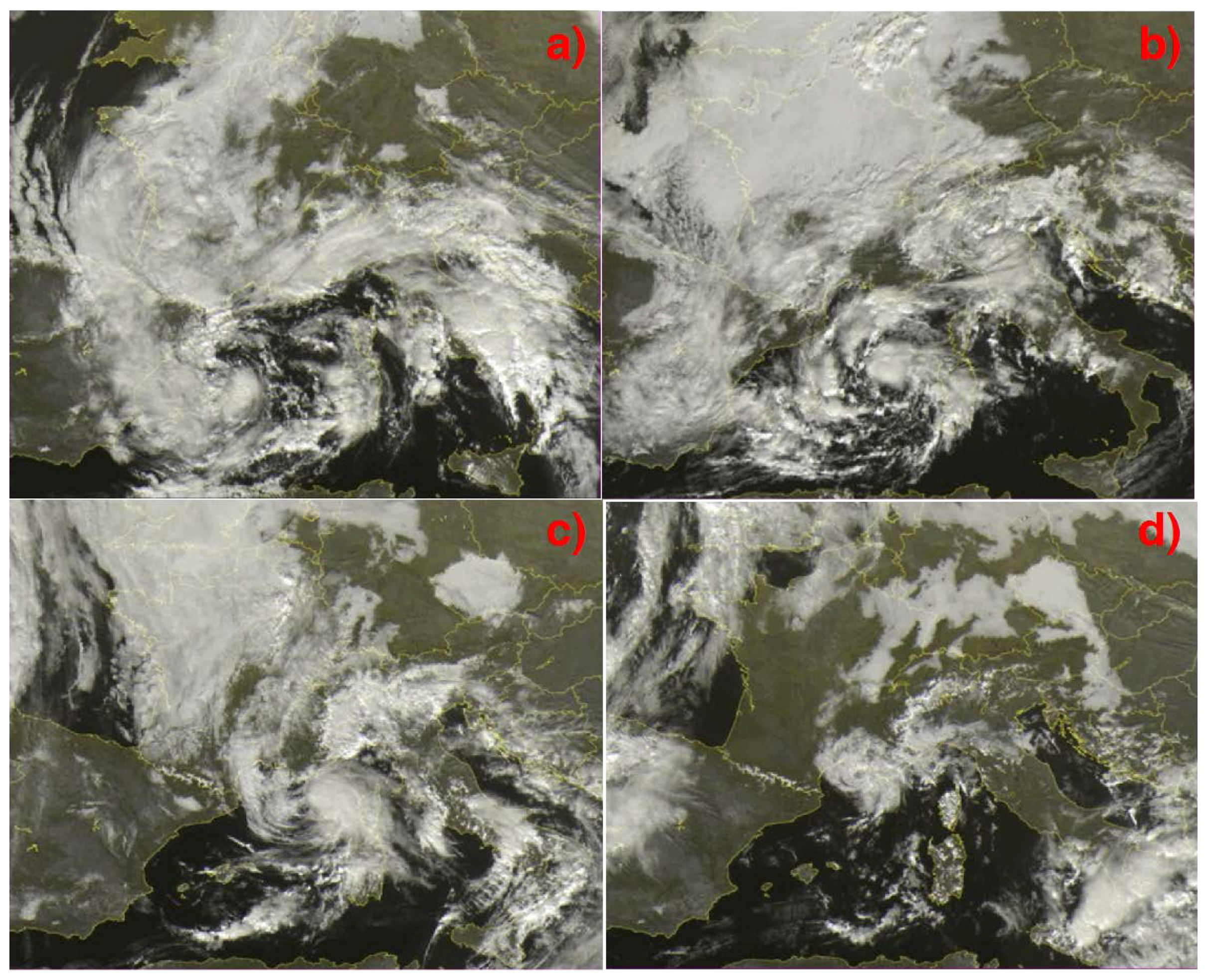
2. Case Study: Medicane ROLF

In this work, we study the TLC named ROLF (official name provided by the University of Berlin, the institution in charge to name the cyclones over the European area), selected as a “reference” case study among several events described in [4] due to the long persistence (more than 48 h) of its tropical features. ROLF developed from a cut-off low over Spain on 3 November 2011 [4], associated with a large and deep Atlantic depression centered to the west of England, while a high-pressure area affected eastern Europe (Figure 1 panel (a)). The Atlantic depression was “locked” between the high over central Europe and the Azores high. The meridional stretching of the Atlantic depression (Figure 1 panel (b)) induced the baroclinic wave to “cut-off” over the Gulf of Lion and to form a pressure minimum (on 6 November 2011 around 1000 hPa) (Figure 1 panel (c,d)). The depression was isolated from the synoptic circulation and was tilted with respect to the vertical axis, showing the typical characteristics of an extra-tropical cyclone [20]. On 7 November the pressure minima at sea level and at 500 hPa were aligned, e.g., the geopotential cut-off was located over the SLP (Sea Level Pressure) minimum (Figure 1 panel (e)), while the cyclone crossed the Balearic Islands and moved to the east (Figure 2 panels (a,b)). On the following day, it moved slowly northward towards the Gulf of Lion: in this phase, the TLC reached its highest intensity, with 10 m wind speed up to 30 m s⁻¹ and the lowest estimated pressure of around 985 hPa. Landfall occurred on 9 November (around 12 UTC) near the east coast of the Gulf of Lion (Figure 2 panel (d)). During this period, ROLF reached 10 m wind speeds of around 30 m s⁻¹, generated significant wave heights up to 8 m high, and a large rainfall amount, particularly in coastal areas.

Following [4], the estimated maximum wind speed at 900 hPa was approximately 46 m/s, the maximum radius was around 150 km and the phase with tropical characteristics lasted for approximately 2 days and half. As shown in Figure 3, the SST anomaly in the area of generation and transit of the Medicane was about +3 °C, and approximately +2 °C in the entire western Mediterranean basin, except from the coastal areas where some negative anomaly was recorded, mainly due to the intense coastal upwelling, which is very frequent in the area [21,22].

The Satellite Service Division of the National Oceanic and Atmospheric Administration (NOAA) carried out a preliminary analysis of the TLC [23], identifying its trajectory, estimating the minimum pressure and the maximum wind around the eye. This analysis was carried out during the event based on readily available data, aiming at a real-time assessment of the evolution of the TLC for operational purposes, but suffered from some inconsistencies as emerges from comparison with the ASCAT (Advanced SCATterometer) wind data (e.g., Figure 4). For this reason, in this work we estimated the trajectory of the cyclone by identifying the position of the eye, based on a set of georeferenced hourly-spaced satellite images (Eumetsat infrared datasets).

3. Numerical Modelling and Approach

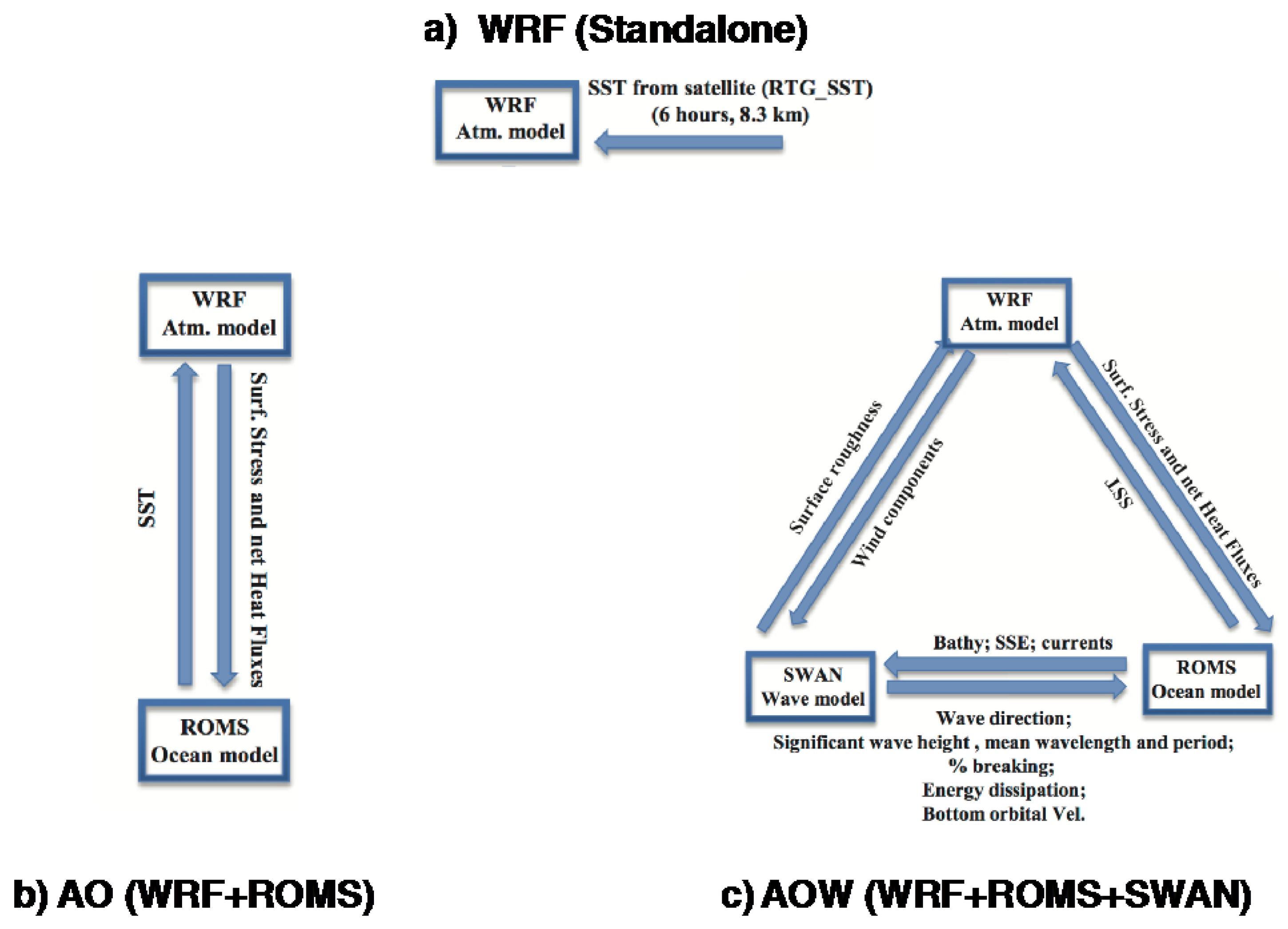
3.1. The COAWST Modeling Suite

COAWST is a complex system that manages different numerical models and allows feedbacks at the air-sea interface, through the interaction among SST, marine circulation, waves and atmospheric dynamics. The COAWST infrastructure is shown in Figure 5, where the models implemented in the system are represented: WRF for the atmosphere, ROMS for the ocean, and SWAN for the generation and propagation of wind waves.

In COAWST, the coupling is performed with the use of two tools responsible for the organization and communication of the information among different models. The tool that provides the data flow management is the Model Coupling Toolkit (MCT [26]), which is a dedicated library tool interfacing with the models, responsible for the exchange, transmission and processing of numerical data among the models using coupled and parallel approach by means of MPI libraries [27]. The exchange of variables takes place with a user-defined time step (300 s in this work). To allow the exchange of variables among the grids of the different models, COAWST relies on the Spherical Coordinate Remapping Interpolation Package (SCRIP [28]) to compute interpolation weights overcoming the possible differences in resolution, rotation and spatial coverage among the grids.

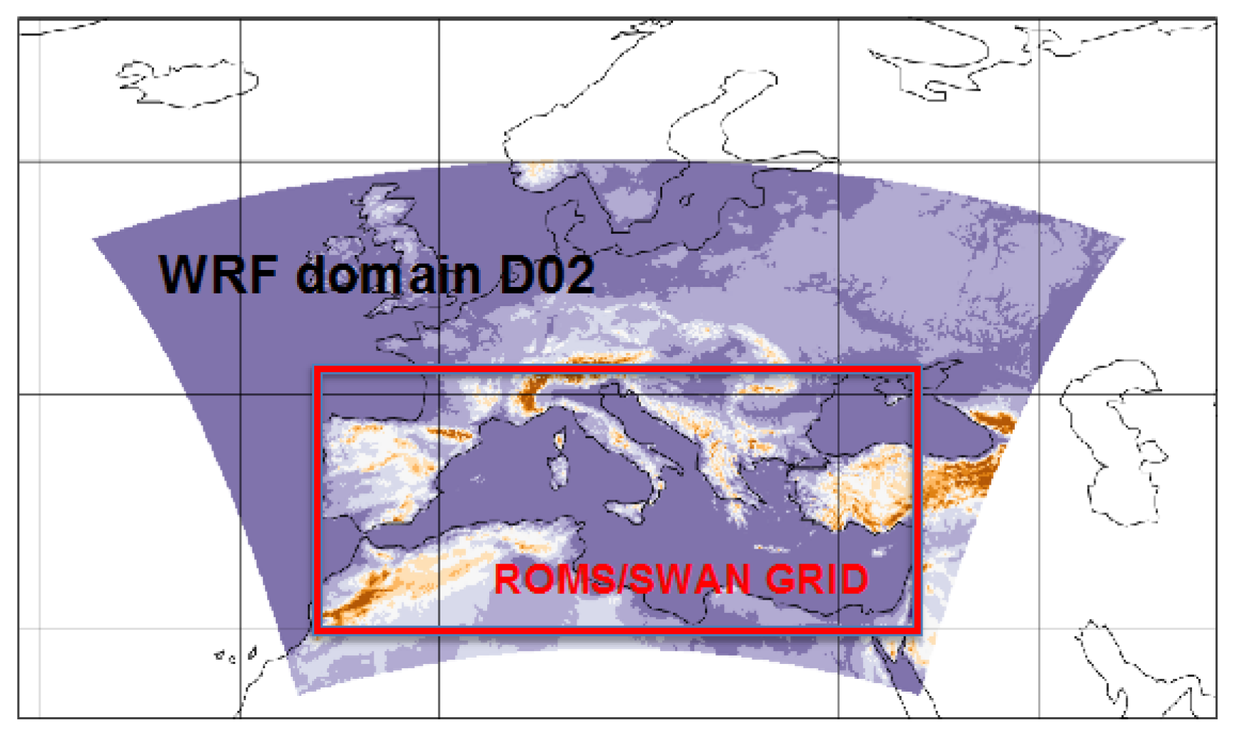
3.2. Atmospheric Model

WRF is a mesoscale numerical weather prediction model, serving a wide range of meteorological applications across scales from tens of meters to thousands of kilometers. WRF is a finite-difference numerical model over an Arakawa-C grid in σ (terrain-following) coordinate, fully compressible and non-hydrostatic [29].

The use of coupled models within COAWST requires that the atmospheric model domain fully encloses the ocean model grid, which in turn encompasses the whole Mediterranean basin. In addition, the need for a proper characterization of the large-scale dynamics, especially over the Atlantic Ocean, where the system comes from, led to the extension of the atmospheric model domain significantly to the west and north of the TLC position.

For these reasons, WRF is configured over a large “mother” grid with 350 × 250 points spaced by 25 × 25 km², centered at latitude 47.5° N and longitude 7.5° E, ranging from northern Norway to the Sahara Desert, and from the central Atlantic ocean to the western Caspian Sea. This grid provides the boundary conditions to a nested grid with 5 km horizontal spacing and 970 × 708 grid points, using a one-way nesting technique, ranging from the north-eastern Atlantic to the whole Mediterranean and Black Sea (Figure 6) with 55 vertical levels, the lowest one located 12 m above the ground. The topographic dataset is USGS (30′′ resolution on inner domain) interpolate, at the resolution of the grid.

3.3. Ocean Model

ROMS is a hydrostatic, finite differences, split-explicit, free-surface numerical model for ocean circulation and thermohaline processes [30]. It solves the RANS (Reynolds Average Navier-Stokes) equations in a horizontal Arakawa-C grid and s-coordinate (σ terrain-following coordinate is a special case of s-coordinate) in vertical [30,31,32]. In this work, we ran ROMS simulations over a grid with 5 km horizontal resolution (for consistency with the atmospheric model) and 30 vertical levels, using GEBCO bathymetry at 30′′. The grid has 532 × 264 grid points and covers the entire Mediterranean basin (Figure 6, red box) in order to prevent possible interpolation noise on an open sea boundary. The grid is closed at the Dardanelles and at the Strait of Gibraltar. As good practice, we ran a 15-day spin-up, initializing ROMS with MF-STEP fields retrieved from MyOcean (now CMEMS [33]) data referred to 20 October 2011 at 00:00 UTC. The spin-up was performed with the coupling technique between atmosphere and ocean (run AO, described further on) in order to achieve consistency with the dynamic atmospheric fields, with the use of the GFS-FNL dataset for initial and boundary conditions. In these simulations, ROMS used the Generic Length Scale mixing scheme as in [34].

3.4. Wave Model

The computation of wind wave dynamics in the Mediterranean Sea within the COAWST system relied on SWAN (Simulating WAves Nearshore), a third-generation wave model that computes wind-generated waves in offshore and coastal regions [35]. This model describes the generation, evolution and dissipation of the wave action variance density spectrum E(ω,θ), with ω the wave angular frequency, and θ the wave direction. SWAN solves a radiative time-dependent transport equation in E(ω,θ), accounting for the wind input, the wave-wave interactions, and several dissipation terms both in deep and shallow waters. From E(ω,θ), various wave parameters can then be estimated at any point of the computational domain. Typical output fields are the significant wave height, hereafter denoted as H_s, the peak and mean wave periods, and the mean wave propagation direction. In our simulations covering the whole Mediterranean Sea, we used a consolidated configuration for the coupled use of SWAN in the COAWST system, as discussed in [18,19,36,37]. In detail, SWAN has been implemented with the same horizontal resolution adopted for ROMS (in order to be coupled in COAWST, SWAN and ROMS models must use the same grid), being the wave action spectrum discretized with 36 equally spaced directions and 24 geometrically distributed frequencies f, such that f_n = f_n + 1/1.1, with f_n = 0.05 Hz. The SWAN model runs in non-stationary mode, namely with E(ω,θ) evolving in time, with a wind input from WRF every 300 s and the output saved every 3600 s.

3.5. Model Coupling in COAWST

As mentioned before, COAWST allows various levels of coupling among models, according to the degree of complexity in the implementation and the number of variables that are exchanged (as shown in Figure 5). The atmospheric model, the wave model and the ocean current model can then be mutually connected or excluded, as in the experiments described hereinafter.

3.5.1. WRF-Only Experiments

First, the simulations using WRF in standalone mode (WRF1-10 experiments, see

Table 1. Summary of all performed runs and their numerical setup. Acronyms used: CHA = Charnock [46]; OOST = Oost et al. [52]; TY: Taylor and Yelland et al. [49]; DRE: Drennan et al. [51]. MYI: Mellor-Yamada-Janjic’ [44]; MYNN: Mellor Yamada, as in [45].

Run Name	Coupl.	ROMS	SWAN	SST	Roughness	PBL	Initialization Time
WRF1–7	NO	NO	NO	RTG_SST	CHA	MYJ	4–7 November 2011, every 00 UTC and 12 UTC (7 runs)
WRF8	NO	NO	NO	RTG_SST	CHA	MYNN	6 November 2011 00 UTC
WRF9	NO	NO	NO	RTG_SST decrease by 3 °C	CHA	MYJ	6 November 2011 00 UTC
WRF10	NO	NO	NO	SST MFS System	CHA	MYJ	6 November 2011 00 UTC
AO1	YES	YES	NO	ROMS 5 km	CHA	MYJ	6 November 2011 00 UTC
AO2	YES	YES	NO	ROMS 5 km	CHA	MYNN	6 November 2011 00 UTC
AOW1	YES	YES	YES	ROMS 5 km	OOST	MYJ	6 November 2011 00UTC
AOW2	YES	YES	YES	ROMS 5 km	OOST	MYNN	6 November 2011 00 UTC
AOW3	YES	YES	YES	ROMS 5 km	TY	MYJ	6 November 2011 00 UTC
AOW4	YES	YES	YES	ROMS 5 km	DRE	MYJ	6 November 2011 00 UTC

and Figure 5 panel (a)), i.e., without any coupling to other models, are considered. As discussed in [19], the initial SST forcing can be represented in different ways. In this work, we have chosen the RTG_SST satellite dataset [38] available every 24 h with 8.3 km horizontal resolution. The configuration of the model in the control run is based on the same setup used in [4]. Kain-Fritsch formulation [39] was used for cumulus scheme, while Thompson scheme [40] was adopted for cloud physics and RRTMG [41] for short and long wave radiation schemes. Several dataset, among which NCEP reanalysis datasets [42], were tested. The initialization data was then choose of the standalone simulations are provided by the global model reanalyses GFS-FNL [43] (Final Reanalysis of the Global Forecasting System) with a resolution of 1° × 1°. The same data were used for the boundary conditions, updated every 6 h.

Seven simulations were performed using different initialization times (shifting the starting time every 12 h from 4 November, 00 UTC, to 7 November, 00 UTC) in order to test the sensitivity to the initial condition (run WRF1-7) and to identify the one leading to the best model performances. The role of the Planetary Boundary Layer (PBL) scheme is also analyzed, using both schemes available in COAWST (WRF5 and WRF8), namely “Mellor-Yamada-Janjic” MYJ [44] and Mellor-Yamada-Nakanishi-Niino MYNN2.5 [45], starting from the initial condition providing the best results (i.e., 00 UTC, 6 November—WRF5 and WRF8). All of these different configurations are shown in Table 1, for a total of 10 experiments using the WRF standalone configuration. The numerical formulation for surface roughness is taken from [46], used by default in WRF, with: z₀ = z_chu_*²/g, where z₀ is the roughness length, z_ch is the Charnock constant (0.0011), and u_* the friction velocity.

Also, since we speculate about the importance of the air-sea interactions in the development of the cyclone, the sensitivity to SST is analyzed by reducing the initial SST by 3 °C all over the domain in the control run (WRF9). In this way, the SST anomaly, present at moment of TLC formation, is removed and the experiment is performed with the average values of SST; the comparison of the two allows to disentangle the effect of a warmer sea surface. An additional run (WRF10) was forced using the same high-resolution SST provided by ROMS to initialize the coupled experiments (the boundary SST is also provided by the ROMS field every 6-h). This simulation bridges the conceptual gap between uncoupled and coupled runs and allows to discriminate the effects of coupling from the effect of using the same initial/boundary conditions without coupling.

3.5.2. AO (Atmosphere–Ocean Coupling) Experiments

The second set of simulations employs a two-way coupling of WRF and ROMS. In this configuration, the ROMS model sends the SST data to WRF every 300 s, while the WRF model uses the received SST data (Figure 5 panel (b)) as the boundary condition, and in turn sends the turbulent heat fluxes to ROMS (which does not need to recalculate them). The substantial difference between the WRF standalone case and the AO run is that in the latter, the SST provided by ROMS is at high resolution and updated frequently in a dynamically consistent way. In fact, the heat fluxes that WRF sends to ROMS are based on the SST that WRF receives from ROMS, therefore providing a consistent approach for energy and momentum [18,19,27,47]. In standalone configurations, the fluxes are calculated offline independently by the atmospheric and the ocean models, generating inconsistencies between the two representations. The surface roughness is parameterized using the Charnock algorithm in both models. As shown in Table 1, two different experiments are employed in the AO configuration, using respectively the MYJ (AO1 experiment) and MYNN 2.5 (AO2 experiment) PBL schemes. As in the standalone WRF case, we decided to use these two PBL calculation schemes because they are the only ones that implement the coupling with the wave in this COAWST version.

3.5.3. AOW (Atmosphere–Ocean–Wave Coupling) Experiments

The most complete COAWST coupling configuration includes the two-way interaction of air, ocean and wind waves, described by the exchange of information among the three different models: WRF, ROMS, SWAN (Figure 5 panel (c)). Differently from the case AO, the WRF model sends the wind components also to the SWAN wave model, that provides the wave parameters with which WRF calculates the surface roughness and the heat fluxes at the air-sea interface. ROMS and SWAN also communicate with each other, exchanging the components of the current along the water column and the wave parameters [15,36,48]. Two PBL schemes, widely used in the scientific community (MYJ and MYNN, mainly differing in their order of closure, respectively 1.5 and 2.5), are available in COAWST in its fully coupled configuration. Also, COAWST has the possibility to compute the surface roughness following 3 different formulations. The first one is TY, from a work by Taylor and Yelland [49], who proposed a wave steepness-dependent ocean roughness, relying on three datasets representing sea-state conditions ranging from strongly forced to shoaling [50]

$$\frac{z_0}{H_s}=1200{\left(\frac{u_{*}}{L_p}\right)}^{4.5}$$

(1)

where $z_0$ is the roughness length, L_p is the peak period and H_s is the significant wave height computed by SWAN. The scheme by Drennan [51], the DRE parameterization, uses a wave age-based formula for the ocean roughness:

$$\frac{z_0}{H_s}=3.35{\left(\frac{u_{*}}{C_p}\right)}^{3.4}$$

(2)

where C_p is the wave phase speed at the peak frequency and where $u_{*}$ is the friction velocity.

The OOST [52] parameterization is a wave-age dependent scheme based on the 1996 ASGAMAGE experiment, expressed as:

$$\frac{z_0}{L_p}=\frac{25.0}{\pi }{\left(\frac{u_{*}}{C_p}\right)}^{3.4}$$

(3)

To analyze the effect that the two PBL schemes and the three roughness formulations may have on the coupled model, a set of simulations is performed by changing the PBL and the surface roughness. The resulting experiments with the AOW configurations (two using respectively the MYJ-AOW1 run and MYNN-AOW2 run PBL schemes, and three varying the surface roughness—with the MYJ scheme-), are listed in Table 1.

4. Results

In this section we discuss the results of the sensitivity experiments to different initialization times, to the PBL scheme, to the type of coupling between the atmosphere, ocean and wave models; the effect of PBL schemes and of the roughness formulations in the case of coupling are analyzed separately. While a thorough investigation of the physical processes and their modeling characterization is left to a dedicated forthcoming paper, here we focus on some key quantities of interest for operational forecasting and emergency management, such as the trajectory and intensity of the pressure minimum, and the wind speed. In particular, the quality of modeled trajectories (retrieved following [53,54]) has been quantified in terms of geometrical distance from that retrieved from satellite data (Section 2, Figure 7 and Figure 8).

4.1. Uncoupled Simulation

4.1.1. Initialization Time

The first analysis aimed at identifying the most suitable initial time and at assessing the model sensitivity to this (runs WRF1-7 in Table 1). The trajectories in the runs initialized on 4 November 2011 are shown respectively in Figure 7 panel (a) (00:00 UTC) and in Figure 7 panel (b) (12:00 UTC).

The simulation starting at 00:00 UTC produces a shallow depression, which does not evolve into a TLC. The initialization at 12:00 UTC, 4 November (WRF2) also produces a weak depression in the early stage of the simulation, but the pressure minimum intensifies earlier, at about 09:00 UTC, 6 November, as shown in Figure 7 panel (b). The depression remains weak as the minimum pressure is generally above 1000 hPa (Figure 9 panel (a)), while the landfall occurs in the center of the Gulf of Lion, about 12 h before the observations. In this case, the average distance from the observed trajectory is 59 km (Table 1).

Figure 7 panels (c,d) show the trajectories produced by the WRF3/WRF4 runs, initialized respectively at 00:00 UTC and 12:00 UTC, 5 November. Both trajectories are rather far from the satellite-retrieved track (average distance respectively of 71 and 58 km); also, the run initialized at 00:00 UTC develops a pressure minimum of around 995 hPa, while the run initialized at 12:00 UTC produces a much deeper pressure minimum of 983 hPa (Figure 9 panel(a)). The depression generated by WRF3 fills-up over the sea, while the cyclone in the WRF4 does end up with a landfall, although its occurrence is anticipated by about 21 h compared to the observations.

Figure 7 panels (e,f) show the trajectories of the runs WRF5 and WRF6 initialized on 6 November respectively at 00:00 UTC (panel (e)) and at 12:00 UTC (panel (f)). These two simulations represent similar trajectories, which differ only in the last part of the TLC lifetime, but have different intensity during the entire evolution of the cyclone. In terms of trajectory, the run initialized at 00:00 UTC is slightly better, with an average distance of around 50 km, while for the other initializations we have a minimum distance of around 55–60 km (except for the WRF8 case, where the average distance is less than in WRF5 but the time evolution is anticipated compared to WRF5 and the observations). Also, the cyclone is more intense and reaches values of pressure minimum and wind speed very close to observations (Figure 9 panel (a)). On the other hand, the run initialized at 12:00 UTC has a better trajectory but does not deepen sufficiently and produce an unrealistically fast evolution of the TLC, in particular during the central part of the trajectory (Figure 9 panel (a). The simulation initialized at 00:00 UTC on 7 November (WRF7, Figure 7 panel (g)) provides the worst trajectory with an average distance of around the 90–100 km, and the depression does not reach pressure and wind speeds comparable with that provided by NOAA (Figure 9 panel (a,b)).

In conclusion, a significant sensitivity of the simulations to the initial condition is apparent both in terms of intensity and track. No simulation appears able to capture completely the observed evolution of the cyclone, in particular the timing in the central part of trajectory, when the cyclone makes a ring-like rotation addressing the difficulty in simulating correctly this category of events (see also [12,13,14]. Apparently, the most accurate simulations are those that do not start neither too early (when the cyclone is still developing and the model cannot capture the development processes of the storm) nor too late (since the model needs a spin-up time to downscale the low-resolution global model FNL data to high-resolution model simulations). In conclusion, the best runs start during the cyclone mature stage; among these, the best is WRF5.

4.1.2. PBL Scheme

Next, we compare the effect of two different schemes of PBL considering only the initialization time that produced the best results (WRF5 run). The PBL schemes are used to parameterize the unresolved vertical turbulent fluxes of heat and momentum in the lower levels of the atmosphere [54]. Results obtained when the PBL scheme is changed (WRF8 is implemented as run WRF5, initialized on 6 November at 00 UTC, but using MYNN2.5) are shown in Figure 7 panel (h) (blue line). The different PBL scheme does not lead to significant changes in the trajectories compared to WRF5 (red line), except from the last few hours, when the simulate trajectory is closer to the observed track near the landfall point. Comparing the two simulations, we note that the MYNN2.5 scheme generates a less intense cyclone in terms of pressure and wind speed (Figure 9 panels (c,d)). In conclusion, the advantage of using the updated MYNN scheme appears limited in the present case in terms of track, and even detrimental in terms of cyclone depth.

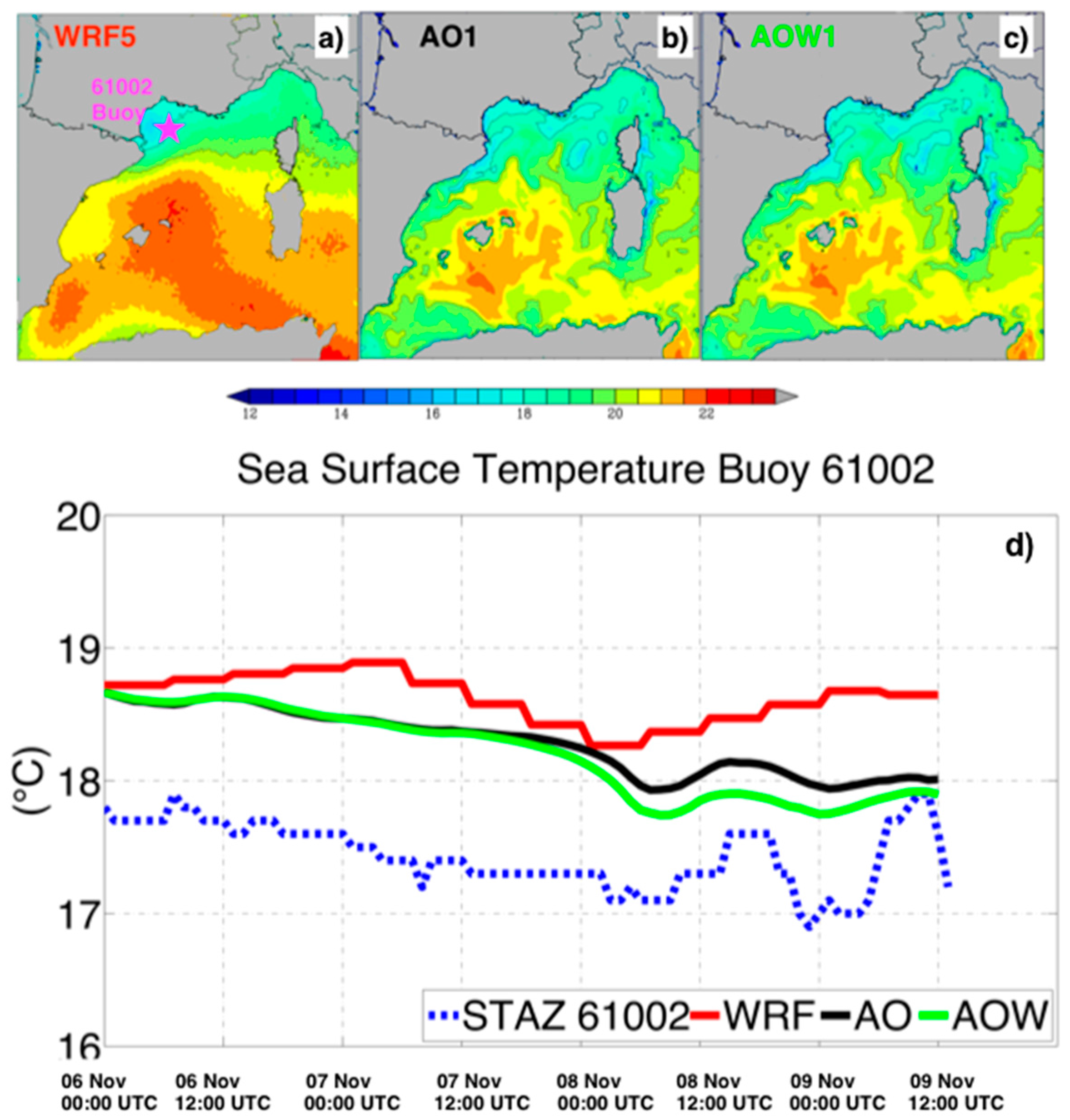
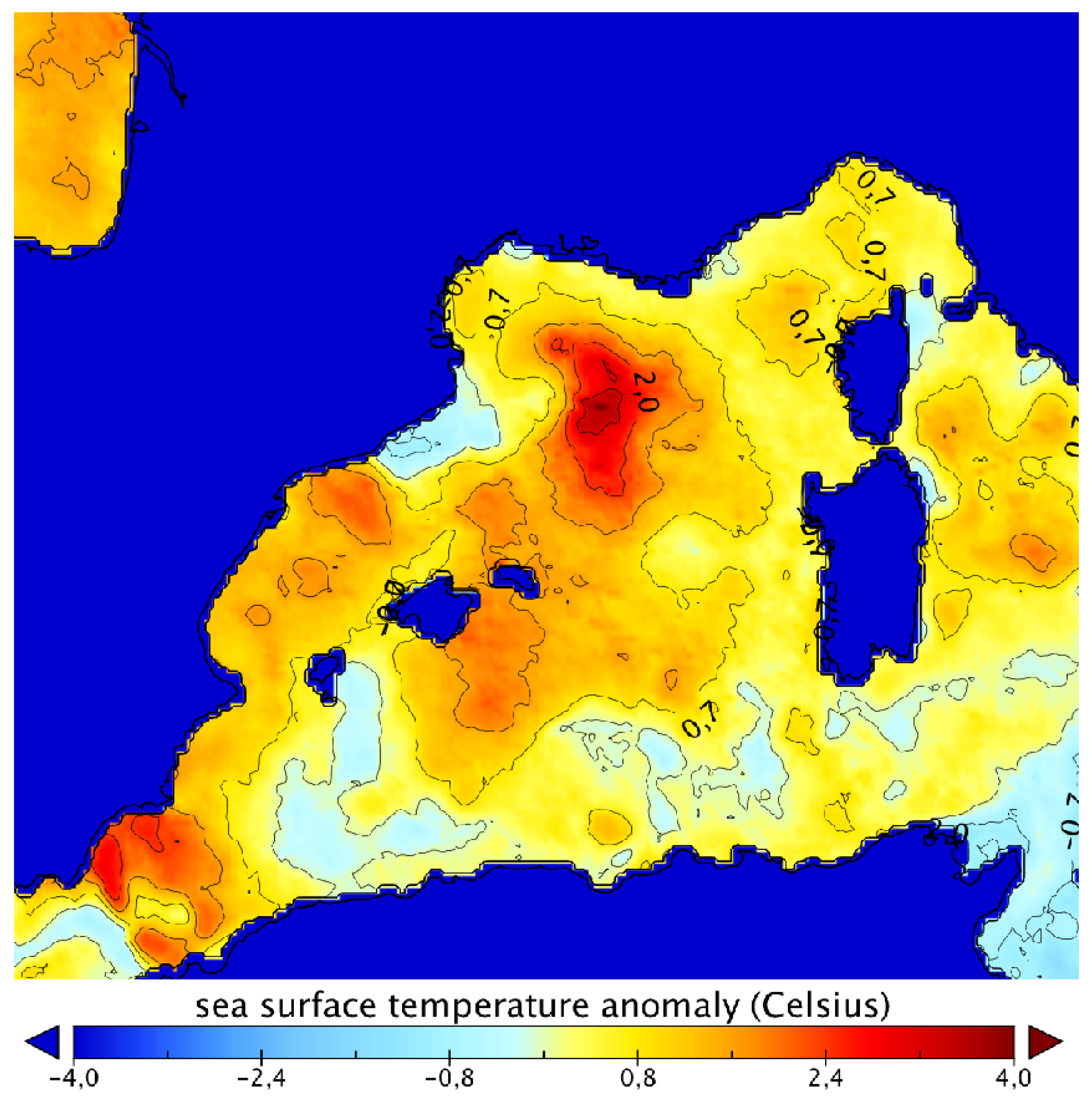
4.1.3. SST Variation

During the genesis of ROLF, the western Mediterranean sub-basin between the Balearic Islands, Sardinia and the Gulf of Lion was characterized by a SST anomaly of around +3 °C with respect to the climatology 1955–2004 produced by the Mediterranean forecasting System (MFS INGV, [24]) (Figure 3). Since the TLC ROLF was generated in this area, we decided to evaluate how relevant the observed anomaly of 3 °C may be for the cyclone generation and evolution, also in order to test the relevance of the sea surface fluxes for the cyclone development. To assess this, we decreased the SST by 3 °C, in a way similar to [10].

As shown in Figure 7 panel (i), the trajectory shows some variations, but it remains relatively close (around 50 km far) to that retrieved from satellite images. In the simulation WRF9 (where the SST was decreased by 3 °C), the pressure does not fall below 1000 hPa (Figure 9 panel (e)). As a consequence, during most of the simulation, the run WRF9 produces a less intense wind, by about 5 m/s, with respect to the run where the SST remained unchanged (Figure 9 panels (e,f)).

Finally, the same high-resolution SST provided by ROMS to initialize the coupled experiments (the boundary SST is also provided by the ROMS field every 6-h) is used in the experiment WRF10. This simulation provides a more detailed and physically consistent SST, but without coupling. The WRF10 experiment performance in terms of trajectory description is comparable to WRF5 (and, as will be shown, to the AO and AOW runs) (Figure 7 and Figure 8), although with a worse response in terms of geometrical distance (around 8 km worse compared to WRF5), and spatially characterized by a track covering a wider region.

4.2. Coupled Runs

The interaction between the atmosphere and the ocean takes place at their interface through heat and momentum fluxes. Fluxes are influenced respectively by the difference between SST and the air temperature, and by the surface roughness, which over the sea depends on the wave geometry. To explore the interaction among atmosphere-ocean-wave (runs AO and AOW), we chose as initialization time 00:00 UTC, 6 November 2011, the time of the best standalone simulation (WRF5). The 2-way coupling between the atmosphere and the ocean is activated first; next, we include also the wave dynamics. With these two coupled approaches, we explore the effect of SST and the effect of the waves on the energy exchanges. Both PBL schemes implemented in COAWST, i.e., MYJ and MYNN2.5, have been tested (see Table 1). The present experiments will also shed some light on the opportunity of using a coupled modeling system, not only for long simulation (as it is normally considered for climate simulations), but also over a short time range. The present cyclone, which persists over the sea for several hours, appears particularly attractive to address this issue.

4.2.1. PBL Scheme

Trajectories using the coupled system are shown in Figure 7 panel (m) (run AO1 and AOW1, for MYJ) and Figure 7 panel (l) (run AO2 and AOW2, for MYNN) and are compared with the results of the tests using the same implementation but in standalone configuration (WRF5 and WRF8). In the MYNN experiment panel (l), the effect of coupling is not significant in the early stages of the cyclone lifetime and is apparent only in the final phase of the storm, near the coast, where the trajectories in the coupled runs are directed westward and are closer to the observed track. However, the differences in the tracks are of the order of only 2–3 h and of about 50 km. The intensity of the TLC does not change significantly, being slightly weaker in the coupled simulations compared to the WRF standalone run in term of wind speed (Figure 9 panel (g)) and pressure (Figure 9 panel (h)).

The second set of coupled simulations was performed using the MYJ PBL parameterization. Even in this case, the tracks in the coupled runs (AO1 and AOW1) are directed more westward near landfall when compared to the run WRF5. This effect is more pronounced in AOW1, which also simulates a slightly slower cyclone especially in the central part of the track, likely related to the higher roughness in this run (not shown). Differently from the runs using the MYNN PBL, the cyclone is deeper in WRF5 and in AOW1 (Figure 9 panel (i)) reaching 987 hPa as pressure minimum than in run AO1 (pressure minimum of 990 hPa). To complete the comparison, Figure 10 presents pressure and wind speed for all the coupled runs retaining the same PBL scheme, but changing the roughness parameterization.

Going back to Figure 9, results obtained with MYJ appear more consistent with previous works (see for example, [55]) when compared to MYNN. In fact, the effects of the change in roughness appear to be properly transferred to the whole modeling system in the run AOW1: the higher roughness in AOW1 (Figure 11 panel (c) ) compared to WRF5 and AO1 runs (Figure 11 panels (a, b)), due to the inclusion of the waves in the calculation, produces higher fluxes and weaker winds than WRF5 (Figure 9 panel (l)) because of the increased drag, but deeper pressure minima than AO1 (Figure 9 panel (i)) because of higher amount of energy transferred to the atmosphere. Thus, in the following subsections, we will consider only the runs using the MYJ PBL scheme.

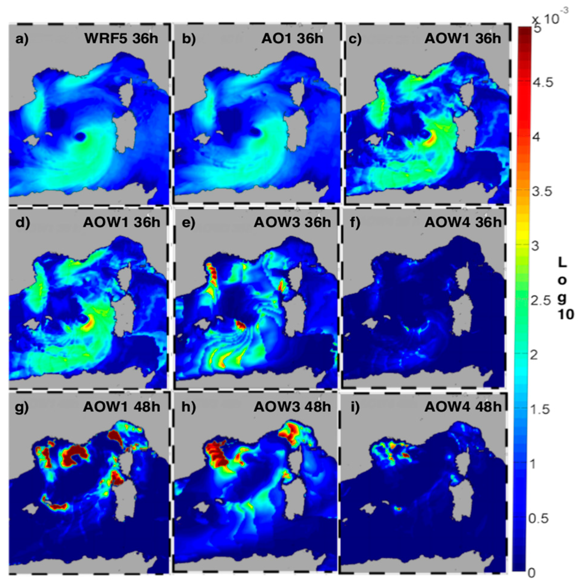
4.2.2. Surface Roughness Schemes

The effect of the surface roughness in the coupled runs using the MYJ PBL scheme is analyzed here. The heat fluxes are calculated with the surface roughness based on the geometric parameters calculated by the wave model SWAN. As mentioned above, the three schemes available in COAWST for parameterization of the surface roughness are: Oost (OOST), Taylor-Yelland (TY), and Drennan (DRE).

To better understand the effect of roughness, the results of the different modeling approaches used in this work are analyzed here. Figure 11 panels (a–c) show the surface roughness after 36 h of simulation, for the three runs WRF5, AO1, AOW1. Results for WRF5 and AO1 are similar since both use the [46] scheme for the calculation of roughness. Run AOW1 uses [52] and produces a higher roughness, in particular around the pressure minimum, where the waves are higher and steeper.

Panels (d–f) and (g–i) in Figure 11 show the surface roughness generated by the fully coupled runs, comparing the results for the different calculation schemes of roughness (Oost in AOW1, Taylor Yelland in AOW3, Drennan in AOW4). Results refer to 36 and 48 h of simulation, when the cyclone respectively reaches its maximum intensity and approaches the coast. The OOST scheme (AOW1) generates smaller roughness, giving rise to the maximum intensity in the neighborhood of the pressure minimum. The “discontinuous” distribution of the surface roughness in the other two schemes is due to the discretization of the peak frequencies (i.e., the frequency corresponding to the maximum energy component of the wave spectrum) that produce highly peaked periods. This depends on the spatial pattern variability of the wave-induced roughness and on the way the wave features are implemented within the OOST scheme. Indeed, since this scheme depends on wave age and the waves around the minimum are generally associated with a generative sea state, steeper waves (shorter period and greater height) can be expected, with greater influence in terms of roughness computation.

Figure 7 panel (n) shows that the trajectories of the cyclone in the simulations carried out with the three roughness schemes are close to each other, especially in the initial and central phase of the event, while some differences come out in the final stages of the cyclone lifetime (Figure 7 panel (l)). This divergence is probably caused by the highest difference in the surface roughness reached in the final part of the run, when the maximum wind intensity and significant wave height are simulated (not shown). After the cyclone begins to intensify, the run AOW1 (Figure 7 panel (n), red line) produces a much slower cyclone compared to the other two simulations. The distance between AOW1 and AOW3/AOW4 increases with time and reaches a maximum in the most intense phase of the cyclone.

Figure 11 panels (d–i) show that the highest roughness is produced by the OOST scheme (AOW1). This suggests that a higher roughness slows down the evolution of the cyclone, and slightly changes its trajectory (with an effect that increases with time); indeed, at the end of the simulation, the runs AOW3 and AOW4 are 6 h ahead compared to run AOW1. As shown in Figure 10 panel (a), the runs AOW3 and AOW4 show a cyclone with similar pressure minima, but less intense when compared to the run AOW1 (using OOST) by nearly 5 hPa. We speculate that this is due to the increased roughness in AOW1, which increases the heat fluxes and the energy available to the cyclone. However, the wind speed (Figure 10 panel (b)) is comparable in all the three runs in most of the lifetime (in some stages AOW1 produces the most intense wind speed), probably because the effect of the greater pressure gradient in run AOW1 is compensated by the more intense roughness around the eye of cyclone (Figure 10 panel (b)).

4.2.3. SST Analysis and Comparison

As described in [19,27,56], the way the SST is handled in coupled models plays a fundamental role in describing possible feedbacks between the atmosphere and ocean. In this work, we used different approaches. In most of the standalone runs (WRF1-9, therefore including WRF5 itself), the SST was provided by a low-resolution (8.3 km) radiometer, which may suffer from several errors due mainly to the limited resolution in coastal areas and to the observational holes caused by weather (cloudy) conditions (see for instance [18]). In the coupled runs, the ROMS model at 5 km resolution provides SST directly to the atmospheric model (whose wind in turn forces the oceanic circulation) after initialization by MFS modeled fields. Conceptually in the middle of these two approaches, MFS SST fields were also used as initial condition for WRF10 experiment, allowing to distinguish to what extent the results of AO and AOW runs actually depend on model coupling or they simply descend from the use of a different initial/boundary condition.

To evaluate the two different SST fields, we compare our results with the MeteoFrance #61002 buoy [57], located in the gulf of Lion. As shown in Figure 12 panels (a–c), spatial differences of SST between the standalone run and the coupled runs are significant for example in the Gulf of Lion, being the standalone run warmer by about 1–1.5 °C. In the sub-basin affected by the TLC, the SST of the standalone run is overestimated by about 2 °C (Figure 12 panels (a–c)). It is worth noting that the satellite data cannot reproduce coastal structures such as the coastal upwelling in the eastern Sardinia or the cold water circulating near the Catalan coast. A further confirmation comes from the analysis of the simulation results near the #61002 buoy, where the coupled run reproduces better the SST evolution compared to the standalone run. Despite that SST in the two approaches is initially similar, during the TLC evolution, only the coupled runs reduce the initial difference from the observation. During the passage of the TLC near the buoy, the run AOW1 further improves the model performance due to the effect of mixing induced by the waves (see also [58]). The decrease in SST is greater by about 0.1–0.3 °C compared to AO1 run, but it is too weak to affect significantly the development of the TLC. It is worth noting, although within a relatively narrow range of variation, the slight difference of WRF10 results from those of WRF5 and of the coupled runs (Figure 8) suggests that most of the features characterizing coupled experiments discussed so far are in fact mainly controlled by coupling instead of being the result of a different initial condition. On the other hand, Figure 9 shows that WRF10 and AO1 experiments produce comparable results in terms of timing and intensity of the cyclone.

5. Discussion and Conclusions

By means of a coupled atmosphere-ocean-wave modeling suite (COAWST), the goal of this work is to explore the sensitivity of the numerical simulation of Tropical Like Cyclone ROLF, by comparing trajectory, pressure and wind speed obtained using different levels of coupling and different numerical approaches. ROLF has been a particularly intense TLC and, throughout its lifetime, has caused extensive damage even considerably far away from its pressure minimum [59]. Indeed, the SST anomaly of about 3 °C in the central basin of the Balearic Islands (Figure 3) and the intensity and duration of the event allow consideration of ROLF as a paradigmatic case for disentangling the role of air-sea interactions on a cyclone evolution. Several studies have focused on the assessment of the SST role during TLC development. In particular, [9] showed how the use of more resolved and realistic SST fields (as in our case WRF10) with respect to the adoption of remotely sensed SST satellite fields with low spatial and temporal resolution (as our case WRF5) can play an important role to achieve better results in terms of trajectory and intensity of the cyclone. Other studies have focused on the identification of the physical factors that led to the formation and maintenance of this TLC [60]. In this study, we evaluate the sensitivity to initial conditions, resolution of the SST and to different levels of coupling, starting with a standalone WRF setup (with different initialization times), then employing a coupled atmospheric-ocean (AO) approach and finally a fully coupled implementation including waves (AOW). The effects of the PBL schemes in both uncoupled and coupled runs, as well as the effects of different surface roughness parameterization techniques, have been also explored.

The first set of results shows a strong sensitivity to the chosen initialization time (see also [12,13,14]). These tests confirmed that it is not sufficient to generally initialize the model close to the date of the event, but it is extremely important to explore which specific initialization produces the best result in terms of intensity and trajectory. When doing this, it is necessary to arrange a buffer time in which the PBL of the atmospheric model can settle down on the new SST structure that the satellite or the circulation model provide to the atmosphere. Furthermore, we observed that it is better to avoid a choice of initial conditions too close to the TLC spin-up period, to allow a proper adjustment. For this reason, we have chosen as the best initialization time 00:00 UTC on 6 November 2011, which provided good results in terms of trajectory and intensity. Following other examples [10], we also tested the decrease of SST over the whole domain, choosing to modify these conditions by 3 °C, since this is about the anomaly characterizing the Mediterranean basin near the cyclone on 8 November 2011. Finally, an uncoupled run initialized and forced with MFS SST was carried out, in order to investigate the effect of a high-resolution SST forcing without coupling before interpreting the results of coupled runs.

The resulting differences in terms of pressure minima show the importance of a correct distribution of the SST field, not only on the area affected by the phenomenon, but on the whole computational domain. The effect of SST reflects the different amount of energy transferred to the cyclone, and consequently its intensity (Figure 9 panels (e,f)). In addition, WRF10 experiment suggests that the implementation of an uncoupled model forced by a high-resolution SST can lead to modeled storm intensity not dissimilar to those produced by coupled models (in particular AO case). In addition, the strategy adopted in case WRF10, besides not being energetically consistent between sea and atmosphere, cannot be generally applied for operational purposes, since realistic SST forecasts are rarely available, while the easiest field estimates are provided by satellite data. This is also an indirect confirmation that in some cases it is therefore necessary to use a coupled approach, since in this case the temperature on the ocean side is then provided by a high-resolution circulation model and not by satellite images. As far as the effects of selected PBL are concerned, in the current COAWST release only the MYJ and MYNN2.5 schemes can be used when using the fully coupled atmosphere-ocean-wave model setup. We therefore performed a comparison among the standalone WRF model and the coupled runs (experiments WRF8-AO2-AOW2, WRF5-AO1-AOW1). The comparison shows that a change of the PBL scheme slightly affects the trajectory in the early and middle part of the run, but that this modification becomes larger in the final part, when the TLC approaches the coast. Indeed, the two PBL schemes have limited effects when the cyclone moves over the sea, and probably the different interactions between the atmosphere and the ocean due to the different distribution of SST fields take several hours to develop across the atmosphere. More specifically, looking at Figure 8 it can be seen that the total geometric distances obtained by the two runs using different PBL schemes are comparable; however, the difference increases when the TLC approaches the coast, and this can also explain the slight discrepancy resulting in the final landfall timing.

We can further discuss the most significant differences in terms of intensity. As shown in the Figure 9 panels (g–l), run WRF5 produces a cyclone that is always more intense with respect to that produced by the coupled runs, because the satellite SST data are slightly warmer than the ROMS modeled surface temperature, and this produces an intensive development by approximately 5 hPa.

In this case the choice of the PBL scheme becomes also crucial, as the PBL MYJ generates more intense heat fluxes (not shown) with respect to the MYNN2.5 scheme. We have therefore chosen the run with MYJ PBL as control run.

In the coupled runs, differences emerge especially with the use of MYJ PBL. In this case, the run AOW1 is more intense than run AO1 (Figure 9 panels (i,l)) only in terms of atmospheric pressure and not in wind speeds. This could be attributed to the effect of the surface roughness calculated with the OOST scheme in run AOW1. This choice indeed generates a larger roughness around the pressure minimum (Figure 11 panels (a–c)), which induces an increase in the fluxes leading to an intense development of the cyclone, similarly to what WRF5 run produced (where higher SST generated intense heat fluxes). The higher surface roughness also increases friction and, therefore, tends to limit the intensification of the 10m wind, as shown in Figure 9 panel (i). Moreover, the parameterization scheme adopted for the surface roughness has another crucial role, as shown in both Figure 10 and Figure 11; among these schemes, the one that performs better is OOST (see Figure 8), which generates a consistent and homogeneous surface roughness, if compared with other simulations that use the Charnock scheme.

Figure 12 helps us to understand how the use of coupled models can turn out to be important also on the oceanographic side. The SST data in Figure 12 panels (a–c) show the differences in the analysis among the WRF5, AO1, AOW1 runs, while panel (d) shows a temperature time series for the three models compared to data provided by the close by MeteoFrance buoy #61002. Results clearly show that the spectro-radiometer overestimates the SST especially in areas close to the coast, where the cloudiness effect is greater; also because of the low resolution of the satellite, the meandering and small-scale structures are not resolved. Further, by comparing runs AO1 and AOW1, it can be seen that in the latter the wave mixing effects induce a larger cooling of the sea surface [18,58].

Generally speaking then, at least in this specific TLC case the use of coupled models improved the reliability of the results in terms of heat and momentum fluxes [18,19], which are more consistent thanks to a better description of the SST fields. Also, in this specific study, the TLC was shown to be more sensitive to the initialization than to the coupling strategy. Considering the fundamental role played by the roughness parameterization and the PBL scheme, we suggest to select them on the basis of specific tests, given that the responses may be very different depending on the phenomena and the type of waves that generate the roughness. Last but not least, as already mentioned, if it is true that the use of coupled models strategy can be beneficial for modeling TLCs, it should be recalled that it also leads to an increase of complexity on the informatics side. In addition to this, model coupling may emphasize some problems typical in all numerical approaches, such as the sensitivity to boundary conditions in atmospheric models (especially when dealing with temperature and soil type). In particular, it should be reminded that the SST fields must be prescribed very carefully, since they may be significantly different from that originally used in the global model adopted to produce the initialization. As a final remark, a critical aspect is represented also by the initialization time of the TLC where possible help may be sought for in-variational assimilation techniques (3Dvar-4Dvar), although care must be taken in approaches (e.g., “hotstart”) that have to be shared by all the employed models.

References

1. Ernst, J.A.; Matson, M. A Mediterranean Tropical Storm? Weather 1983, 38, 332–337. [Google Scholar] [CrossRef]
2. Moscatello, A.; Miglietta, M.M.; Rotunno, R. Observational Analysis of a Mediterranean “Hurricane” over Southeastern Italy. Weather 2008, 63, 306–311. [Google Scholar] [CrossRef]
3. Akhtar, N.; Brauch, J.; Dobler, A.; Béranger, K.; Ahrens, B. Medicanes in an ocean—Atmosphere coupled regional climate model. Nat. Hazards Earth Syst. Sci. 2014, 14, 2189–2201. [Google Scholar] [CrossRef]
4. Miglietta, M.M.; Laviola, S.; Malvaldi, A.; Conte, D.; Levizzani, V.; Price, C. Analysis of tropical-like cyclones over the Mediterranean Sea through a combined modeling and satellite approach. Geophys. Res. Lett. 2013, 40, 2400–2405. [Google Scholar] [CrossRef]
5. Cavicchia, L.; von Storch, H. The simulation of medicanes in a high-resolution regional climate model. Clim. Dyn. 2012, 39, 2273–2290. [Google Scholar] [CrossRef]
6. Tous, M.; Romero, R. Meteorological environments associated with medicane development. Int. J. Climatol. 2013, 33, 1–14. [Google Scholar] [CrossRef]
7. Emanuel, K. Genesis and maintenance of “Mediterranean hurricanes”. Adv. Geosci. 2005, 2, 217–220. [Google Scholar] [CrossRef]
8. Fita, L.; Romero, R.; Luque, A.; Emanuel, K.; Ramis, C. Analysis of the environments of seven Mediterranean tropical-like storms using an axisymmetric, nonhydrostatic, cloud resolving model. Nat. Hazards Earth Syst. Sci. 2007, 7, 41–56. [Google Scholar] [CrossRef]
9. Cioni, G.; Malguzzi, P.; Buzzi, A. Thermal structure and dynamical precursor of a Mediterranean tropical-like cyclone. Q. J. R. Meteorol. Soc. 2016, 142, 1757–1766. [Google Scholar] [CrossRef]
10. Miglietta, M.M.; Moscatello, A.; Conte, D.; Mannarini, G.; Lacorata, G.; Rotunno, R. Numerical analysis of a Mediterranean “hurricane” over south-eastern Italy: Sensitivity experiments to sea surface temperature. Atmos. Res. 2011, 101, 412–426. [Google Scholar] [CrossRef]
11. Moscatello, A.; Miglietta, M.M.; Rotunno, R. Numerical Analysis of a Mediterranean “Hurricane” over Southeastern Italy. Mon. Weather Rev. 2008, 136, 4373–4397. [Google Scholar] [CrossRef]
12. Davolio, S.; Miglietta, M.M.; Moscatello, A.; Pacifico, F.; Buzzi, A.; Rotunno, R. Numerical forecast and analysis of a tropical-like cyclone in the Ionian Sea. Nat. Hazards Earth Syst. Sci. 2009, 9, 551–562. [Google Scholar] [CrossRef]
13. Chaboureau, J.-P.; Pantillon, F.; Lambert, D.; Richard, E.; Claud, C. Tropical transition of a Mediterranean storm by jet crossing. Q. J. R. Meteorol. Soc. 2012, 138, 596–611. [Google Scholar] [CrossRef]
14. Miglietta, M.M.; Mastrangelo, D.; Conte, D. Influence of physics parameterization schemes on the simulation of a tropical-like cyclone in the Mediterranean Sea. Atmos. Res. 2015, 153, 360–375. [Google Scholar] [CrossRef]
15. Warner, J.C.; Armstrong, B.; He, R.; Zambon, J.B. Development of a Coupled Ocean-Atmosphere-Wave-Sediment Transport (COAWST) Modeling System. Ocean Model. 2010, 35, 230–244. [Google Scholar] [CrossRef]
16. Olabarrieta, M.; Warner, J.C.; Armstrong, B.; Zambon, J.B.; He, R. Ocean-atmosphere dynamics during Hurricane Ida and Nor’Ida: An application of the coupled ocean-atmosphere-wave-sediment transport (COAWST) modeling system. Ocean Model. 2012, 43, 112–137. [Google Scholar] [CrossRef]
17. Zambon, J.B.; He, R.; Warner, J.C. Investigation of hurricane Ivan using the coupled ocean-atmosphere-wave-sediment transport (COAWST) model. Ocean Dyn. 2014, 64, 1535–1554. [Google Scholar] [CrossRef]
18. Carniel, S.; Benetazzo, A.; Bonaldo, D.; Falcieri, F.M.; Miglietta, M.M.; Ricchi, A.; Sclavo, M. Scratching beneath the surface while coupling atmosphere, ocean and waves: Analysis of a dense water formation event. Ocean Model. 2016, 101, 101–112. [Google Scholar] [CrossRef]
19. Ricchi, A.; Miglietta, M.M.; Falco, P.P.; Benetazzo, A.; Bonaldo, D.; Bergamasco, A.; Sclavo, M.; Carniel, S. On the use of a coupled ocean-atmosphere-wave model during an extreme cold air outbreak over the Adriatic Sea. Atmos. Res. 2016, 172, 48–65. [Google Scholar] [CrossRef]
20. Hart, R.E. A Cyclone Phase Space Derived from Thermal Wind and Thermal Asymmetry. Mon. Weather Rev. 2003, 131, 585–616. [Google Scholar] [CrossRef]
21. Millot, C. Circulation in the Western Mediterranean Sea. J. Mar. Syst. 1999, 20, 423–442. [Google Scholar] [CrossRef]
22. Renault, L.; Oguz, T.; Pascual, A.; Vizoso, G.; Tintore, J. Surface circulation in the Alborán Sea (western Mediterranean) inferred from remotely sensed data. J. Geophys. Res. Oceans 2012, 117. [Google Scholar] [CrossRef]
23. NOAA National Oceanic and Atmospheric Administration. NESDIS National Environmental Satellite, Data and Information Service). Tropical Bulletin Archive. 2011. Available online: http://www.ssd.noaa.gov/PS/TROP/2011/bulletin/archive.html (accessed on 15 January 2016).
24. Pinardi, N.; Allen, I.; Demirov, E.; Mey, P.D.; Korres, G.; Lascaratos, A.; Traon, P.L.; Maillard, C. Annales Geophysicae The Mediterranean ocean forecasting system: First phase of implementation (1998–2001). Ann. Geophys. 2003, 21, 3–20. [Google Scholar] [CrossRef]
25. Oddo, P.; Adani, M.; Pinardi, N.; Fratianni, C.; Tonani, M.; Pettenuzzo, D. A nested Atlantic-Mediterranean Sea general circulation model for operational forecasting. Ocean Sci. 2009, 5, 461–473. [Google Scholar] [CrossRef]
26. Larson, J.; Jacob, R.; Ong, E. The Model Coupling Toolkit: A New Fortran90 Toolkit for Building Multiphysics Parallel Coupled Models. Int. J. High Perform. Comput. Appl. 2005, 19, 277–292. [Google Scholar] [CrossRef]
27. Warner, J.C.; Sherwood, C.R.; Signell, R.P.; Harris, C.K.; Arango, H.G. Development of a three-dimensional, regional, coupled wave, current, and sediment-transport model. Comput. Geosci. 2008, 34, 1284–1306. [Google Scholar] [CrossRef]
28. Jones, P.W. SCRIP Manual. 1999. Available online: oceans11.lanl.gov/svn/SCRIP/trunk/SCRIP/doc/SCRIPusers.pdf (accessed on 20 October 2016).
29. Skamarock, W.C.; Klemp, J.B. A time-split nonhydrostatic atmospheric model for weather research and forecasting applications. J. Comput. Phys. 2008, 227, 3465–3485. [Google Scholar] [CrossRef]
30. Shchepetkin, A.F.; McWilliams, J.C. The regional oceanic modeling system (ROMS): A split-explicit, free-surface, topography-following-coordinate oceanic model. Ocean Model. 2005, 9, 347–404. [Google Scholar] [CrossRef]
31. Shchepetkin, A.F.; McWilliams, J.C. Computational Kernel Algorithms for Fine-Scale, Multiprocess, Longtime Oceanic Simulations. In Handbook of Numerical Analysis; Elsevier: Oxford, UK, 2009; pp. 121–183. [Google Scholar]
32. Haidvogel, D.B.; Arango, H.; Budgell, W.P.; Cornuelle, B.D.; Curchitser, E.; Di Lorenzo, E.; Fennel, K.; Geyer, W.R.; Hermann, A.J.; Lanerolle, L.; et al. Ocean forecasting in terrain-following coordinates: Formulation and skill assessment of the Regional Ocean Modeling System. J. Comput. Phys. 2008, 227, 3595–3624. [Google Scholar] [CrossRef]
33. Copernicus Marine Environment Monitoring Service (CMEMS). Mediterranean Sea Physics Reanalysis Model. Available online: http://marine.copernicus.eu (accessed on 10 January 2016).
34. Carniel, S.; Warner, J.C.; Chiggiato, J.; Sclavo, M. Investigating the impact of surface wave breaking on modeling the trajectories of drifters in the northern Adriatic Sea during a wind-storm event. Ocean Model. 2009, 30, 225–239. [Google Scholar] [CrossRef]
35. Booij, N.; Ris, R.C.; Holthuijsen, L.H. A third-generation wave model for coastal regions: 1. Model description and validation. J. Geophys. Res. Ocean. 1999, 104, 7649–7666. [Google Scholar] [CrossRef]
36. Benetazzo, A.; Fedele, F.; Carniel, S.; Ricchi, A.; Bucchignani, E.; Sclavo, M. Wave climate of the Adriatic Sea: A future scenario simulation. Nat. Hazards Earth Syst. Sci. 2012, 12, 2065–2076. [Google Scholar] [CrossRef]
37. Benetazzo, A.; Bergamasco, A.; Bonaldo, D.; Falcieri, F.M.; Sclavo, M.; Langone, L.; Carniel, S. Response of the Adriatic Sea to an intense cold air outbreak: Dense water dynamics and wave-induced transport. Prog. Oceanogr. 2014, 128, 115–138. [Google Scholar] [CrossRef]
38. Gemmill, W.; Katz, B.; Li, X. Daily Real-Time, Global Sea Surface Temperature, High-Resolution Analysis: RTG_SST_HR; NOAA/NWS/NCEP/MMAB Office Note; National Centers for Environmental Prediction: Camp Springs, MD, USA, 2007; p. 39. [Google Scholar]
39. Kain, J.S. The Kain-Fritsch Convective Parameterization: An Update. J. Appl. Meteorol. 2004, 43, 170–181. [Google Scholar] [CrossRef]
40. Thompson, G.; Field, P.R.; Rasmussen, R.M.; Hall, W.D. Explicit Forecasts of Winter Precipitation Using an Improved Bulk Microphysics Scheme. Part II: Implementation of a New Snow Parameterization. Mon. Weather Rev. 2008, 136, 5095–5115. [Google Scholar] [CrossRef]
41. Mlawer, E.J.; Taubman, S.J.; Brown, P.D.; Iacono, M.J.; Clough, S.A. Radiative transfer for inhomogeneous atmospheres: RRTM, a validated correlated-k model for the longwave. J. Geophys. Res. 1997, 102. [Google Scholar] [CrossRef]
42. Compo, G.P.; Whitaker, J.S.; Sardeshmukh, P.D.; Matsui, N.; Allan, R.J.; Yin, X.; Gleason, B.E.; Vose, R.S.; Rutledge, G.; Bessemoulin, P.; et al. The Twentieth Century Reanalysis Project. Q. J. R. Meteorol. Soc. 2011, 137, 1–28. [Google Scholar] [CrossRef]
43. NOAA National Oceanic and Atmospheric Administration; National Centers for Environmental Information. GFS-FNL (Final Reanalysis of the Global Forecasting System). Available online: https://www.ncdc.noaa.gov/data-access/model-data/model-datasets/global-forcast-system-gfs (accessed on 10 January 2016).
44. Janjić, Z.I. The Step-Mountain Eta Coordinate Model: Further Developments of the Convection, Viscous Sublayer, and Turbulence Closure Schemes. Mon. Weather Rev. 1994. [Google Scholar] [CrossRef]
45. Nakanishi, M.; Niino, H. An Improved Mellor–Yamada Level-3 Model: Its Numerical Stability and Application to a Regional Prediction of Advection Fog. Bound.-Layer Meteorol. 2006, 119, 397–407. [Google Scholar] [CrossRef]
46. Charnock, H. Wind stress on a water surface. Q. J. R. Meteorol. Soc. 1955, 81, 639–640. [Google Scholar] [CrossRef]
47. Small, R.J.; Campbell, T.; Teixeira, J.; Carniel, S.; Smith, T.A.; Dykes, J.; Chen, S.; Allard, R. Air-Sea Interaction in the Ligurian Sea: Assessment of a Coupled Ocean-Atmosphere Model Using In Situ Data from LASIE07. Mon. Weather Rev. 2011, 139, 1785–1808. [Google Scholar] [CrossRef]
48. Kumar, N.; Voulgaris, G.; Warner, J.C.; Olabarrieta, M. Implementation of the vortex force formalism in the coupled ocean-atmosphere-wave-sediment transport (COAWST) modeling system for inner shelf and surf zone applications. Ocean Model. 2012, 47, 65–95. [Google Scholar] [CrossRef]
49. Taylor, P.K.; Yelland, M.J. The Dependence of Sea Surface Roughness on the Height and Steepness of the Waves. J. Phys. Oceanogr. 2001. [Google Scholar] [CrossRef]
50. Olabarrieta, M.; Medina, R.; Castanedo, S. Effects of wave-current interaction on the current profile. Coast. Eng. 2010, 57, 643–655. [Google Scholar] [CrossRef]
51. Drennan, W.M.; Graber, H.C.; Hauser, D.; Quentin, C. On the wave age dependence of wind stress over pure wind seas. J. Geophys. Res. 2003, 108, 8062. [Google Scholar] [CrossRef]
52. Oost, W.A.; Komen, G.J.; Jacobs, C.M.J.; Van Oort, C. New evidence for a relation between wind stress and wave age from measurements during ASGAMAGE. Bound.-Layer Meteorol. 2002, 103, 409–438. [Google Scholar] [CrossRef]
53. Picornell, M.A.; Carrassi, N.A.; Jansá, A. A study on the forecast quality of the mediterranean cyclones. In Proceedings of the 4th EGS Plinius Conference, Mallorca, Spain, 2–4 October 2002. [Google Scholar]
54. Hu, X.-M.; Nielsen-Gammon, J.W.; Zhang, F. Evaluation of Three Planetary Boundary Layer Schemes in the WRF Model. JAMC 2010. [Google Scholar] [CrossRef]
55. Renault, L.; Chiggiato, J.; Warner, J.C.; Gomez, M.; Vizoso, G.; Tintoré, J. Coupled atmosphere-ocean-wave simulations of a storm event over the Gulf of Lion and Balearic Sea. J. Geophys. Res. Oceans 2012, 117. [Google Scholar] [CrossRef]
56. Davolio, S.; Stocchi, P.; Benetazzo, A.; Bohm, E.; Riminucci, F.; Ravaioli, M.; Li, X.-M.; Carniel, S. Exceptional Bora outbreak in winter 2012: Validation and analysis of high-resolution atmospheric model simulations in the northern Adriatic area. Dyn. Atmos. Oceans 2015, 71, 1–20. [Google Scholar] [CrossRef]
57. NOAA National Oceanic and Atmospheric Administration, Nationa Data Buoy Center. Station 61002, Meteorological ad Waves Buoy Owned and Maintained by “Meteo France”. Available online: http://www.ndbc.noaa.gov/station_page.php?station=61002 (accessed on 15 January 2016).
58. Benetazzo, A.; Carniel, S.; Sclavo, M.; Bergamasco, A. Wave-current interaction: Effect on the wave field in a semi-enclosed basin. Ocean Model. 2013, 70, 152–165. [Google Scholar] [CrossRef]
59. Cassola, F.; Ferrari, F.; Mazzino, A.; Miglietta, M.M. The role of the sea on the flsh floods events over Liguria (Italy). Geophys. Res. Lett. 2016, 43, 3534–3542. [Google Scholar] [CrossRef]
60. Miglietta, M.M.; Cerrai, D.; Laviola, S.; Cattani, E.; Levizzani, V. Potential vorticity patterns in Mediterranean “hurricanes”. Geophys. Res. Lett. 2017. [Google Scholar] [CrossRef]
Figure 1. Snapshots of surface pressure (white lines; c.i. = 3 hPa), and 500 hPa geopotential height (colors) on 3 November 2011, 00 UTC (panel (a)) and 4 November 2011, 00 UTC (panel (b))—during the transit of the Atlantic baroclinic wave over Spain, close to the Balearic Sea-, 5 November 2011, 00:00 UTC (panel (c))—during the formation of the ROLF depression over Spain-, on 6 November 2011, 00:00 UTC (panel (d))—during the cut-off low over the Balearic sea-, on 7 November 2011, 00:00 UTC (panel (e)) and 8 November 2011, 00:00 UTC (panel (f)). Data are from ECMWF ERA-40 (European Center for Medium range Weather Forecasting).
Atmosphere 08 00092 g001
Figure 2. Visible channel of Meteosat Satellite images on 6 November 2011, 12:00 UTC (panel (a)), 7 November 2011, 12:00 UTC (panel (b)), 8 November 2011, 12:00 UTC (panel (c)) and 9 November 2011, 12:00 UTC (panel (d)) (source: www.sat24.com; copyright: EUMETSAT). In panel (a) we can see the formation of the TLC, whereas in the panel (b) the TLC is formed and in panel (c) ROLF is still well identified. In panel (d) the landfall of cyclone is shown.
Atmosphere 08 00092 g002
Figure 3. SST anomaly produced by the Mediterranean Forecasting System (MFS INGV, [24]) on 8 November 2011, consisting of the difference between analysed SST from MFS and the climatology 1955–2004 supplied by the Nucleus for European Modelling of the Ocean (NEMO), with a variational data assimilation scheme (OceanVAR) for temperature and salinity vertical profiles and satellite Sea Level Anomaly along track data. The model horizontal grid resolution is 1°/16° (ca. 6–7 km) and the unevenly spaced vertical levels are 72 [25]. In this figure, we can see the positive SST anomaly in the western Mediterranean Sea, between 1–3.7 °C, in particular over the formation area of the TLC.
Atmosphere 08 00092 g003
Figure 4. Wind speed and direction from the Advanced Scatterometer Wind data (ASCAT) shown on 8 November 10:00 UTC at 25 km of resolution. In the proximity of the pressure minimum, wind speed is approximately 25–28 ms−1 (50–55 knots). The area with maximum intensity is located on the northern side of TLC.
Atmosphere 08 00092 g004
Figure 5. The three different configurations adopted in this study. Panel (a): WRF run: atmosphere standalone (WRF uses the SST data from the RTG_SST dataset, every 6 h). Panel (b): AO (Atmosphere-Ocean) run: coupling between atmosphere and ocean (WRF receives the SST from ROMS model, at 1 km resolution, every 300 s, and exchanges the turbulent heat fluxes with ROMS). Panel (c): AOW (Atmosphere–Ocean–Wave) run: full atmosphere-ocean-wave coupling (WRF and ROMS exchange SST and fluxes; WRF and SWAN exchange the wind fields and the wave parameters; ROMS and SWAN exchange currents fields and wave parameters).
Atmosphere 08 00092 g005
Figure 6. The nested WRF domain and, delimited by the red line, the computational domain used for ROMS-SWAN which included the whole Mediterranean Sea.
Atmosphere 08 00092 g006
Figure 7. Trajectory and intensity of the cyclone for all simulations. In purple the trajectory estimated using observations from geo-referenced satellite image, which starts at 00:00 UTC, 6 November 2011, and ends at 12:00 UTC, 9 November 2011. The trajectory identifies the minimum pressure of ROLF every 3 h. Values of pressure minimum are highlighted by the color of the dots. The black arrows show the direction of propagation of the Medicane. In the different panels we can observe the trajectories resulting from the various runs, compared with the trajectory obtained from the satellite, and the trajectory proposed by the NOAA. Panels (ag): runs WRF1-7 (atmosphere standalone). Panel (h): runs WRF5 and WRF8 (MYJ and MYNN PBL). Panel (i): runs WRF5 (with MYJ) and WRF9 (WRF with SST decreased by 3 °C). Panel (l): runs WRF5, WRF10 (with high resolution SST from MFS-system), AO1 and AOW1 (AO and AOW with MYJ PBL scheme). Panel (m): runs WRF8, AO2 and AOW2, using MYNN PBL scheme. Panel (n): runs AOW1, AOW3, AOW4 using the different surface roughness schemes (OOST, TY, DRE).
Atmosphere 08 00092 g007
Figure 8. Average geometric distance between simulated and observed trajectories (km).
Atmosphere 08 00092 g008
Figure 9. Time evolution of the pressure minimum (in hPa) and the maximum wind speed (m/s) around the eye, as resulting from different experiments. Black dots represent estimated NOAA data for the pressure minimum of the cyclone and wind speed around the minimum. Panels (a) and (b): comparison between the evolutions of the various WRF1-7 runs for the pressure minimum and wind intensity. Panels (c) and (d): comparison between WRF5 and WRF8 (using, respectively, MYJ and MYNN PBL schemes). Panels (e) and (f): results from WRF5 and WRF9 (SST spectrum radiometer and SST +3 °C). Panels (g) and (h): comparison among runs WRF8, AO2, AOW2, with MYNN PBL scheme. Panels (i) and (l): results for runs WRF5, WRF10, AO1, AOW1.
Atmosphere 08 00092 g009
Figure 10. Panel (a): time evolution of the pressure minimum (hPa). Panel (b): maximum wind intensity (m/s) around the eye, for runs AOW1, AOW3 and AOW4. The black dots refer to the real-time estimation given by NOAA.
Atmosphere 08 00092 g010
Figure 11. Surface roughness values (log10) in different runs. Panels (ac): values for runs WRF5, AO1 (using Charnock 1955 scheme) and AOW1 (using the OOST scheme), on 7 November 2011, 12:00 UTC (36 h after the start of simulation). Panels (df): values for runs AOW1 (OOST scheme), AOW3 (TYscheme) and AOW4 (DRE scheme), on 7 November 2011, 12:00 UTC. Panels (gi): values for runs AOW1, AOW3 and AOW4, on 9 November 2011, 00:00 UTC.
Atmosphere 08 00092 g011
Figure 12. SST fields for the day 9 November 2011 at 12 UTC, for run WRF5 (a), AO1 (b), AOW1 (c). In panel (a) the position of the buoy #61002 (Meteo France) is shown. From the time series (panel (d)), we can notice that the three modeling approaches provide to the atmospheric model a very different SST field and only the coupled runs reproduce the variation of SST correctly, in particular the run AOW1, due to the additional effect of wave mixing [58]. It is colder than 1 °C, compared to the value from which the models are initialized (reanalysis). This is because the buoy is located in a sea zone characterized by the thermal front, composed of cold water masses, produced in the Gulf of Lions, and warmer water masses typical of the Balearic Sea.
Atmosphere 08 00092 g012