Drop Size Distribution Climatology in Cévennes-Vivarais Region, France


1
Université Grenoble Alpes, CNRS, IRD, Grenoble Institute of Engineering, IGE, 38000 Grenoble, France
2
Université Tunis El Manar, Ecole Nationale des Ingénieurs de Tunis (ENIT), BP 37, 1002 Tunis le Belvédère, Tunisia
*
Author to whom correspondence should be addressed.
Atmosphere 2017, 8(12), 233; https://doi.org/10.3390/atmos8120233
Submission received: 24 September 2017
/
Revised: 9 November 2017
/
Accepted: 21 November 2017
/
Published: 25 November 2017
(This article belongs to the Section Meteorology)
Abstract
:Mediterranean regions are prone to heavy rainfall, flash floods, and erosion issues. Drop size distribution (DSD) is a key element for studying these phenomena through the hydrological variables which can be derived from it (rainfall rates and totals, kinetic energy fluxes). This paper proposes a five-year (2012–2016) DSD climatology, summarized by scaling parameters for concentration, size, and shape. The DSD network is composed of two longitudinal transects of three OTT Parsivel optical disdrometers each, across the Mediterranean Cevennes–Vivarais region. The influence of several factors are analysed: location (distance from the sea, orographic environment), season, daily synoptic weather situation (derived from geopotential heights, at 700 and 1000 hPa), rainfall type (analysed from 5 min radar data), as well as some combinations of these factors. It was found and/or confirmed that the orographic environment, season, weather patterns associated with the exposure to low level atmospheric flows, and rainfall types influenced the microphysical processes, leading to rainfall, measured at the ground. Consequently, the DSD characteristics, as well as the relationships between the rainfall rate and reflectivity factor, are influenced by these factors.
1. Introduction
Mediterranean regions are regularly affected by heavy rains which generate flash floods with strong social impacts [1,2,3]. The whole of the Southeastern part of France is affected by these phenomena and, in particular, the Cevennes-Vivarais region, where, on average, one event a year brings more than 200 mm in one day [4]. The occurrence of these rainfall events, mainly during the autumn season, is often explained by a concomitance of slow-evolving meteorological factors at the synoptic and mesoscale: unstable atmosphere and moist air at low levels in the presence of a large-scale forcing, orographic forcing, and low-level convergence [5].
The rainfall climatology of this region has been studied from the point of view of the mean and extreme values from the rain gauge networks of the operational services on several scales [6,7]. It was reported in [6] that annual rainfall increases from about 500 mm in the large river plain close to the Mediterranean Sea to up to 2000 mm over the surrounding mountain ridges. They also showed that the location of the highest average rainfall intensities depended on the time resolution considered (daily or hourly); the locations of the highest daily rainfall intensities—concerning both regular and extreme events—are collocated over the Cévennes mountain range, while the locations of the highest hourly rainfall intensities are close to the Rhône Valley for regular events and closer to the Mediterranean Sea for extremes. The rainfall distribution exhibits different statistical properties, depending on whether one is in the flat region closer to the Mediterranean Sea, or further in the mountains [8]. These different properties correspond to different physical mechanisms; heavy rainfall in the hills most often comes from strongly convective mesoscale systems, while the most intense rainfall in the mountains comes from a shallower but more lasting convection. The precipitation produced by the second mechanism, usually called “orographic precipitations”, presents a particular stretched spatial structure on radar imagery along the foothills of the relief [9,10]. They co-exist sometimes with larger scale precipitating systems [11]. Their contribution to the annual rainfall regime is not negligible—up to 40% of long-term total precipitation at certain locations [12].
Flood prediction in this region is hampered by the rapidity of the water-level rise [13], especially for the catchments whose response time is close to or even less than one hour. Therefore, it should be based on rainfall observations with fine spatial and temporal resolutions. Weather radar is a very useful tool to attain this goal. The Cévennes-Vivarais region has a fairly good radar coverage with two C-band and two S-band radars around the region [14]. However, the mountains make radar-based rainfall estimates difficult, because the beam elevation angles used are relatively large, in order to avoid beam blockage. The use of higher elevation angles results in an increase in the altitude of the measurement and therefore, increases the risk of exploring the iced or melted parts of precipitation clouds. A measurement in these parts causes, respectively, underestimates and overestimates of the rainfall rate and corresponds to underlying problems, called the “bright band” and “vertical profile of reflectivity” (VPR) in radar meteorology [15]. Radar rainfall estimates are also affected by errors related to the variability of the relationship between the radar reflectivity factor (Z) and the rainfall rate (R) (Z-R relationship). This source of error could be more important in terms of runoffs, than in terms of the total accumulated rainfall, because of the higher sensitivity of the hydrological model to the large intensities [16].
Variability in the Z-R relationship is due to the drop size distribution (DSD) variability that is central in this relationship. By definition, Z is the sixth moment of the DSD, while R is approximatively proportional to the 3.67th moment of the DSD. As a consequence of these different moment orders, Z is more sensitive to drop size than R and R is more sensitive to the drop concentration than Z [17]. Depending on the parameters of the DSD, a given value of Z may correspond to a large range of values for R. DSD is governed by microphysical processes during the development of precipitating systems. Depending on the climate (e.g., tropical or mid-latitude), specific location (e.g., influence of breezes or mountain environment), season, and/or degree of convection, the dominant microphysical processes may be quite different and then lead to different DSDs, as well as a contrasting relationship between Z and R [18].
The DSD of the Mediterranean region has been studied for kinetic energy estimates (erosion issues, e.g., [19,20,21,22]) and quantitative precipitation (heavy rainfalls and flash floods issues, e.g., [23,24]), as well as for validation of DSD formulation (e.g., [25,26,27]). DSD climatological studies, over several years, and at several locations in a given region, are quite rare. To our knowledge, the most complete study according to these criteria was led by [28], based on a dataset from five sites in Italy, over nine months to three years, depending on the particular site. This study used two types of disdrometer (Joss-Waldvogel and Pludix) and pointed out strong differences in DSD parameters and Z-R relationships when passing from convective to stratiform episodes. The identification of stratiform/convective areas in precipitation systems was previously studied by [29] with radar data and one optical disdrometer in Barcelona in one case study. Later, it was shown in Alès (Cévennes, France), during an event with about 100 mm in about 16 h, that rainfall was organised into several phases, each one presenting a very stable DSD over several hours, but with abrupt transitions from one phase to the next [30]. More recently, a study with data from this same station, but over a 2.5 year period, proposed physical interpretations about exponents and pre-factors of the Z-R relationship [31].
A recent study [32] in the Cévennes-Vivarais area, during the special observation period of the Hydrological cycle in the Mediterranean Experiment (HyMeX) [33], used three Parsivels (OTT Hydromet GmbH, Kempten, Germany) and three micro rain radars (METEK GmbH, Elmshorn, Germany), installed along a topographic transect, to study the impacts of orography on DSD characteristics during one case study. It was shown that the topography of this region has an impact on the DSD parameters, with more coalescence in complex terrains and more evaporation in the plains. The study was, however, limited to one case study.
As mentioned above, very few studies have investigated DSD climatology in relation to these different aspects (orographic influence, rainfall type), both with regards to the long term and in several locations of a given area. No such study has been conducted in the Cévennes-Vivarais region, even though it is one of the most affected by heavy Mediterranean rainfall. The objective of this paper was to establish a DSD climatology for this region, with six disdrometers of the same type, distributed along two topographic transects, with a particular focus on the influences of latitude, season, synoptic weather pattern, orography, and rainfall type. The intention here was not really to propose specific Z-R relations, but to observe and understand the major trends in the properties of DSD and Z-R relations, according to these factors in the Cévennes-Vivarais region.
2. Data
2.1. Disdrometers Network
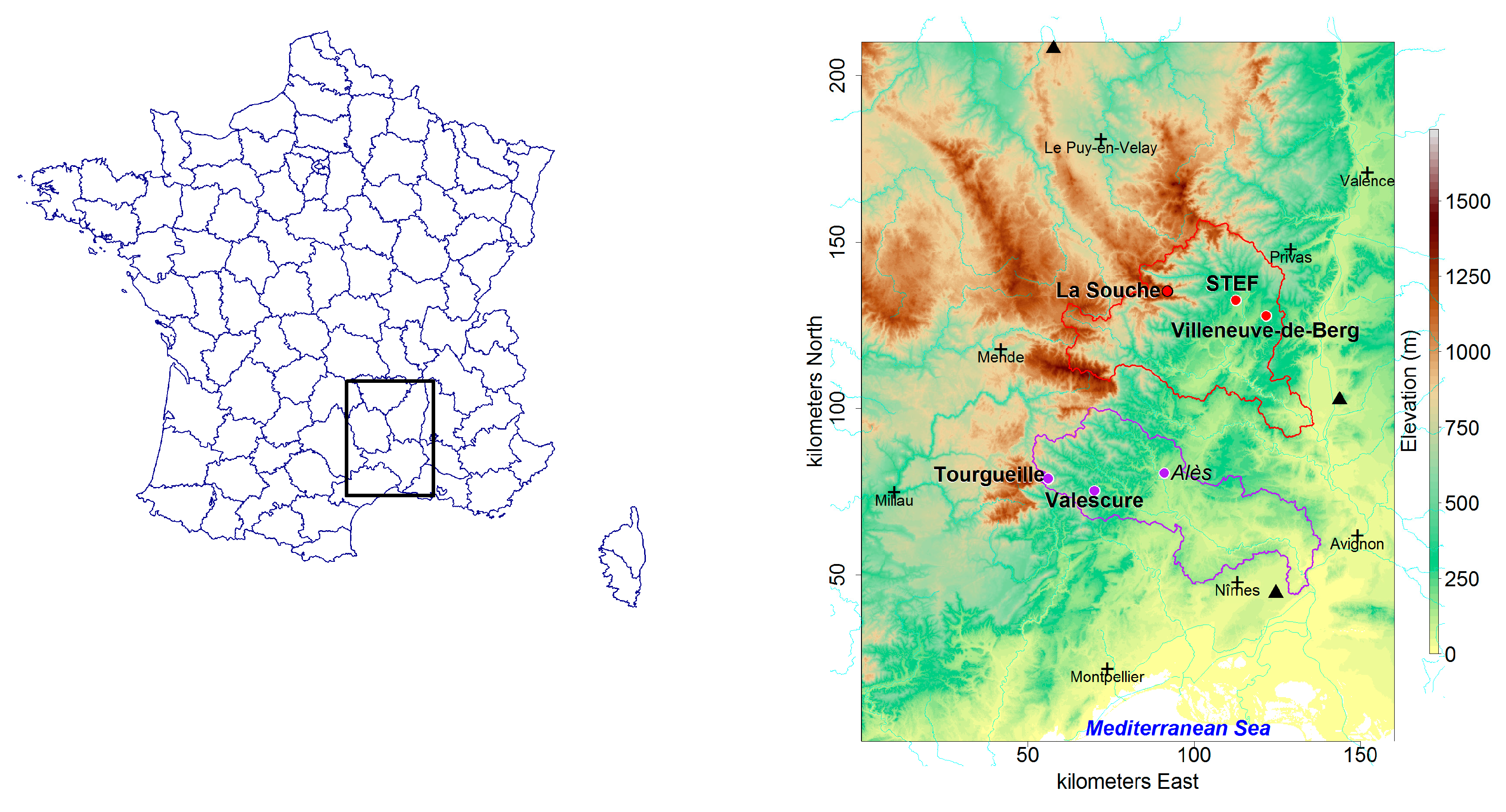
The data used for this study comes from part of a network of optical disdrometers (Figure 1) distributed over the Cévennes-Vivarais region monitored by the OHMCV [14] national observation service. All the disdrometers in this network are of the same brand (OTT) and of the same type (Parsivel, [34]). However, two generations of this model have been installed over time; the oldest station is of the first generation (marked in italics on the map. It was shown that the second generation was an improvement over the first generation for both drop size and rainfall measurements [35]. This network was initiated in 2004 (Alès station, [30]) and was densified during the HyMeX project, whose special observation period (SOP) took place in 2012 [33]. During this SOP, the network contained up to 25 stations, half of which were grouped on a dense network called “Hpiconet” [36] and was centred on the Auzon watershed [37]. For this study, covering the period 2012–2016, six stations were selected, according to two transects, going from the mountain to a hilly area, via a transition zone at the foot of the first mountains. Their characteristics are reported in Table 1, in which altitudes are given for information. By “environment”, we mean the distance to the Cévennes Mountains.
2.2. Data Availability, Checking, Filtering and Correction
Data are available on the OHMCV [38] and HyMeX [39] databases in NetCDF format. The time step for data acquisition is one minute. Data were aggregated to five minutes, in order to ensure a sufficient amount of drops each time step. Only time steps for which the rainfall intensity was above 1 mm/h (considered to be enough intense for this climate) have been kept in this study.
Several DSD data filtering or correction methods were compared, by computing rainfall totals from DSD spectra and using as a reference, the daily totals of the available rain gauges closest to the disdrometers. The rain gauge corresponding to StEF’s disdrometer is located in Aubenas, at 2 km; the rain gauge corresponding to La Souche station is located 100 m from the disdrometer. All other rain gauges are located less than 5 m from the disdrometers. The daily time step was chosen, so as to limit the effects of the spatial and temporal variabilities of the rain, which may be strong in this region. Three filtering or correction methods were tested:
- The first method (S1) used the raw DSD spectra (number of drops in 32 × 32 size/fall speed classes each record) without any correction or filtering.
- The last one (S3) was the “correction” method, proposed by [42]. This method consisted of applying pre-determined correction factors, depending on the intensities and the diameters that were estimated during inter-comparison measurement campaigns, using a 2DVD (used as a reference) and Parsivels of both generations. These campaigns took place between September and November, in both 2012 and 2013, in the Cévennes-Vivarais region, and between April and June 2014 in Payerne (Switzerland) [42].
In addition, two more filters were applied to the S1, S2, and S3 methods, in order to exclude solid and mixed particles and/or data recorded when dirt was present on the protective glass of the laser disdrometer. This information about hydrometeor types and laser quality is given by the Parsivel itself.
The three processing methods, with or without application of the additional filters, were compared to the reference values, according to classical criteria (root mean square error, RMSE; determination coefficient; and relative error, RE) at daily time steps. The application of the two additional filters allowed us to slightly improve the scores and they were consequently used in the following tests. Time steps with snow and mixed precipitation were, therefore, discarded in the rest of the study. The worst scores were obtained with the raw data (R2 = 88.3%, RMSE = 5.93, RE = 31.3%). The “correction” method (S3) led to the best relative error (RE = –15.5% vs. 17.3%) while the “filtering” method (S2) allowed the best determination coefficient (R2 = 96.2% vs. 82.6%) and the best root mean square error (RMSE = 3.73 vs. 8.80) to be obtained. The “filtering” method (S2) was, therefore, been retained.
Some disdrometers had data gaps, due to problems with the motherboard of the device or power failures. Periods with dirty laser glass also caused gaps. However, after application of the filters, each disdrometer recorded at least more than 5600 five-minute rainy time steps during the five-year period, 2012–2016.
3. DSD Descriptors and External Factors Studied
3.1. DSD Descriptors
The DSD were described by the use of three variables:
(a) The characteristic diameter , defined by [43]:
with:
where (mmk m−3) is the kth moment of the DSD, is the drop diameter (mm), and is the DSD, expressed as the drop concentration per unit volume and unit diameter (m−3 mm−1).
(b) The variable , proposed by [43] represents a scaling parameter for the DSD concentration:
with:
where Γ is the gamma function.
(c) The shape parameter µ of the gamma probability distribution function, which is a distribution frequently used to model the DSDs [27,30,43]. µ can be expressed from the 2nd, 3rd, and 4th moments of the DSD [27]:
with:
The combination of these scaling parameters was chosen to characterise the drop concentration, characteristic diameter, and the DSD shape. Moments of orders, equal to or exceeding 2, were chosen to limit the effects of the truncation of the weakest diameters. Note that these three parameters are not statistically independent; N*, Dc and μ exhibit a rather small and negative correlation (correlation coefficients of −0.57 and −0.65, respectively), while that between N* and μ is somewhat higher and positive (0.72). It was shown in several studies (e.g., [27,30,43]) that fitting these three parameters allows us to obtain good modelling of instantaneous or averaged DSDs. The radar reflectivity factor Z (mm6 m−3) and the rainfall rate R (mm h−1) are derived from the 6th and the 3.67th moments of the observed DSDs, according to the following equations:
These equations assume the particular terminal velocity relationship proposed by [44].
The spatio-temporal variability of DSD parameters (N*, DC, µ) was analysed using box-and-whisker plots of their statistical distributions. The box-and-whisker plots were represented, either for each station separately (temporal variability), for all stations combined or for groups of stations, taking into account the influence of the location. An analysis of variance was systematically performed to check the statistical significance of the results.
The relationship between dBZ (10 × log10(Z)) and dBR (10 × log10(R)) will be represented in the following the first time as a scatterplot, and then with 80% confidence ellipses (normal-probability contours) of the scatterplots, in order to facilitate readability and to allow the observation of trends, according to the external factors presented in the next section.
3.2. External Factors Studied
The DSD parameters and the 80% confidence ellipses around the Z-R scatterplots were studied according to four external factors that potentially explain a part of spatial and/or temporal variability: (1) location in terms of proximity of the Mediterranean Sea (the south part of the region is located closer to the sea) and proximity of the mountain (the west part of the region is mountainous; the east part is composed of small hills); (2) season; (3) daily synoptic weather situation, and (4) rainfall type.
3.2.1. Location
In order to study the influence of the location, data from the measurement stations have been grouped in two ways:
- (1)
- According to the proximity of the sea: data from La Souche, STEF, and Villeneuve stations have been put together to represent the climate of the north of the area, furthest from the Mediterranean Sea; data from Tourgueille, Valescure, and Alès have been put together to represent the south part of the area, where the Mediterranean character of the climate is more pronounced.
- (2)
- According to the proximity of the Cévennes mountains: data from La Souche and Tourgueille, which are located near mountain passes have been put together and labelled as “mountain”; data from Villeneuve and Alès, which are located in hilly areas in the plains have been put together and labelled as “hills”. Finally, the two remaining stations—STEF and Valescure—located, respectively, in the Ardèche valley and near the St Jean’s Gardon valley, have been labelled as “transition”.
3.2.2. Season
The Mediterranean climate is well known for its rainfall seasonality [45]. In the Cévennes-Vivarais region, the highest rain totals occur during fall season and the weakest during summer [6,7]. In this study, we distinguished DSD and Z-R properties as a function of meteorological seasons (e.g., summer corresponds to June, July, and August; fall season corresponds to September, October, and November, etc.).
3.2.3. Daily Synoptic Weather Pattern (WP)
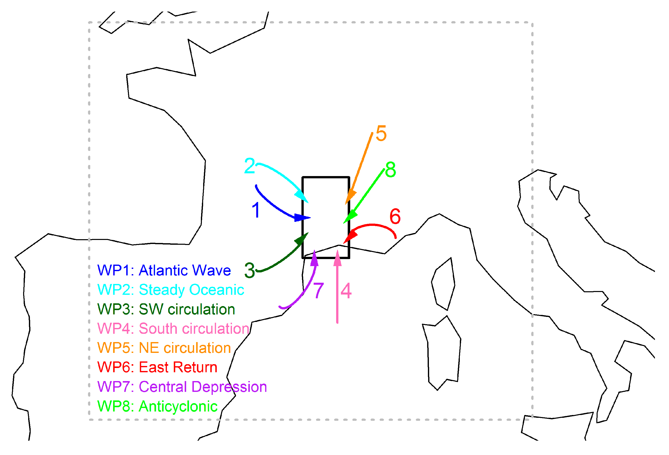
A daily weather classification [46] was provided by EDF/DTG (Electricité de France, Direction Technique Générale) for the studied period (2012–2016). It is derived from geopotential height fields, at 700 and 1000 hPa fields, at 00 h and 24 h, for the area delimited by the grey dashed rectangle in Figure 2. This classification contains eight contrasting synoptic situations for France. It was designed to explain the patterns of the rain fields in Southern France. Figure 2 summarizes the eight classes and the corresponding origins of the incoming atmospheric flow in the lower layers of the area of interest (the black rectangle corresponds to the Cévennes-Vivarais region plotted on Figure 1):
- WP1: Atlantic Wave (21% of rainy time steps)
- WP2: Steady Oceanic (10%)
- WP3: Southwest Circulation (7%)
- WP4: South Circulation (27%)
- WP5: Northeast Circulation (14%)
- WP6: East Return (4%)
- WP7: Central Depression (15%)
- WP8: Anticyclonic (2%)
In this region, WP4, 6, and 7 (“central depression” here means that the low is located on the near Atlantic and at the origin of the warm and moist Mediterranean airflow) bring the most important contributions to the inter-annual mean precipitation, whereas WT 2, 5, and 8 bring the less important totals. In the total of the 5-min rainy time steps recorded by the six disdrometers, WP1 and 4 are the most frequent: 48% of the rainy time steps occurred during one of those WPs. WP6 and 8 are the least frequent: 6% of the rainy time steps occur during one of those WPs.
3.2.4. Rainfall Type
Rainy time steps, corresponding to a selection of 55 rain events, during part of the study period (2012–2014), were classified according to six rainfall types:
- (1)
- Organized convective system (Org)
- (2)
- Isolated thunderstorms (Iso)
- (3)
- Showers (Sh)
- (4)
- Orographic rain (Oro)
- (5)
- Stratiform light rains (Str)
- (6)
- Scattered rain (Sca)
This classification was proposed based on the experience we have on precipitation in this area and was carried out from radar-based operational quantitative precipitation estimates from Météo-France [48] at five-minute step times and 1 km2 resolution. The rainfall type was empirically identified on each of the five-minute radar images for the overall area of interest. Only the rainy time steps with more than 1 mm h−1 during five-minute periods, in 2012–2014, for which the rainfall type was identified without ambiguity (no transition between or coexistence of several rainfall types) have been retained. The stratiform light rains (Str) represent 77% of the 12,707 analysed rainy time steps, while each of the other types occurs less than 6% of the time. Figure 3 illustrates a selection of six radar individual images, representing the 5-min rainfall totals, one for each rainfall type.
4. Results and Discussion
4.1. Location: Latitudinal and Longitudinal/Orographic Influences
Figure 4 shows, in the form of box-and-whisker plots, the distributions of the three DSD parameters for the stations of the Northern and Southern transects; the Z-R scatterplot, computed from the 5-min DSD data is displayed as well, together with the 80% confidence ellipses and the corresponding least-rectangles linear regression. Figure 4 shows that latitude had a small influence on DSD properties. Only the shape parameter was slightly higher in the south. This proves that the climate of this region is homogeneous, with respect to the distance to the sea. The median values of N*, Dc, and μ were, respectively, about 9000 drops m−3 mm−1, 1.1 mm, and 3. The dispersion was relatively large, with interquartile [Q1; Q3] values in the order of 10,000 drops m−3 mm−1 for concentration, 0.5 mm for characteristic diameter, and 5 for the shape parameter. The scatterplot between dBZ and dBR also exhibited a large dispersion. In such a case, as shown in [30], different fitting techniques may give significantly different Z-R relationships. The least-rectangle linear regression used herein is clearly not well suited for high rain-rate values. However, it was chosen because there was no reason to consider the rainfall rate or the reflectivity factor as the explanatory variable. Here, the aim was to obtain a qualitative assessment of the influence of the various factors considered, on the DSD parameters and the Z-R relationships coefficients.
Figure 5 represents the same kind of comparison for the longitude, which is associated, in this region, with different topographic environments. The orographic environment had a more visible influence on DSD parameters. By going from the mountain to the hills, all the N* quartiles decreased. Only the minimum value of N* was lower in the transition zone, making the dispersion of N* in this zone slightly greater. The two first quartiles of Dc increased, going from the mountain to the hills. The upper extremity of the Dc box-and-whisker plot had fairly similar values in the mountain and hills regions, but was higher in the transition zone where the dispersion was thus also greater. For the shape parameter, the quartiles 50%, 75%, and the upper extremity of the box-and-whisker plot decreased, going from the mountain to the hills. The increase of this parameter in the mountains may be explained by coalescence and break-up acting simultaneously [49].
The 80% confidence ellipses on the dBZ/dBR plot for mountainous and transition areas were close to each other and distinguishable from the plot for hilly areas. The ellipse for hills was shifted to larger values of Z, whatever the rain-rate range. This shift is consistent with the fact that the diameters are higher and the concentrations lower in the hills. This leads to higher reflectivity for equivalent rainfall rates. Note that the ellipse corresponding to the hills area was also slightly more flattened, as a result of the lower variability of the DSD parameters in this area. Note also that there would be fewer extreme values of rain-rate on the hills.
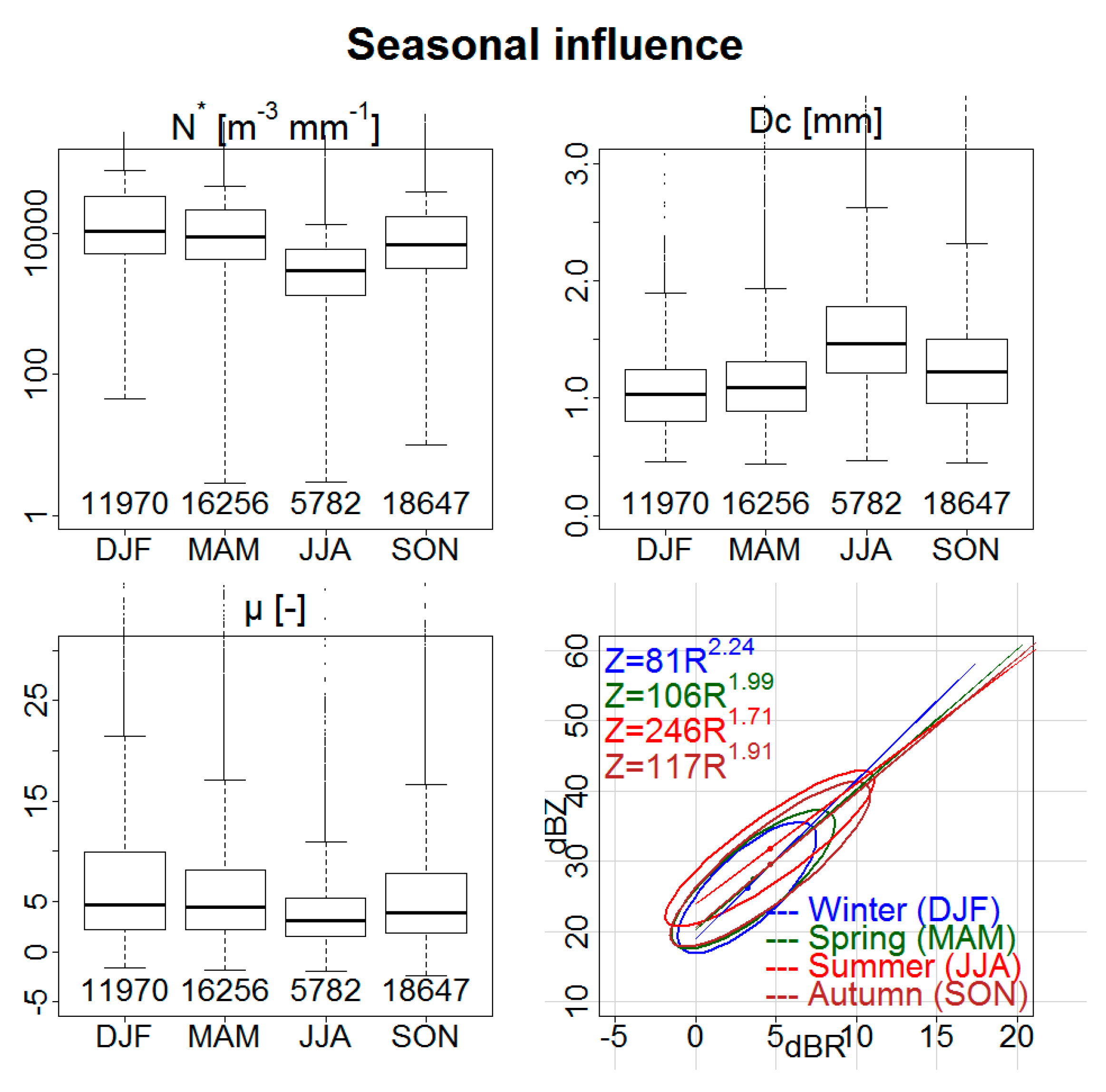
4.2. Seasonal Influence
Figure 6 represents, in the same manner, the influence of the seasons. Summer (JJA) was significantly different from the other seasons, with lower drop concentrations, higher characteristic diameters (the quartile Q1 of summer is equivalent to the quartile Q3 in winter), and with lower values and variability for µ. The Z-R relationship in summer differed from the other seasons, with a stronger pre-factor (corresponding to the intercept of the Z-R relationship in a log-log plot) and a lower exponent (with respect to the slope): for the same rain-rate (especially for weak to moderate rain-rates), the reflectivity factor was higher because of the larger diameters. This summer particularity can be explained by the greater number of convective rain events and this encourages the use of a Z-R relation adapted to this type of rain during summer.
The three other seasons have in common, the quartiles, Q1 and Q2, which are fairly close for all three parameters. The 80% confidence ellipses on the Z-R plot are superimposed for the low and medium intensities. However, we can distinguish some specificity on pairs of seasons that depend on the parameters:
- (1)
- Distributions of Dc were almost identical in winter and spring. During these seasons, the dispersion of values is the lowest;
- (2)
- Distributions of μ were almost identical in spring and autumn; and
- (3)
- The concentration of drops was most similar in autumn and winter, when they were also highest (especially in winter).
The seasonal cycles of the different parameters are, therefore, shifted in time: concentration is the first parameter that progress during the spring, with more dispersion towards smaller values; the dispersion of the shape parameter decreases. Then, during summer, the characteristic diameters increase significantly and remain relatively large during fall season. However, during fall season, the distribution of μ become the same as during spring and the distribution of concentrations is already much closer to that of winter.
In autumn, all parameters have intermediate characteristics between summer and winter. The 80% confidence ellipse of the Z-R plot during autumn was similar to those of winter and spring, for low and medium rainfall rates values, while it merged with that of summer for high rainfall rates. Spring was intermediate for μ and N*, but not for Dc, whose characteristics were closer to those of winter.
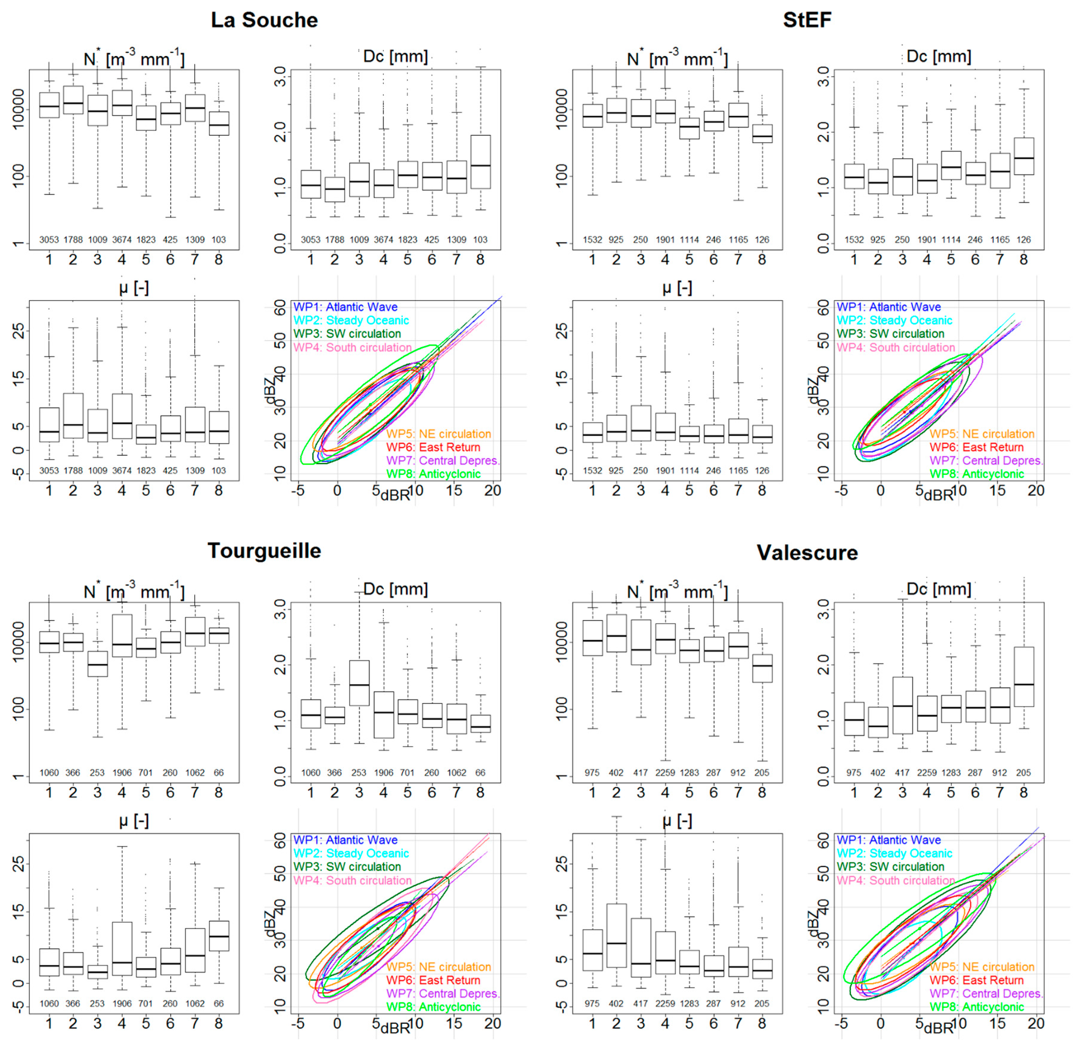
4.3. Daily Weather Pattern Influence
Figure 7 represents the influence of weather patterns (WP) on DSD characteristics and the Z-R relationship using the whole DSD dataset. Two groups can be identified:
- (1)
- WP3, 5, 6, and 8 are characterized by both lower concentrations, stronger characteristic diameters, and lower shape parameters;
- (2)
- WP1, 2, 4, and 7 that are characterized by higher concentrations, lower characteristic diameters (except for WP7 and slightly WP4 due to high dispersion) and more important shape parameters.
In these rather coarse groups, however, particular WPs stand out:
- WP8 (Anticyclonic) is the most particular of the first group, especially in terms of concentration (very low) and characteristic diameter (very large). This explains the shifted position towards the high Z values of the 80% confidence ellipse of this WP on Z-R plot. This type of weather, however, corresponds to weak occurrences of rain. The precipitating systems formed during this type of weather are generally small isolated thunderstorms.
- WP3 (Southwest Flow) brings more frequent precipitation to this region than WP8. It has similar, but less marked, characteristics.
- WP7 (Central Depression) brings high rainfall totals over the entire region. This is the only WP for which the concentration parameter is not anti-correlated with the characteristic diameter; drops are both numerous and large.
- WP5 (Northeast Circulation) corresponds to the smallest DSD variability. This WP brings very little precipitation over the region.
- Conversely, WP4 (South Circulation) is the one for which the DSD parameters are most variable. As it corresponds to a Southern flow in the lower layers, it favours incoming air masses from the sea and can trigger precipitation only on the first foothills of the reliefs.
The confidence ellipses on Z-R plots all have roughly the same large flattening; the underlying scatterplots thus remain much dispersed. They are also almost all aligned. This means that the Z-R relationship is not, at first sight, dependent on the WP. Only the ellipse corresponding to the rains occurring during anticyclonic WP is distinguished from the others, with the specificities seen previously for the summer season. Two other ellipses, corresponding to east and northeast flows, also have a peculiarity for low to medium rainfall rate values; the reflectivity factors are slightly higher. This is due to the fact that the Q1 for Dc is quite high and that of N* is fairly low.
4.4. Rainfall Type Influence
Figure 8 shows the influence of rainfall types in the same way as in the previous figures. It clearly highlights that the most discriminating factor is the rainfall type. It is observed that the values of the DSD parameters are very dependent on the degree of convection of the precipitating systems. The quartiles of the characteristic diameter (with respect to the shape and concentration parameters) decrease (with respect to the increase), moving from organized convective systems and isolated thunderstorms, to showers and stratiform rains. The dispersion of characteristic diameters is more important for rainfalls of convective types (Org, Iso, and Sh), while that of the shape parameter is more important for scattered rains and orographic rains. The orographic precipitations present the same properties as showers for characteristic diameter and the Z-R relationship and are close to those of scattered rainfalls for concentration and shape parameters.
The 80% confidence ellipses corresponding to the different rainfall types are particularly contrasting. This confirms that the rain type is one of the most discriminating factors in Z-R relationships. There are three different slopes (exponents of the Z-R relationship): (a) fairly high, common for stratiform, orographic rains and showers which correspond to low and medium rain-rates; (b) weaker, for isolated thunderstorms, for which rain-rates may be more extreme; and (c) even lower, for organized convective systems, that lead to the highest rain-rates. The intercept (pre-factor of the Z-R relation) of the major axis of the ellipses increases from scattered rains to organized convective systems. Convective rains have more flattened ellipses, indicating less dispersed Z-R relationships. This confirms that convective events generally tend to have smaller Z-R exponents in this area [31]. Finally, the orographic rains have a Z-R similar to those of the showers. Therefore, the interest in a convective-stratiform identification (as in [29]) for the precipitation quantitative estimation is confirmed. To a lesser extent, a distinction between the pre-factors, used for stratiform and orographic rains, also seems useful.
4.5. Combined Influences
The strong contrast found in DSD characteristics and Z-R relationships were not explained by the seasons (except for summer) or weather pattern (except for WP8). However, if the location is taken simultaneously into account, new contrasts do appear.
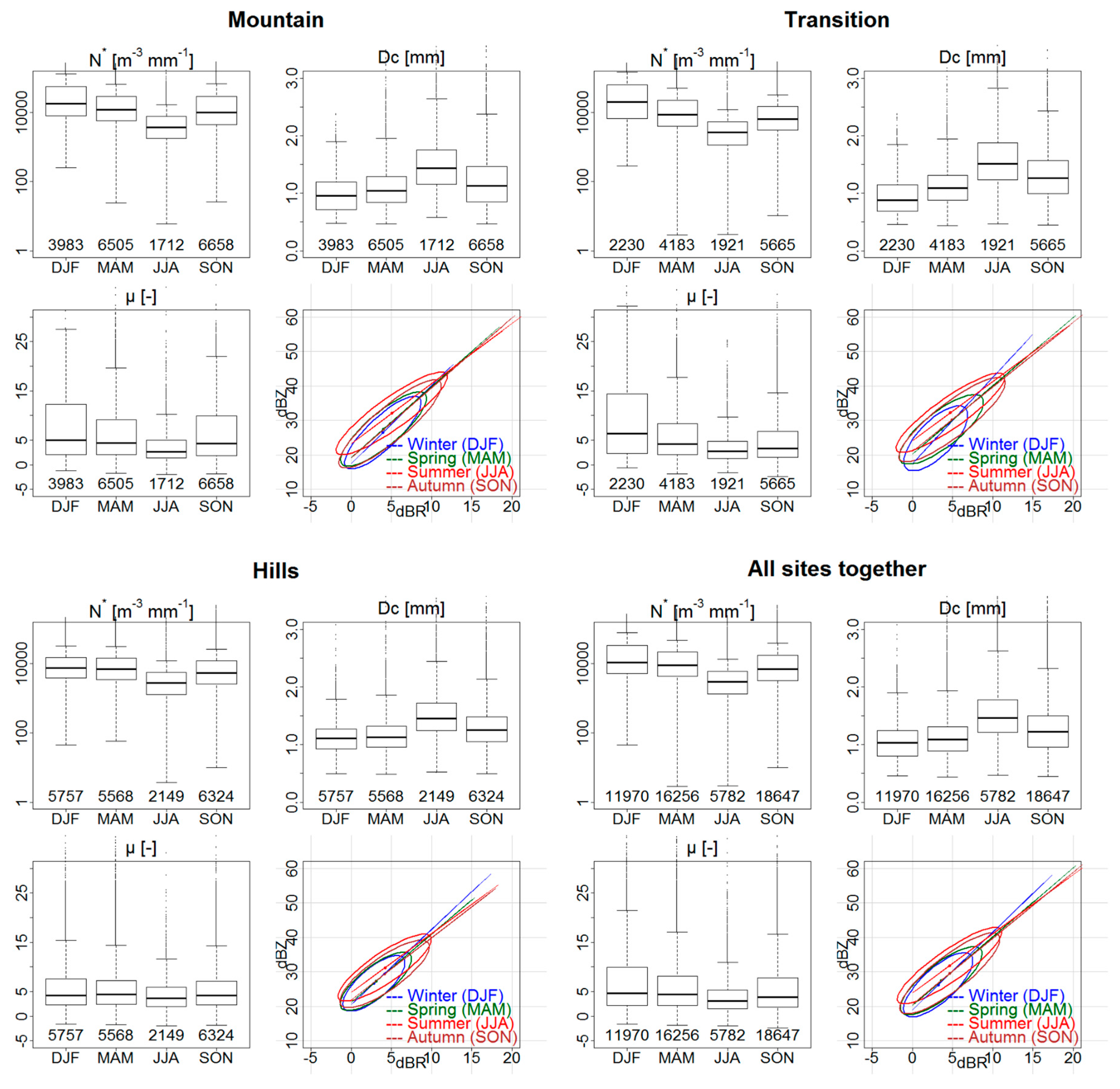
4.5.1. Seasons and Locations
Figure 9 is a composition of Figure 6 for each topographic environment. The evidence from this new presentation suggests that the shape parameter is less sensitive to the seasons in the hill area, but more sensitive in the mountainous and the transition areas. The trend to more variability existed also for Dc and N* but in a more discrete way. Concerning Z-R plots, the main findings for all of Cévennes-Vivarais remain valid for the hill and mountainous areas. However, the ellipses were organized in a different manner for transition areas in winter, with a steeper slope (bigger Z-R exponent), due to higher concentrations and lower diameters in this area during this season.
4.5.2. Weather Patterns and Locations
The same analysis was carried out on weather patterns, by seeking trends explained by latitude or longitude. For latitudes, no difference was found between north and south parts of the Cévennes-Vivarais region (not shown). For longitudes, only a few more important dispersions were found for the shape parameter during WP7 and WP8 in the mountains, and during WP3, 4, 7, and 8 in the transition area (not shown). However, no consequence was observed on Z-R plots. These results suggest that the distance from the sea or from the mountainous area, combined with weather patterns has no, or very little, influence on DSD characteristics and Z-R relationships.
However, strong variability appeared when the stations of the transition and mountain areas were separately analysed. Figure 10 is a composition of Figure 7 for the DSD stations located in these areas. It shows that the distributions of N* and Dc, according to weather patterns, were consistent between the two stations of the north. Those of Valescure were slightly more contrasting, especially during WP3, for which the Dc values are bigger and those of N* are more scattered. The distributions of N* and Dc for Tourgueille were totally different, again, especially for WP3, with very large drops and small concentrations. WP3 characteristics (discussed in Section 4.3) are, thus, exacerbated in the mountainous context. Concerning the distributions of the shape parameter, they were considerably different at each location depending on the weather patterns. The shape parameter appears to be very sensitive to local configuration; it seems that the high values and high variability of µ are related to the exposure of the site to the wind. Indeed, the site of Tourgueille, which is oriented southeastward, has a higher µ for Mediterranean fluxes (WP4 and 7), while the site of Valescure, which is oriented westward, has higher µ quartiles for oceanic fluxes (WP1, 2, and 3).
Concerning the Z-R relationships, the parameters were different, according to the sites. For La Souche’s station, the intercept and the pre-factors were not sensitive to weather patterns, except for Northeastern circulations, WP 5 and 6, for which the slope was slightly lower, and WP8, for which the intercept was slightly higher. This is related to the relatively high values of Dc and low values of N* for these WP at this place. At Valescure station, the intercept and the pre-factors were also not sensitive to weather patterns, except for WP8, for which the intercept was again higher. The reasons are the same. At StEF station, the slope was not sensitive to weather patterns, but the intercepts were different according to them. Finally, at Tourgueille station, both intercepts and slopes were sensitive to weather patterns. Here, WP3 had the same behaviour as WP8 at the other stations, due to the large drops and small concentrations mentioned in the previous paragraphs. At this station, oriented toward Mediterranean fluxes, the Z-R slope is steeper for these circulations.
5. Conclusions
The DSD climatology that was established over five years on the Cévennes-Vivarais region from six OTT Parsivel optical disdrometers, distributed along two longitudinal transects, confirmed and/or showed that:
- (1)
- The distance from the Mediterranean Sea has a weak influence on DSD in the area considered in this study.
- (2)
- The summer season has larger drops, lesser concentration, and weaker shape parameters. Consequently, the Z-R relationship is quite different in this season, with a clear convective footprint (lower exponent and higher pre-factor).
- (3)
- The spring and fall season are transition seasons with hybrid characteristics between those of winter and summer. However, it was observed that there were differences between transition periods, according to DSD parameter: N* changes as early as spring, whereas Dc changes later in the summer season.
- (4)
- The weather patterns distinguish themselves in DSD characteristics and the Z-R relationship, but the differences are exacerbated in mountainous and transition areas, where the exposure of the site to atmospheric flow in the lower atmospheric layers particularly influences the shape parameter. The differences are attenuated in low altitude hilly areas.
- (5)
- The orographic environment also influences the size and concentration, depending on whether the site is located inside, close to, or far from mountainous areas, as found on one case study in [31].
- (6)
- The rainfall type strongly influences DSD characteristics and Z-R relationships. The convective rainfalls are particularly different than those usually found in the literature. This study proposes to detail a few more rainfall types, distinguishing six categories. A noteworthy gradation was found in the concentration, size, and shape parameters, according to the level of convection and organisation. Otherwise, the orographic precipitations present similar properties as showers for the characteristic diameter and the Z-R relationship. They are close to those of scattered rainfalls for concentration and shape parameter.
This study analysed mainly the trends on the relationship coefficients for each external factor. A study will be led on the same dataset to obtain Z-R relationships, suited for radar data processing, as well as to assess errors in quantitative precipitation estimates, due to DSD variability, according to the same external factors, on a large and medium scale, independently of other radar sources of errors (calibration, VPR, sampling issues). The future study will also illustrate the large amount of spatial and temporal variability that remains within the precipitation systems. Finally, another study is expected to extend this climatology to other Mediterranean locations (South Alps, Corsica, Spain, Italy, and Tunisia) in the framework of the HyMeX project.
Acknowledgments
The authors thank the providers of operational data: Météo-France for rain gauge data and radar data, and EDF for weather patterns. They warmly thank the colleagues of IGE’s technical staff who helped in installing and maintaining the observation system over several years: Romain Biron, Martin Calianno, Simon Gérard, Matthieu Le Gall, Coralie Aubert, Jean-Paul Laurent, Catherine Coulaud, Hélène Guyard, Frederic Cazenave, and Stéphane Boubkraoui. In addition, the authors acknowledge people who hosted the experiments: Jean Mazel (La Souche), the municipality of Saint-Etienne-de-Fontbellon (StEF), the secondary school (collège) of Villeneuve-de-Berg, Pierre-Alain Ayral and Rosario Spinelli at Ecole des Mines d’Alès, as well as Jean-François Didon-Lescot, Jean-Marc Domergue, and Nadine Grard at UMR ESPACE for their valuable contribution for the maintenance of the disdrometers of Tourgueille and Valescure. The authors acknowledge Hervé Andrieu (IFSTTAR) and Victor Le Boulch (ENTPE) for their valuable contribution to rainfall typing. Disdrometers were funded by OHMCV, ANR FloodScale, HyMeX, and Région Rhône-Alpes. The publication costs were covered by HyMeX. OHMCV is supported by the “Institut National des Sciences de l’Univers” (INSU/CNRS), the French Ministry for Education and Research, the “Observatoire des Sciences de l’Univers de Grenoble” (OSUG), and the “SOERE Réseau des Bassins Versants” (Alliance Allenvi). The FloodScale project is funded by the French National Research Agency (ANR) under contract no. ANR 2011 BS56 027, which contributes to the MISTRALS/HyMeX programme (http://www.mistrals-home.org). IGE is part of Labex OSUG@2020 (ANR10 LABX56), which funded the contract of Martin Calianno. The HyMeX database teams (ESPRI/IPSL and SEDOO/Observatoire Midi-Pyrénées) and the team of the OSUG data centre helped in accessing the data and attributing DOIs to the individual datasets. Sahar Hachani’s thesis was funded by IRD and Université Tunis El Manar.
Author Contributions
Brice Boudevillain conceived and designed the experiments and performed the experiments with the support of the IGE’s technical staff. Sahar Hachani (PhD student) and Brice Boudevillain (PhD advisor) analysed the data, contributed materials/analysis tools and wrote the paper. Zoubeida Bargaoui and Guy Delrieu provided advice and an internal review of the article.
Conflicts of Interest
The authors declare no conflict of interest. The founding sponsors had no role in the design of the study; in the collection, analyses, or interpretation of data; in the writing of the manuscript; or in the decision to publish the results.
References
- Frei, C.; Schär, C. A precipitation climatology of the Alps from high-resolution rain-gauge observations. Int. J. Climatol. 1998, 18, 873–900. [Google Scholar] [CrossRef]
- Tarolli, P.; Borga, M.; Morin, E.; Delrieu, G. Analysis of flash flood regimes in the North-Western and South-Eastern Mediterranean regions. Nat. Hazards Earth Syst. Sci. 2012, 12, 1255–1265. [Google Scholar] [CrossRef] [Green Version]
- Thiébault, S.; Moatti, J.P. (Eds.) The Mediterranean Region under Climate Change: A Scientific Update; AllEnvi: Marseille, France, 2016. [Google Scholar]
- Météo-France. Pluies extrêmes en France Métropolitaine. Available online: http://pluiesextremes.meteo.fr/ (accessed on 24 September 2017).
- Nuissier, O.; Ducrocq, V.; Ricard, D.; Lebeaupin, C.; Anquetin, S. A numerical study of three catastrophic precipitating events over southern France. I: Numerical framework and synoptic ingredients. Q.J.R. Meteorol. Soc. 2008, 134, 111–130. [Google Scholar] [CrossRef]
- Molinié, G.; Ceresetti, D.; Anquetin, S.; Creutin, J.D.; Boudevillain, B. Rainfall Regime of a Mountainous Mediterranean Region: Statistical Analysis at Short Time Steps. J. Appl. Meteorol. Climatol. 2012, 51, 429–448. [Google Scholar] [CrossRef]
- Froidurot, S.; Molinié, G.; Diedhiou, A. Climatology of observed rainfall in Southeast France at the Regional Climate Model Scales. Clim. Dyn. 2016, 1–19. [Google Scholar] [CrossRef]
- Ceresetti, D.; Molinié, G.; Creutin, J.D. Scaling properties of heavy rainfall at short duration: A regional analysis. Water Resour. Res. 2010, 46. [Google Scholar] [CrossRef]
- Miniscloux, F.; Creutin, J.D.; Anquetin, S. Geostatistical Analysis of Orographic Rainbands. J. Appl. Meteorol. 2001, 40, 1835–1854. [Google Scholar] [CrossRef]
- Berne, A.; Delrieu, G.; Boudevillain, B. Variability of the spatial structure of intense Mediterranean precipitation. Adv. Water Resour. 2009, 32, 1031–1042. [Google Scholar] [CrossRef]
- Ricard, D. Initialisation et Assimilation de Données à Méso-échelle Pour la Prévision à Haute Résolution des Pluies Intenses de la Région Cévennes-Vivarais. Ph.D. Thesis, Université Paul Sabatier-Toulouse III, Toulouse, France, December 2002. [Google Scholar]
- Godart, A.; Anquetin, S.; Leblois, E.; Creutin, J.D. The Contribution of Orographically Driven Banded Precipitation to the Rainfall Climatology of a Mediterranean Region. J. Appl. Meteorol. Climatol. 2011, 50, 2235–2246. [Google Scholar] [CrossRef]
- Marchi, L.; Borga, M.; Preciso, E.; Gaume, E. Characterisation of selected extreme flash floods in Europe and implications for flood risk management. J. Hydrol. 2010, 394, 118–133. [Google Scholar] [CrossRef]
- Boudevillain, B.; Delrieu, G.; Galabertier, B.; Bonnifait, L.; Bouilloud, L.; Kirstetter, P.E.; Mosini, M.L. The Cévennes-Vivarais Mediterranean Hydrometeorological Observatory database. Water Resour. Res. 2011, 47. [Google Scholar] [CrossRef]
- Delrieu, G.; Boudevillain, B.; Nicol, J.; Chapon, B.; Kirstetter, P.E.; Andrieu, H.; Faure, D. Bollène-2002 Experiment: Radar Quantitative Precipitation Estimation in the Cévennes-Vivarais Region, France. J. Appl. Meteorol. Climatol. 2009, 48, 1422–1447. [Google Scholar] [CrossRef]
- Zawadzki, I. Factors affecting the precision of radar measurements of rain. In Proceedings of the 22nd Conference on Radar Meteorology, Zurich, Switzerland, 10–13 September 1984; pp. 251–256. [Google Scholar]
- Chen, Y.; Takara, K.; Cluckie, I.D.; De Smedt, F.H. (Eds.) GIS and Remote Sensing in Hydrology, Water Resources and Environment; IAHS Publication: Wallingford, UK, 2004. [Google Scholar]
- Uijlenhoet, R. Raindrop size distributions and radar reflectivity-rain rate relationships for radar hydrology. Hydrol. Earth Syst. Sci. 2001, 5, 615–627. [Google Scholar] [CrossRef]
- Cerda, A. Rainfall drop size distribution in the Western Mediterranean basin, Valencia, Spain. CATENA 1997, 30, 169–182. [Google Scholar] [CrossRef]
- Yu, N.; Boudevillain, B.; Delrieu, G.; Uijlenhoet, R. Estimation of rain kinetic energy from radar reflectivity and/or rain rate based on a scaling formulation of the raindrop size distribution. Water Resour. Res. 2012, 48. [Google Scholar] [CrossRef]
- Angulo-Martínez, M.; Beguería, S.; Kyselý, J. Use of disdrometer data to evaluate the relationship of rainfall kinetic energy and intensity (KE-I). Sci. Total Environ. 2016, 568, 83–94. [Google Scholar] [CrossRef] [PubMed]
- Carollo, F.G.; Ferro, V.; Serio, M.A. Estimating rainfall erosivity by aggregated drop size distributions. Hydrol. Process. 2016, 30, 2119–2128. [Google Scholar] [CrossRef]
- Delrieu, G.; Creutin, J.D.; Saint-Andre, I. Mean KR Relationships: Practical Results for Typical Weather Radar Wavelengths. J. Atmos. Ocean. Technol. 1991, 8, 467–476. [Google Scholar] [CrossRef]
- Anagnostou, M.N.; Kalogiros, J.; Anagnostou, E.N.; Tarolli, M.; Papadopoulos, A.; Borga, M. Performance evaluation of high-resolution rainfall estimation by X-band dual-polarization radar for flash flood applications in mountainous basins. J. Hydrol. 2010, 394, 4–16. [Google Scholar] [CrossRef]
- Sempere-Torres, D.; Porrà, J.M.; Creutin, J.D. A General Formulation for Raindrop Size Distribution. J. Appl. Meteorol. 1994, 33, 1494–1502. [Google Scholar] [CrossRef]
- Cerro, C.; Codina, B.; Bech, J.; Lorente, J. Modeling Raindrop Size Distribution and Z(R) Relations in the Western Mediterranean Area. J. Appl. Meteorol. 1997, 36, 1470–1479. [Google Scholar] [CrossRef]
- Yu, N.; Delrieu, G.; Boudevillain, B.; Hazenberg, P.; Uijlenhoet, R. Unified formulation of single-and multimoment normalizations of the raindrop size distribution based on the gamma probability density function. J. Appl. Meteorol. Climatol. 2014, 53, 166–179. [Google Scholar] [CrossRef]
- Caracciolo, C.; Porcu, F.; Prodi, F. Precipitation classification at mid-latitudes in terms of drop size distribution parameters. Adv. Geosci. 2008, 16, 11–17. [Google Scholar] [CrossRef]
- Sempere-Torres, D.; Sanchez-Diezma, R.; Zawadzki, I.; Creutin, J.D. Identification of stratiform and convective areas using radar data with application to the improvement of DSD analysis and Z-R relations. Phys. Chem. Earth 2000, 25, 985–990. [Google Scholar] [CrossRef]
- Chapon, B.; Delrieu, G.; Gosset, M.; Boudevillain, B. Variability of rain drop size distribution and its effect on the Z-R relationship: A case study for intense Mediterranean rainfall. Atmos. Res. 2008, 87, 52–65. [Google Scholar] [CrossRef]
- Hazenberg, P.; Yu, N.; Boudevillain, B.; Delrieu, G.; Uijlenhoet, R. Scaling of raindrop size distributions and classification of radar reflectivity–rain rate relations in intense Mediterranean precipitation. J. Hydrol. 2011, 402, 179–192. [Google Scholar] [CrossRef]
- Zwiebel, J.; Van Baelen, J.; Anquetin, S.; Pointin, Y.; Boudevillain, B. Impacts of orography and rain intensity on rainfall structure. The case of the HyMeX IOP7a event. Q. J. R. Meteorol. Soc. 2016, 142, 310–319. [Google Scholar] [CrossRef]
- Ducrocq, V.; Braud, I.; Davolio, S.; Ferretti, R.; Flamant, C.; Jansa, A.; Kalthoff, N.; Richard, E.; Taupier-Letage, I.; Ayral, P.A.; et al. HyMeX-SOP1: The field campaign dedicated to heavy precipitation and flash flooding in the Northwestern Mediterranean. Bull. Am. Meteorol. Soc. 2014, 95, 1083–1100. [Google Scholar] [CrossRef]
- Löffler-Mang, M.; Joss, J. An Optical Disdrometer for Measuring Size and Velocity of Hydrometeors. J. Atmos. Oceanic Technol. 2000, 17, 130–139. [Google Scholar] [CrossRef]
- Tokay, A.; Wolff, D.B.; Petersen, W.A. Evaluation of the New Version of the Laser-Optical Disdrometer, OTT Parsivel2. J. Atmos. Ocean. Technol. 2014, 31, 1276–1288. [Google Scholar] [CrossRef]
- Bousquet, O.; Berne, A.; Delanoe, J.; Dufournet, Y.; Gourley, J.; Van-Baelen, J.; Augros, C.; Besson, L.; Boudevillain, B.; Caumont, O.; et al. Multifrequency Radar Observations Collected in Southern France during HyMeX-SOP1. Bull. Am. Meteorol. Soc. 2015, 96, 267–282. [Google Scholar] [CrossRef] [Green Version]
- Nord, G.; Boudevillain, B.; Berne, A.; Branger, F.; Braud, I.; Dramais, G.; Gérard, S.; Le Coz, J.; Legoût, C.; Molinié, G.; et al. A high space-time resolution dataset linking meteorological forcing and hydro-sedimentary response in a mesoscale Mediterranean catchment (Auzon) of the Ardèche region, France. Earth Syst. Sci. Data 2017, 9, 221–249. [Google Scholar] [CrossRef]
- Observatoire Hydrométéorologique Méditerranéen Cévennes-Vivarais. Available online: http://www.ohmcv.fr/ (accessed on 5 November 2017).
- Hydrological Cycle in Mediterranean Experiment. Available online: http://www.hymex.org/ (accessed on 5 November 2017).
- Jaffrain, J.; Studzinski, A.; Berne, A. A network of disdrometers to quantify the small-scale variability of the raindrop size distribution. Water Resour. Res. 2011, 47. [Google Scholar] [CrossRef]
- Beard, K.V. Terminal Velocity Adjustment for Cloud and Precipitation Drops Aloft. J. Atmos. Sci. 1977, 34, 1293–1298. [Google Scholar] [CrossRef]
- Raupach, T.H.; Berne, A. Correction of raindrop size distributions measured by Parsivel disdrometers, using a two-dimensional video disdrometer as a reference. Atmos. Meas. Tech. 2015, 8, 343–365. [Google Scholar] [CrossRef]
- Testud, J.; Oury, S.; Black, R.A.; Amayenc, P.; Dou, X. The Concept of “Normalized” Distribution to Describe Raindrop Spectra: A Tool for Cloud Physics and Cloud Remote Sensing. J. Appl. Meteorol. 2002, 40, 1118–1140. [Google Scholar] [CrossRef]
- Atlas, D.; Srivastava, R.; Sekhon, R.S. Doppler radar characteristics of precipitation at vertical incidence. Rev. Geophys. 1973, 11, 1–35. [Google Scholar] [CrossRef]
- Bolle, H.J. (Ed.) Mediterranean Climate: Variability and Trends; Springer: Berlin, Germany, 2002. [Google Scholar]
- Garavaglia, F.; Gailhard, J.; Paquet, E.; Lang, M.; Garçon, R.; Bernardara, P. Introducing a rainfall compound distribution model based on weather patterns sub-sampling. Hydrol. Earth Syst. Sci. 2010, 14, 951–964. [Google Scholar] [CrossRef] [Green Version]
- Froidurot, S. Approche Multi-échelle Pourl’évaluation de la Pluie dans les Modèles Climatiques Régionaux. Étude dans le Sud-est de la France. Ph.D. Thesis, Université Grenoble Alpes, Grenoble, France, November 2015. [Google Scholar]
- Figueras i Ventura, J.; Tabary, P. The New French Operational Polarimetric Radar Rainfall Rate Product. J. Appl. Meteorol. Climatol. 2013, 52, 1817–1835. [Google Scholar] [CrossRef]
- Rosenfeld, D.; Ulbrich, C.W. Cloud microphysical properties, processes, and rainfall estimation opportunities. In Radar and Atmospheric Science: A Collection of Essays in Honor of David Atlas; Wakimoto, R.M., Srivastava, R., Eds.; American Meteorological Society: Boston, MA, USA, 2003. [Google Scholar]
Figure 1.
Cévennes-Vivarais region. The crosses indicate the main cities. The dots represent the OTT Parsivel disdrometers considered in this study. The triangles indicate the location of the radars.
Figure 1.
Cévennes-Vivarais region. The crosses indicate the main cities. The dots represent the OTT Parsivel disdrometers considered in this study. The triangles indicate the location of the radars.

Figure 2.
Atmospheric flows in the low atmospheric layers corresponding to weather patterns (WP) analysed on the grey dash rectangle according to the classification proposed by [46]. The arrows indicate atmospheric flows for the studied area represented by a black rectangle. Adapted from [46,47].

Figure 3.
Illustration of the six rainfall time steps at different types: each picture represents 5-min rainfall accumulation (mm/5’). The time steps chosen (in UTC) are: (a) 20/07/2014 8:05–8:10, (b) 21/05/2014 12:50–12:55, (c) 09/10/2014 01:00–01:05, (d) 04/11/2014 00:40–00:45, (e) 07/07/2014 10:10–10:15, and (f) 07/07/2014 14:40–14:45. The triangles indicate the location of the radars.
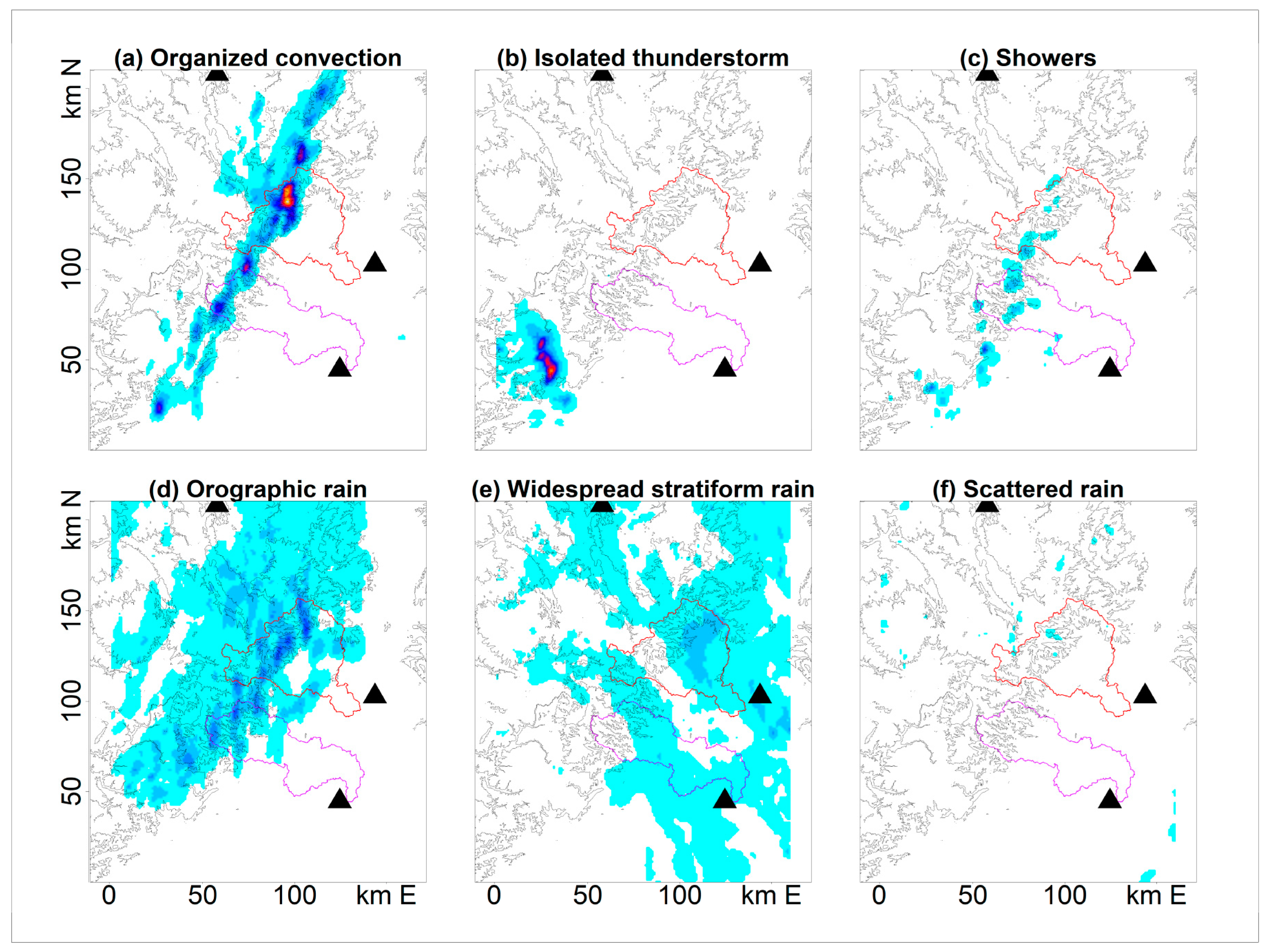
Figure 4.
Influence of latitude on DSD parameters: (a) scaling parameter for the DSD concentration; (b) characteristic diameter; (c) shape parameter; and (d) Z-R relationship. As usual, the boxes represent the quartiles, Q1, Q2, and Q3 (the quantiles 25%, 50%, and 75%, respectively). The lower whisker corresponds to the minimum value and the upper whisker corresponds here to Q3 + 1.5(Q3 − Q1). Values greater than the upper whisker are represented as individual points.
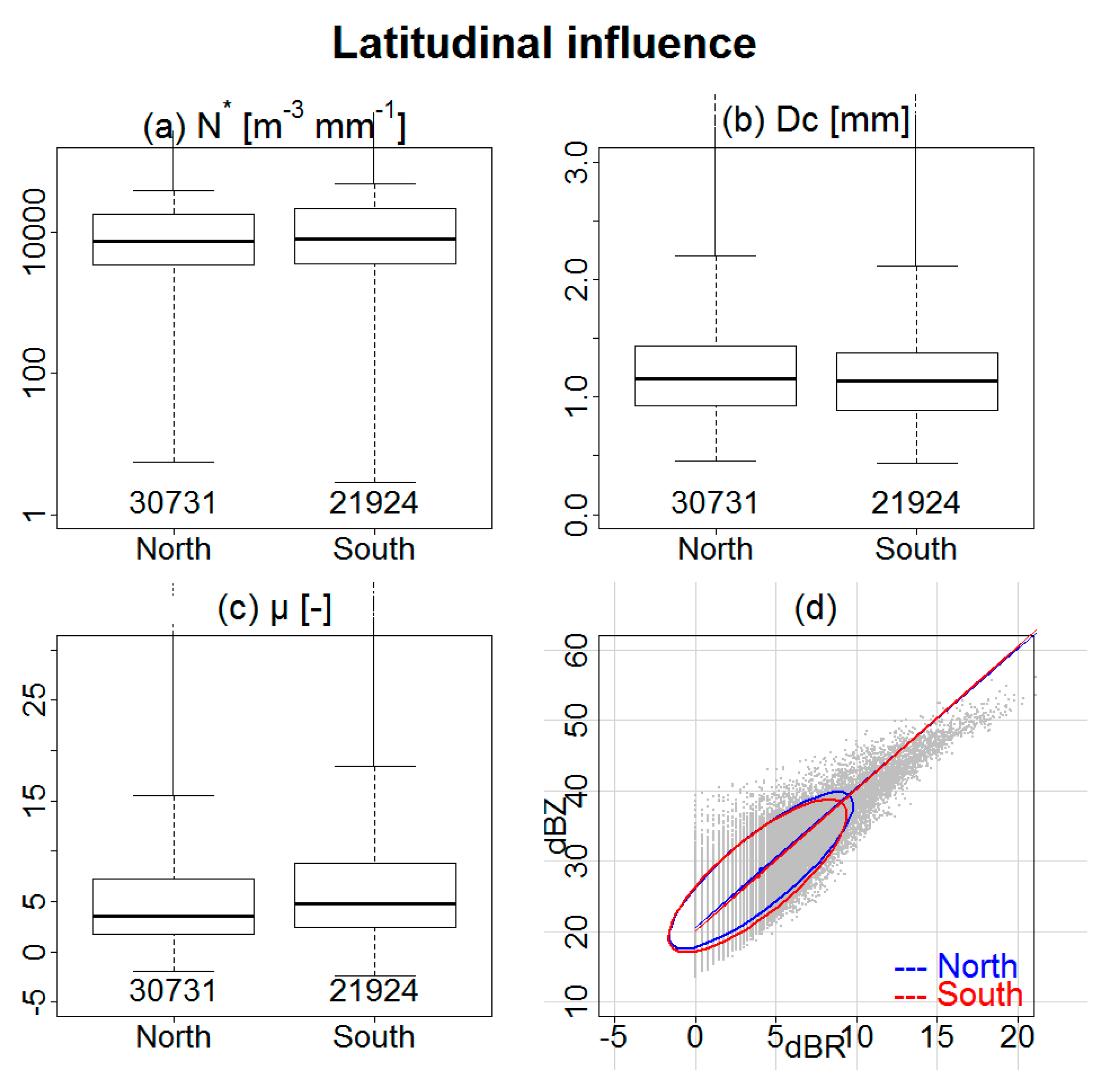
Figure 5.
Influence of a mountainous environment on DSD parameters and Z-R relationships.
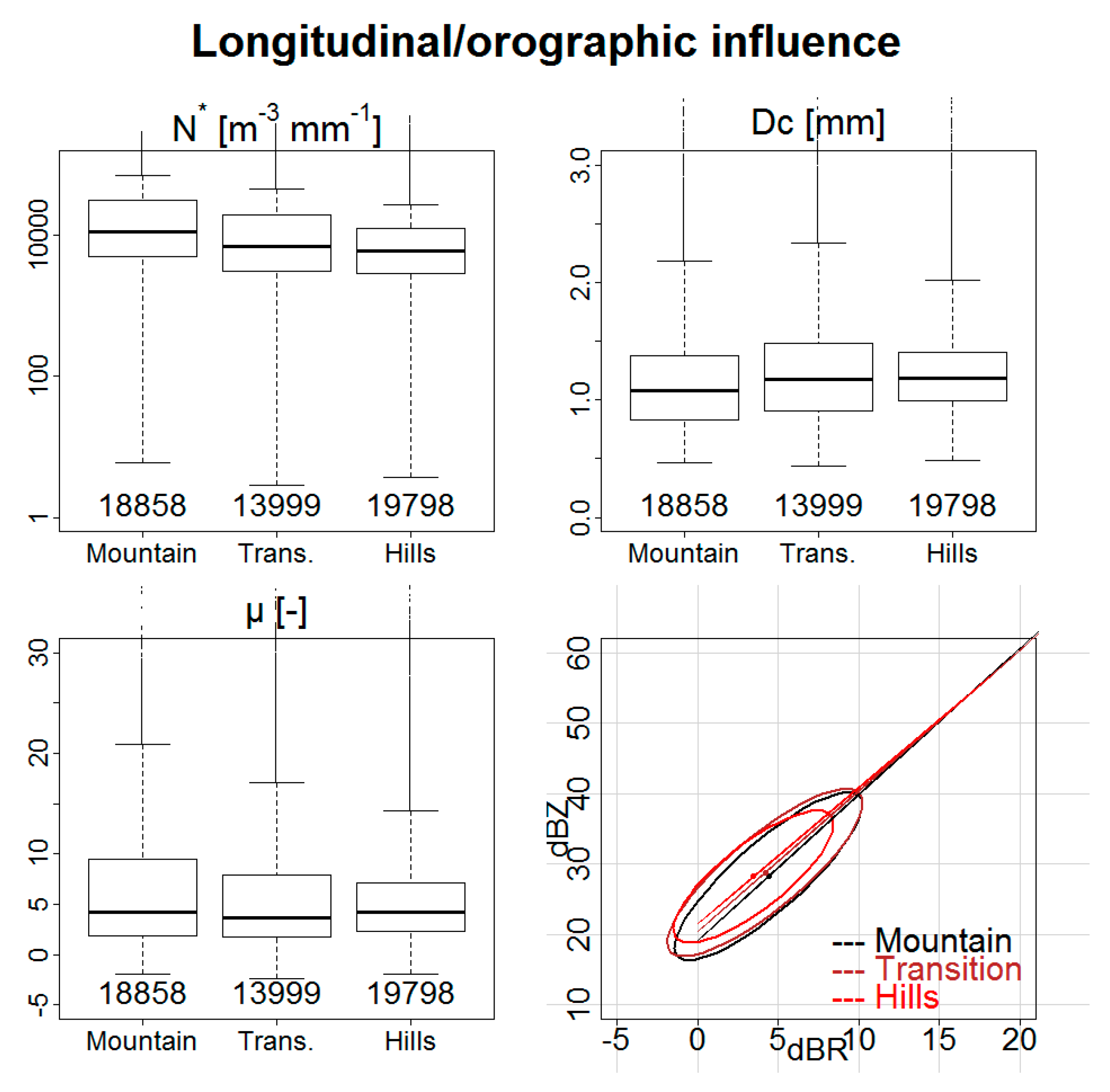
Figure 6.
Influence of seasons on DSD parameters and Z-R relationships.

Figure 7.
Influence of weather patterns on DSD parameters and Z-R relationships.

Figure 8.
Influence of rainfall types on DSD parameters and Z-R relationships.
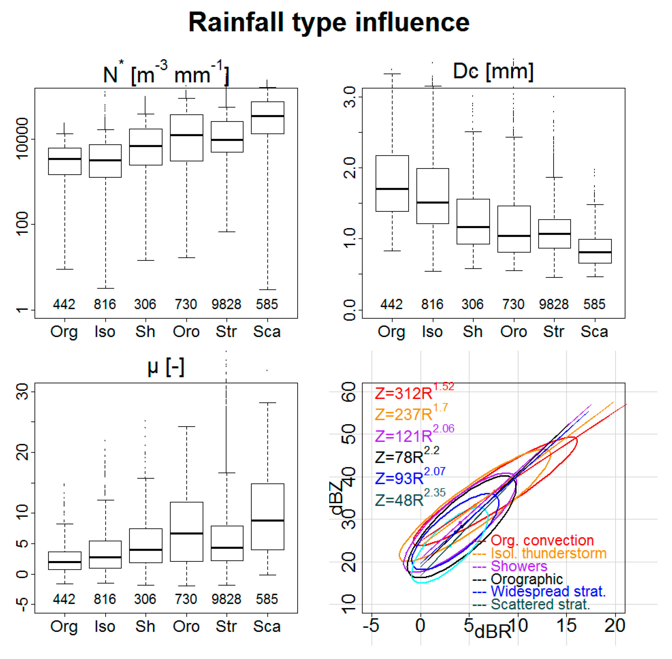
Figure 9.
Combined influences of seasons and locations.

Figure 10.
Combined influences of weather patterns and locations.


Table 1.
Location of the six disdrometer stations used in this study.
| ID 1 | Name | Location | Altitude | Disdrometer | Environment |
|---|---|---|---|---|---|
| SOU | La Souche | 44.63° N; 4.12° E | 920 m | OTT Parsivel2 | mountains |
| SEF | StEF | 44.60° N; 4.38° E | 210 m | OTT Parsivel2 | transition |
| VB1 | Villeneuve | 44.55° N; 4.50° E | 300 m | OTT Parsivel2 | hills |
| TOU | Tourgueille | 44.13° N; 3.66° E | 540 m | OTT Parsivel2 | mountains |
| VAL | Valescure | 44.09° N; 3.84° E | 480 m | OTT Parsivel2 | transition |
| ALE | Alès | 44.14° N; 4.10° E | 150 m | OTT Parsivel | hills |
1 DOIs of drop size distribution (DSD) datasets are named in following manner: 10.17178/OHMCV.DSD.XXX.12-16.1 where XXX is the ID given in the first row of the table.
© 2017 by the authors. Licensee MDPI, Basel, Switzerland. This article is an open access article distributed under the terms and conditions of the Creative Commons Attribution (CC BY) license (http://creativecommons.org/licenses/by/4.0/).
Share and Cite
MDPI and ACS Style
Hachani, S.; Boudevillain, B.; Delrieu, G.; Bargaoui, Z. Drop Size Distribution Climatology in Cévennes-Vivarais Region, France. Atmosphere 2017, 8, 233. https://doi.org/10.3390/atmos8120233
AMA Style
Hachani S, Boudevillain B, Delrieu G, Bargaoui Z. Drop Size Distribution Climatology in Cévennes-Vivarais Region, France. Atmosphere. 2017; 8(12):233. https://doi.org/10.3390/atmos8120233
Chicago/Turabian StyleHachani, Sahar, Brice Boudevillain, Guy Delrieu, and Zoubeida Bargaoui. 2017. "Drop Size Distribution Climatology in Cévennes-Vivarais Region, France" Atmosphere 8, no. 12: 233. https://doi.org/10.3390/atmos8120233
Note that from the first issue of 2016, this journal uses article numbers instead of page numbers. See further details here.