Evaluation of Surface Fluxes in the WRF Model: Case Study for Farmland in Rolling Terrain

1
Atmospheric Sciences Program, Department of Physics, University of Nevada, Reno, NV 89557, USA
2
Hebei Meteorology Bureau, Shijiazhuang 050021, China
*
Author to whom correspondence should be addressed.
Atmosphere 2017, 8(10), 197; https://doi.org/10.3390/atmos8100197
Submission received: 11 July 2017
/
Revised: 27 September 2017
/
Accepted: 2 October 2017
/
Published: 8 October 2017
(This article belongs to the Special Issue Atmospheric Processes over Complex Terrain)
Abstract
:The partitioning of available energy into surface sensible and latent heat fluxes impacts the accuracy of simulated near surface temperature and humidity in numerical weather prediction models. This case study evaluates the performance of the Weather Research and Forecasting (WRF) model on the simulation of surface heat fluxes using field observations collected from a surface flux tower in Oregon, USA. Further, WRF-modeled heat flux sensitivities to North American Mesoscale (NAM) and North American Regional Reanalysis (NARR) large-scale input forcing datasets; U.S. Geological Survey (USGS) and the Moderate Resolution Imaging Spectroradiometer (MODIS) land use datasets; Pleim-Xiu (PX) and Noah land surface models (LSM); Yonsei University (YSU) and Mellor-Yamada-Janjic (MYJ) planetary boundary layer (PBL) schemes using the Noah LSM; and Asymmetric Convective Model version 2 (ACM2) PBL scheme using PX LSM are investigated. The errors for simulating 2-m temperature, 2-m humidity, and 10-m wind speed were reduced on average when using NAM compared with NARR. Simulated friction velocity had a positive bias on average, with the YSU PBL scheme producing the largest overestimation in the innermost domain (0.5 km horizontal grid resolution). The simulated surface sensible heat flux had a similar temporal behavior as the observations but with a larger magnitude. The PX LSM produced lower and more reliable sensible heat fluxes compared with the Noah LSM. However, Noah latent heat fluxes were improved with a lower RMSE compared to PX, when NARR forcing data was used. Overall, these results suggest that there is not one WRF configuration that performs best for all the simulated variables (surface heat fluxes and meteorological variables) and situations (day and night).
1. Introduction
Surface fluxes serve as sinks or sources of energy, moisture, momentum, and atmospheric pollutants and significantly impact the formation and evolution of clouds, precipitation, and air pollution. Surface fluxes are crucial parameters for simulating convective mixing, boundary layer growth, and atmospheric transport [1]. The significance of land surface interactions with the atmosphere has been increasingly emphasized and investigated during numerical weather prediction (NWP) model (e.g., Weather Research and Forecasting (WRF) model) developments [2,3,4,5]. NWP models are subject to uncertainties in surface interaction parameterization, and parameter choice has significant effects on NWP outputs. For example, land surface model (LSM) selection was found to have large impacts on WRF simulation results during cold air pool events, since non-realistic representation of low-level jets could lead to errors in simulated temperature and humidity [6].
Reanalysis datasets, including the North American Mesoscale (NAM) and North American Regional Reanalysis (NARR) datasets, are widely used in initializing and providing boundary conditions for NWP simulations. It is essential to use the most suitable reanalysis dataset to drive finer resolution simulations using NWP models. In one study, WRF simulations using NAM simulated more realistic heat deficit, defined as the amount of energy needed to mix the layer from the valley floor to ridge top dry adiabatically [7], than simulations using NARR [8]. Different reanalysis datasets also have different soil moisture values [9], which impact the simulated land-atmosphere interactions in NWP models. However, comparative studies between NAM and NARR in simulating surface turbulent fluxes using NWP models have not been conducted.
Land surface characteristics influence atmospheric circulations and should be well-represented in NWP models. Updated land-use classifications aim to improve simulated surface heat fluxes and surface meteorology parameters [10]. Field experiments by LeMone, et al. [11] revealed that the horizontal distribution of surface heat fluxes was highly dependent on land-use category, with the maximum (minimum) sensible (latent) heat flux existing over areas of sporadic vegetation. In addition to surface heat fluxes, surface absorption of solar energy can be effected by the variation of vegetation cover. Therefore, it is of interest and importance to study the impacts of different land use datasets on NWP model performance.
The following three physics subcomponents are used to model surface fluxes and turbulence quantities in NWP models: surface layer schemes, land surface models (LSMs), and planetary boundary layer (PBL) schemes. The surface layer schemes, coupled with the PBL schemes and LSMs, calculate the friction velocity and the exchange coefficient, which determines surface heat and moisture fluxes in the LSMs. The boundary conditions for the PBL scheme are derived from the LSMs. Note that specific LSMs and surface layer schemes are tied to specific PBL schemes in the NWP models. During WRF development, both the Noah LSM [12] and Pleim-Xiu (PX) LSM [13] were implemented in the WRF model to represent the land-atmosphere exchange processes. The Noah LSM has been widely applied in climate models [14] and can be coupled with the both the Yonsei University (YSU) [15] and Mellor-Yamada-Janjic (MYJ) [16] PBL schemes. The PX LSM, associated with the PX surface layer scheme and Asymmetric Convective Model of version 2 (ACM2) PBL scheme, is commonly used with the Community Multiscale Air Quality (CMAQ) model, a chemical-transport model (CTM) [17]. The indirect soil temperature and moisture nudging scheme in PX LSM was implemented to improve the simulated near surface meteorological variables [18,19].
Previous studies have focused on evaluating and comparing LSM performances in simulating meteorological fields [17,20,21]. Miao, et al. [20] found large variability in simulated near-surface air temperature between Noah and PX LSMs when modeling urban heat islands. Studies on the inter-comparison of PBL schemes have also been conducted using NWP models [22,23,24,25], where non-local PBL schemes were found suitable for unstable conditions, and local turbulent kinetic energy (TKE) closure PBL schemes performed best under stable conditions. The PBL parameterizations, representing the kinematic and thermodynamic profiles in the lower troposphere, also impact the simulation of surface winds and temperature, low-level jets, and turbulence [26,27].
Note that even if the near surface meteorological fields are reasonably simulated, the modeled surface fluxes may not be well simulated [28]. This is, in part, due to the inability of the NWP turbulence parameterizations to capture the sub-grid scale turbulence in the atmosphere when using fine resolution, less than 1km horizontal grid spacing. This also poses a challenge when comparing measurements to the simulation results, where the measurement footprint varies with atmospheric stability and may quantify fluxes representative of an area with heterogeneous terrain and land cover. Extensive evaluation of WRF modeled surface heat fluxes over several different regions, using available observational turbulence data, contributes to improvements of understanding the limitations of modeling the land-atmosphere exchange in NWP models. The present study utilizes surface turbulent fluxes from field observations over rolling terrain for model evaluation and sensitivity testing of land surface processes in WRF simulations in non-flat, heterogeneous terrain. The main objectives of this study are twofold. The first objective is to analyze the WRF uncertainties in simulating surface meteorological parameters and turbulent fluxes with fine grid resolutions by comparison with field observations. The second objective is to examine the sensitivity of the modeled surface fluxes to land-use datasets, large-scale input forcing data, LSMs, and PBL schemes. This evaluation is helpful for researchers that use the WRF model to simulate land-atmosphere interactions. Considering the costs of observations and field campaigns and that turbulent fluxes are not routine measurements, the data from the seven-day observation is valuable for investigating differences in model results. Additionally, it is becoming more common with computing advances to see higher resolution (i.e., less than 1–4 km horizontal grid spacing) mesoscale model simulations, where the sub-grid scale turbulence models were not designed for those resolutions. Since WRF simulations at high resolutions are time-consuming, case studies are a practical way to evaluate the model performance and investigate limitations in the model physics.
2. Materials and Methods
2.1. Observations
The turbulence observation data (friction velocity, sensible heat flux, latent heat flux) used to evaluate model performance were collected in Echo, Oregon, USA (45°42′ N,119°24′ W), located in the Columbia Basin approximately 20 km south of the Columbia River in eastern Oregon. The region is characterized by rolling terrain downwind of the Cascade Range, and the surface flux tower was in farmland with several wind turbines (the surface flux tower was located upwind of turbines). Turbulence data were collected from 1500 LST 22 September to 0800 LST 28 September 2014. The surface below the flux tower was covered with dry shrubs (rangeland). The flux tower site had partly cloudy conditions from 22 to 25 September and was dominated by clear-sky conditions from 26 September 2014 onward. There were light showers at approximately 1400 LST 25 September 2014.
The turbulence data were measured using fast response 3-dimensional sonic anemometers (CSAT-3, Campbell Scientific, Logan, UT, USA) sampling at 10 Hz. Open-path infrared gas analyzers (EC150, Campbell Scientific) were used to measure water vapor at 10 Hz for the calculation of latent heat flux. Surface fluxes were calculated using the eddy covariance (EC) method. A detailed description of the EC method can be found in Foken, et al. [29]. The data quality control, sonic tilt correction methods, and data processing steps for this experiment can be found in Osibanjo [30]. The Techniques Development Lab (TDL) U.S. and Canada surface hourly observations dataset (ds472.0) [31] was used to evaluate the model performance for 2-m temperature (T2), 2-m humidity (Q2), and 10-m wind speed (WS10).
2.2. Model Configurations
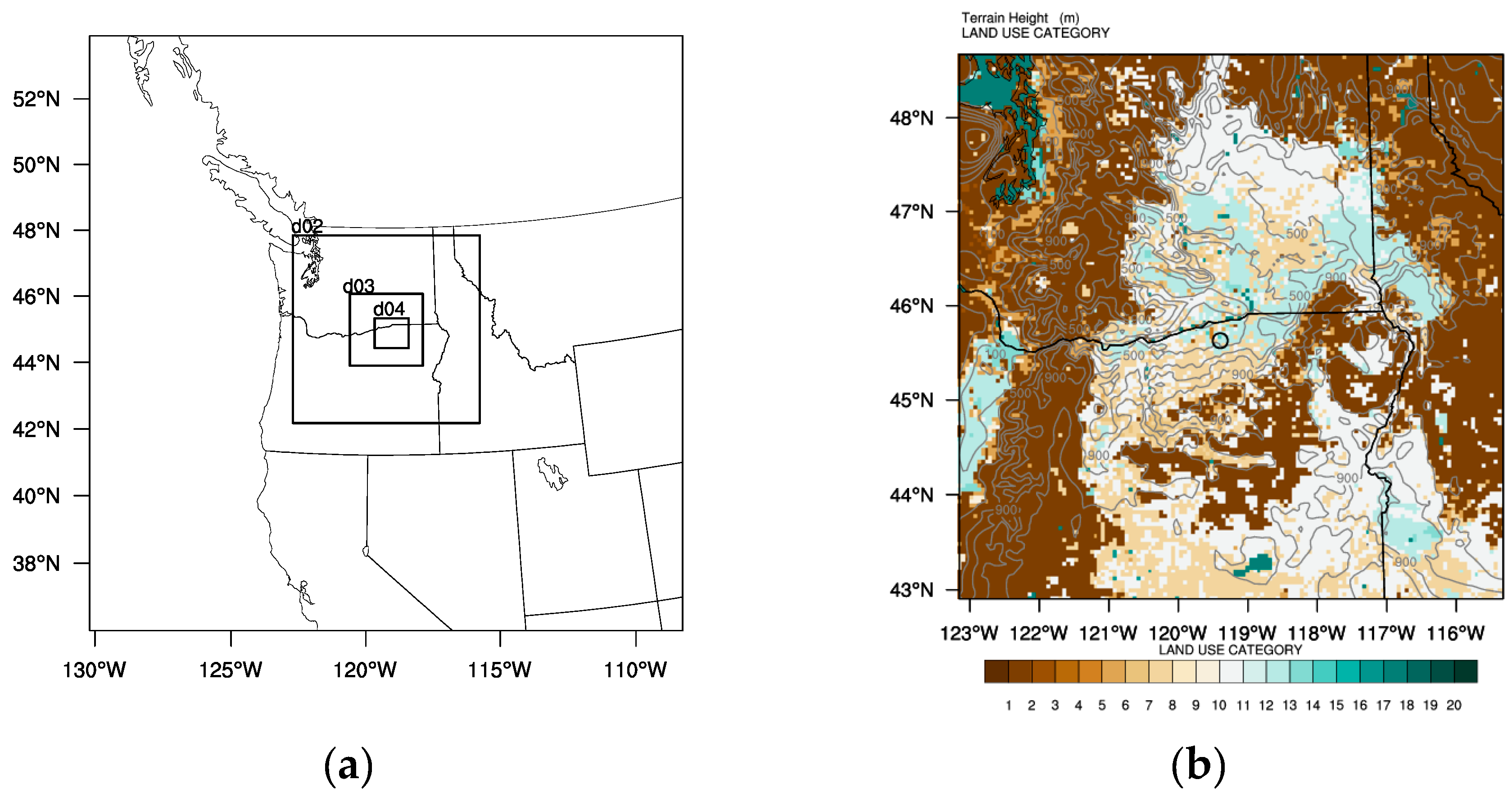
WRF (version 3.7.1) was configured with four two-way nested domains using horizontal resolutions of 13.5, 4.5, 1.5, and 0.5 km. Domain 1 covers the western part of North America (37–53° N, Figure 1). Domain 2 covers the states of Oregon, Washington, and western Idaho. The spatial distribution of land-use category and terrain height over the second domain is shown in Figure 1. The innermost domain (d04) is centered around the observation site and has an area of 11,608 km2 with a 231 × 201 grid dimension. Inner domain boundary conditions were provided from the adjacent outer domain. The simulated friction velocity, sensible heat flux, and latent heat flux of the innermost domain were compared to the flux tower observations to ensure the benefit of high resolution model results. The second domain was used to study the WRF performance on simulations of surface meteorology variables (T2, Q2, and WS10) to ensure there were enough weather stations included for comparison (Table 2). The second domain was also used to study the spatial distribution of sensible and latent heat fluxes to include the land-use effects on the turbulent heat fluxes. The observation site was classified as dryland, cropland, and pasture in the U.S. Geological Survey (USGS) dataset and cropland in the Moderate Resolution Imaging Spectroradiometer (MODIS) dataset, with the dominant soil category as silt loam. The model was initialized at 0000 UTC 21 September 2014, where the first 32 h were considered as the model spin-up period and removed from subsequent analyses. Forty-five vertical terrain-following levels, extending to 100 hPa, were employed in all domains with increased resolution in the lowest part of the boundary layer (i.e., nine layers below 1 km). The middle level of the lowest model layer height was 10.5 m above ground. A previous study found that the WRF model simulated surface meteorology parameters were not sensitive to the lowest model level height in unstable conditions and became sensitive when the lowest model height was below 40 m during stable conditions [32].
Four-dimensional data assimilation (FDDA) was applied to wind, moisture, and temperature in the outer two domains in all WRF runs except for one sensitivity run [NAM-ACM2-U(No-nudge)]. FDDA was implemented for horizontal wind components in all layers and for temperature and water vapor mixing ratio at the surface and above the PBL. The National Centers for Environmental Prediction (NCEP) Administrative Data Processing (ADP) Global Surface Observational Weather Data (ds461.0) and Upper Air Observational Weather Data (ds351.0) with 6-hourly temporal resolution were used for FDDA. The objective analysis tool Obsgrid [34] was used to enhance the FDDA analysis using the observation datasets mentioned above and to provide the data (combination of observations and re-analysis data for air T and Q) used for the indirect soil nudging scheme in PX LSM [17].
Different land-use datasets can cause solar energy absorption variations, leading to simulation discrepancies of meteorological conditions, including surface fluxes and PBL processes. Therefore, USGS and MODIS land-use datasets were used in the simulations to investigate land-use impacts on the WRF model performance (NAM-ACM2-U and NAM-ACM2-M). Updated land-use datasets can be beneficial to NWP model accuracy. USGS and MODIS were chosen because they are two widely-used land-use datasets in WRF (NAM-ACM2-U and NAM-ACM2-M). The USGS dataset was collected from 1992 to 1993. The MODIS dataset is a satellite product and represents land use in 2004 [35]. Both rely on lookup tables for the land use information and do not offer dynamic land use information to model the land surface processes.
Mesoscale climate models are sensitive to large-scale input forcing fields [36]. Hence, NAM and NARR datasets were used for model initial and boundary conditions and their corresponding simulation results were compared. Large-scale forcing datasets with higher spatial resolution are expected to produce more realistic meteorology variables in NWP models. NAM-ACM2-U and NARR-ACM2-U were designed to test the WRF sensitivity to NAM (12 km, 6 h) and NARR (32 km, 3 h) datasets.
The LSMs calculate the surface fluxes in models with exchange coefficients from surface layer schemes, and Noah LSM and PX LSM were investigated in this study. Correspondingly, WRF was run with three different PBL schemes (ACM2, YSU, and MYJ), which were coupled with the proper LSM, to study the features of PBL physics influence on WRF results. ACM2 was coupled with the PX LSM and YSU and MYJ were both coupled with the Noah LSM. The PX LSM, because of the indirect soil temperature and moisture nudging schemes, is expected to perform better than other LSMs. The PX LSM soil nudging was applied in the outer two domains. NAM-ACM2-M, NAM-YSU-M, and NAM-MYJ-M were conducted to compare the PX LSM and the Noah LSM performances, as well as the PBL scheme performances (ACM2, YSU, and MYJ).
Initially, only six model configurations were selected to examine the sensitivity of large-scale forcing datasets and PBL schemes. However, after analyzing the results it became clear that the NARR data had significant impacts on the surface flux results and therefore two additional simulations were added to the experiment to compare the NARR results paired with the MYJ and YSU PBL schemes with the ACM2 PBL results. Therefore, eight WRF scenarios in total were designed to conduct the sensitivity experiments, denoted as NAM-ACM2-U(No-nudge), NAM-ACM2-U, NARR-ACM2-U, NAM-ACM2-M, NAM-YSU-M, NAM-MYJ-M, NARR-YSU-M, and NARR-MYJ-M. The details for each scenario are summarized in Table 1. The common set of other physics options in the sensitivity experiments includes the Morrison double-moment scheme for microphysics [37], Rapid Radiative Transfer Model longwave radiation scheme [38], Dudhia shortwave radiation scheme [39], and the Kain-Fritsch scheme for cumulus parameterization [40].
Different from the observation data, where the friction velocity and sensible and latent heat fluxes are directly quantified using the EC method, the WRF model relies on parameterizations to simulate these turbulence variables. Specifically, surface layer schemes are based on Monin-Obukhov similarity theory (MOST), from which the transfer coefficients of momentum, heat, and moisture are calculated. For example, PX, revised MM5-similarity, and Eta similarity surface layer schemes all employ Monin-Obukhov similarity theory, and details on scheme development can be found in Pleim [41], Jiménez and Dudhia [42], and Janjić [43], respectively. The surface meteorological parameters at their routine observation heights, such as T2, Q2, and WS10, are calculated using similarity theory [44]. WRF simulated friction velocity () is formulated as:
where k is the von Kármán constant, L is the Monin-Obukhov length scale, represents the roughness height, z denotes the height above the ground, is the function for stability correction [45], and U is the wind speed in the lower layer.
Surface heat fluxes, sensible heat flux (H) and latent heat flux (LH), are calculated in the LSM as:
where ρ is the air density, cp is the specific heat of air at constant pressure, and U is the wind speed. θ is the potential temperature and q represents the humidity. The subscripts a and g stand for the first model layer and ground surface, respectively. Ch represents the transfer coefficient of heat. The exchange coefficient directly impacts the coupling strength of the land and atmosphere interactions in WRF [14]; λ is the latent heat of evaporation of water. E is evapotranspiration, which relies on parametrizations of soil moisture and stomatal resistance [13,34]. Details on the difference between Noah and PX LSM can be found in Miao, Chen and Borne [20].
2.3. Evaluation Methods
The METSTAT program [46] was used to evaluate the model performance in simulating T2, Q2, WS10, and 10-m wind direction (WD10) with the TDL datasets. Mean bias (MB), root mean square error (RMSE), and index of agreement (IOA) [47] were calculated:
where N is the total sampling number over space and time; i is each grid point; P and O represent predicted and observed value, respectively. The range of values for IOA is 0 to 1, where 1 implies perfect agreement. These evaluation metrics were chosen because they are commonly used statistical metrics in NWP model performance evaluation [48]. METSTAT was run for the second domain (4.5 km resolution) to increase the number of measurement locations in the TDL dataset for the statistical evaluation compared to the inner two domains. Measurements from 72 surface observation sites from the TDL dataset were available in the second domain for evaluation.
Mean absolute error (MAE) is also used to describe the average difference between simulated and observed friction velocity and sensible and latent heat fluxes:
The MAE, rather than the IOA, is used here because of MAE’s greater sensitivity to model errors in simulating the turbulence variables in our case study. The i is each time stamp. In Equation (7), the predicted value (P) is the WRF results of the nearest grid point to the flux tower in the innermost domain. The observed value (O) is the turbulence data measured by the flux tower.
3. Results
3.1. Surface Meteorological Variables
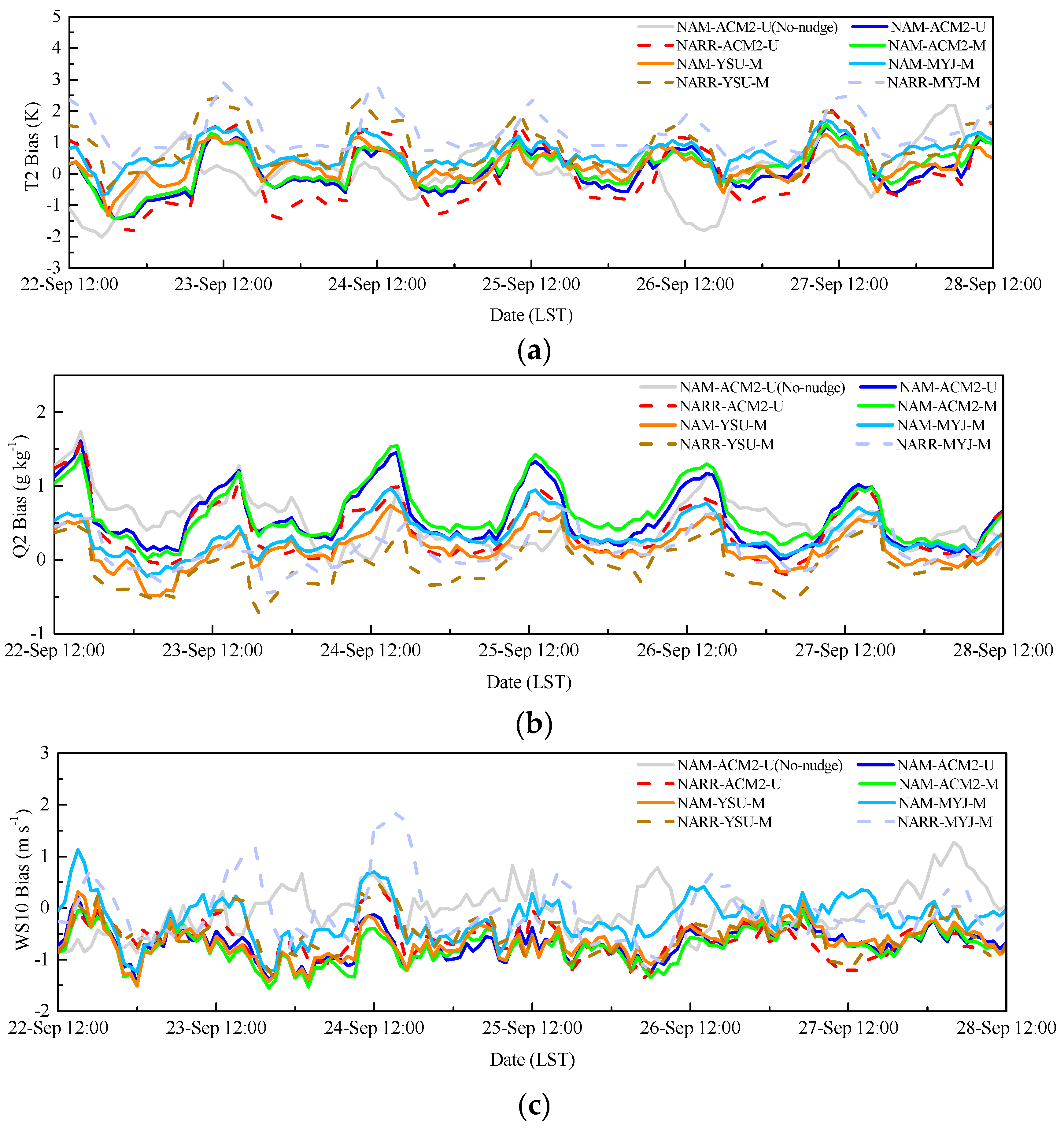
Table 2 provides the summary of the statistical results (MB, RMSE, and IOA) for the simulated surface meteorological variables from the eight WRF sensitivity experiments for the second domain from 22 to 28 September. The mean observational values of T2, Q2, and WS10 from TDL datasets were 289.26 K, 8.36 g kg−1, and 3.22 m s−1, respectively. The MB indicates that all scenarios exhibited a warm bias for T2, an over-prediction for Q2 (except for NARR-YSU-M), and an under-prediction for WS10 on average. The MB for WD10 ranged from 4.39 to 8.27 degrees for the WRF simulations. The average IOA of WRF simulations was highest for T2 (0.94) and lowest for WS10 (0.68). For the FDDA sensitivity testing, NAM-ACM2-U had obvious improvements in simulated T2, Q2, and WS10 with reduced RMSE and increased IOA compared to NAM-ACM2-U (No-nudge).
3.1.1. Surface Temperature
The ACM2 with nudging case (NAM-ACM2-U) improved model performance for T2 by producing a lower RMSE than NAM-ACM2-U(No-nudge) by 21%, which is consistent with Otte [49] who found that FDDA improves meteorological simulations. All scenarios with nudging produced a warm bias during the daytime and a cold bias at nighttime, except for the cases of NARR-YSU-M and NARR-MYJ-M. Overall, T2 was overestimated in these two cases, where NARR-MYJ-M produced the largest mean bias for T2 among the runs (Table 2). The NAM forcing dataset performed better than NARR for T2 with a 16% lower RMSE and 2% higher IOA on average. Compared with the NAM-ACM2-U experiment, the NAM-ACM2-U(No-nudge) RMSE was higher by 26%, NARR-ACM2-U RMSE was higher by 11%, and NAM-ACM2-M RMSE was higher by 6%. The RMSEs and IOAs were similar among the PBL comparison scenarios for NAM-ACM2-M, NAM-YSU-M, and NAM-MYJ-M. Overall, NAM-ACM2-U performed best in simulating T2 and had the lowest RMSE and highest IOA.
Analysis of the average hourly variation of MB indicated that the NAM-ACM2-U(No-nudge) experiment was out of phase with the other scenarios (Figure 2), which all had the largest over-predictions during daytime at around 1000 LST, indicating a time dependence of the MB. The averaged diurnal variation of T2 bias showed that NARR-MYJ-M had the least agreement with T2, excluding the NAM-ACM2-U(No-nudge) experiment. NARR-MYJ-M produced the largest warm bias (2.45 K) at 1000 LST, which was consistent with it having the second highest RMSE in Table 2.
3.1.2. Surface Water Vapor Mixing Ratio
In terms of MB, all WRF scenarios overestimated Q2 by approximately 0.16 to 0.61 g kg−1, except for NARR-YSU-M (Figure 2). The RMSE ranged from 0.83 to 0.99 g kg−1 except in NAM-ACM2-U(No-nudge) case, which had the largest RMSE (1.30 g kg−1). The mean hourly variations of MB were similar in all scenarios, exhibiting over prediction for Q2 with a peak value (average of 1.03 g kg−1) at around 1600 LST, except for NAM-YSU-M. The comparison showed that the maximum differences among the simulations were during the daytime, which was also found in Hariprasad, et al. [50]. It is noteworthy that even though NARR has coarser spatial resolution compared with NAM, it has finer temporal resolution (3 h). The MODIS land-use dataset did not improve Q2 statistics in terms of RMSE and IOA. The YSU PBL scheme coupled with Noah LSM (NAM-YSU-M) outperformed the other scenarios in simulating Q2.
3.1.3. 10-m Wind Speed
All simulations were in phase with each other and showed a consistent underestimation of WS10 during nighttime (Figure 2). The average daily variation of WS10 from 22 to 28 September exhibited an over-estimation of wind speed for MYJ PBL schemes (NAM-MYJ-M and NARR-MYJ-M) between 1000 LST and 1600 LST with a maximum bias of 0.8 m s−1. Simulated WS10 from ACM2 and YSU PBL schemes was smaller and closer to observations compared with MYJ. This indicates that the non-local PBL schemes (ACM2 and YSU) produced more realistic surface winds under unstable conditions in the daytime compared with the local scheme (MYJ). The local closure PBL scheme suffers from over-simplification of representing the vertical turbulent mixing by the large eddies in the PBL and thus underperforms compared to the non-local schemes during convective conditions. NAM-ACM2-U produced the lowest RMSE (1.56) and NAM-MYJ-M had the highest IOA (0.74) among all the scenarios. The statistics showed that in comparison with NARR cases, WRF runs using the NAM input forcing data with a finer spatial resolution (12 km) had better agreement with WS10 observations. This is consistent with the result from Lu and Zhong [8] when modeling a persistent cold air pool event in Utah.
3.2. Turbulence Data
3.2.1. Temporal Variation of Surface Fluxes
Simulated friction velocity (u*), sensible heat flux, and latent heat flux from the eight WRF scenarios were compared at the nearest grid to the flux tower observation site (Figure 3). Observations are also presented for comparison. Mean u* measured from the flux tower during the observation period was 0.18 m s−1, with peak values observed in the daytime. Simulated u* was overpredicted in all WRF scenarios by 0.04 m s−1 on average (Table 3), among which NAM-YSU-M overestimated it to the largest degree (40%). The simulated u* from WRF is calculated from wind speed and stability functions in the surface layer schemes. Since simulated near surface wind speed during the observation period was underestimated in NAM-YSU-M (Figure 2), this overestimation of u* is related to the MOST scaling being used to derive the stability functions and the corrected stability functions in the revised MM5 surface layer scheme which is tied to the YSU PBL scheme. NAM-MYJ-M performed better for u* than NAM-YSU-M in terms of RMSE, although with similar temporal variability. This is consistent with the case study on turbulent flow parameters in a dry convective boundary layer using WRF by Gibbs, Fedorovich and Eijk [3]. NARR outperformed NAM in simulating u* with 14% lower RMSE and 15% lower MAE. Considering the higher RMSE using NARR in simulating WS10 (Table 2), this preference of NARR in simulating u* might be a coincidence. NARR-MYJ-M performed best among the WRF scenarios with the lowest RMSE and MAE. The u* for the NAM-ACM2-U and NAM-ACM2-M cases exhibited almost the same temporal variation and magnitude, indicating that land-use datasets had a negligible influence on the simulation of the surface layer shear stress at the flux tower site.
The temporal variations of sensible heat fluxes were similar in all WRF scenarios and the observational dataset (Figure 3), except that on average the value simulated by WRF was up to two times larger than the observations (NARR-YSU-M). The sensible heat flux simulated by WRF was as large as 322.7 W m−2 (from NAM-YSU-M), where the largest observed value was 175.1 W m−2. Simulation discrepancies among the WRF scenarios were largest during the time period associated with peak solar heating. NAM-ACM2-M produced smaller sensible heat fluxes, which was closer to observations compared with NAM-YSU-M and NAM-MYJ-M. This can be attributed to the indirect nudging for temperature in the PX LSM used in NAM-ACM2-M. The lower positive bias of T2 in NAM-ACM2-M (Table 2) was related to the reduced sensible heat flux compared with NAM-YSU-M and NAM-MYJ-M. The value of sensible heat flux from NAM-MYJ-M was up to two times larger than that from NAM-ACM2-M. NAM-ACM2-U simulated the lowest peak value of sensible heat flux of all cases and showed better performance in simulated sensible heat flux than NARR-ACM2-U based on a smaller RMSE (Table 3), indicating improvement by using NAM versus NARR. The same conclusion could also be made based on the Noah LSM cases (NAM-YSU-M and NARR-YSU-M, NAM-MYJ-M and NARR-MYJ-M). The NAM-YSU-M and NAM-MYJ-M scenarios used the same Noah LSM, suggesting that the only difference between them was the PBL and surface layer scheme. Sensible heat flux simulated using NAM-YSU-M showed less agreement with observations than that from NAM-MYJ-M. There was increased soil moisture when there was watering for irrigated farmland nearby at around 0800 LST 24 September and around 1400 LST on 25 September, which was not reflected in the NAM or NARR initialization data, or simulated by the WRF model. Thus, less surface available energy would be partitioned into sensible heat flux due to irrigation. This could somehow contribute to the overestimation by WRF results compared to observations, and will be further investigated by comparing the simulated and observed latent heat fluxes.
The PX LSM was expected to produce better simulations of latent heat flux due to its soil moisture nudging. The runs with the ACM2 PBL scheme using NAM, though with positive bias, captured the daily variation of the latent heat flux. However, during the daytime (0600 LST~1800 LST), the scenarios using the PX LSM produced higher latent heat flux values than the observations by 46.1 W m−2 on average, with differences as large as 285.4 W m−2 (Figure 3). The overestimations of the latent heat flux in runs using PX LSM reached their peak at around 1200 LST 26 September and were much larger than other time periods. Latent heat flux was underestimated by 28.1 W m−2 in Noah LSM cases using the NAM dataset (NAM-YSU-M and NAM-MYJ-M) and was less consistent with the temporal variation patterns of the observed fluxes than those using the PX LSM. The WRF cases using NARR produced more realistic latent heat fluxes than cases using NAM, with a 27% lower RMSE and 19% lower MAE on average. Noah latent heat fluxes were improved with a 57% lower RMSE compared to Pleim-Xiu, when NARR forcing data was used. The better performance of Noah LSM in simulating latent heat flux is expected considering its better performance in simulating Q2 (Table 2). This indicates that the soil moisture nudging in PX LSM is not as effective as its soil temperature nudging. This was also found by Gibbs, Fedorovich and Eijk [3], where soil moisture simulated by the Noah LSM was in better agreement with observations compared to the PX LSM in a case study over the Great Plains. It was found that NAM-ACM2-M produced more realistic latent heat fluxes than NAM-ACM2-U in terms of RMSE (Table 3).
3.2.2. Spatial Variation of Surface Fluxes
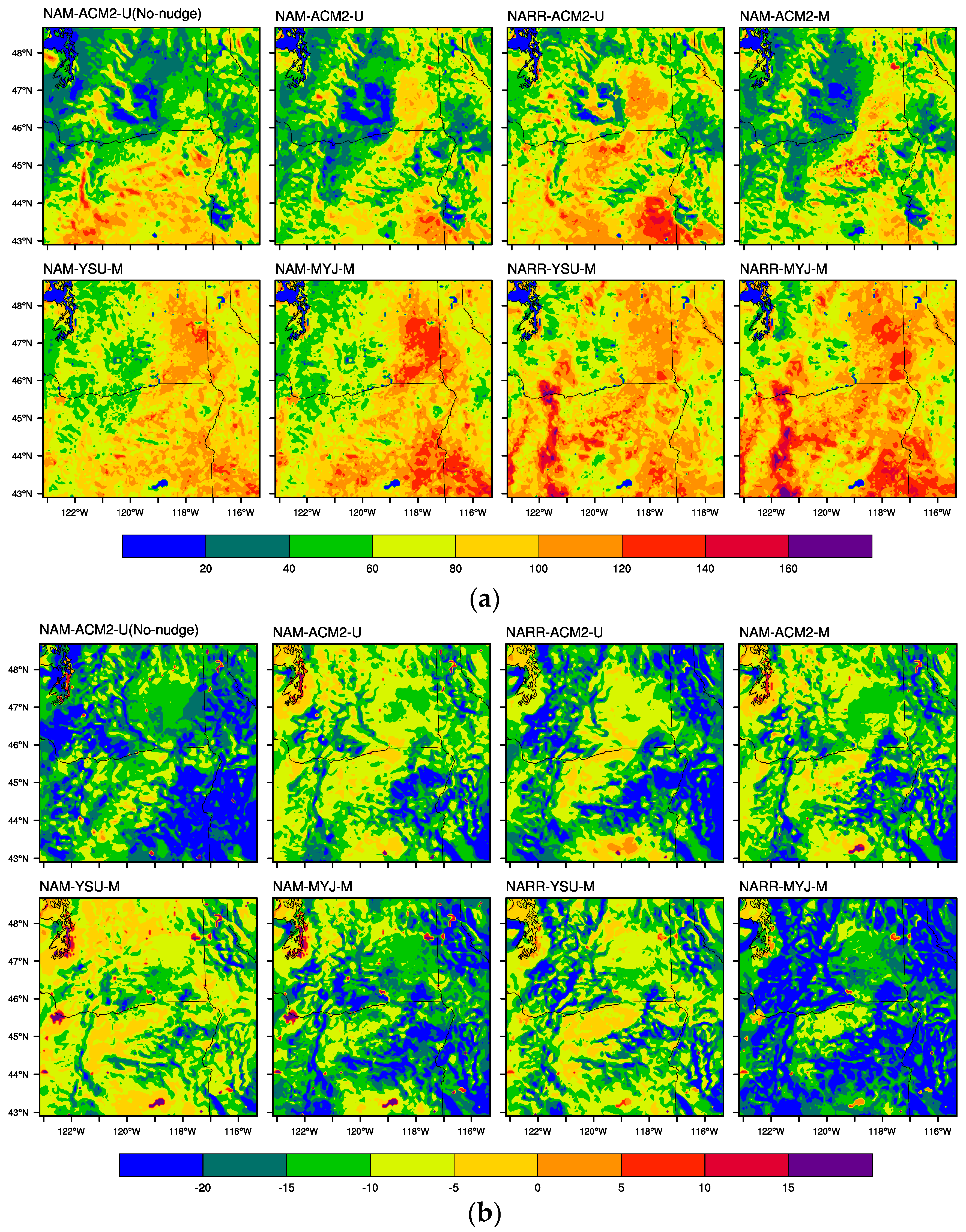
The average spatial variations of simulated sensible and latent heat fluxes in the daytime and nighttime were analyzed for the second domain to examine the differences induced by land-use datasets, large-scale forcing datasets, LSMs, and PBL schemes regionally (Figure 4). In the daytime, the maximum values of sensible heat flux occurred for the NARR-MYJ-M case in the western part of Oregon. In comparison with the nudging case of NAM-ACM2-U, the NAM-ACM2-U(No-nudge) predicted higher sensible heat flux, especially in central Oregon. It was evident here that the NARR cases produced higher sensible heat fluxes than the NAM cases. The MYJ PBL scheme produced higher sensible heat flux than the YSU and ACM2, especially over southeast Washington. The PX LSM runs produced lower minimum sensible heat fluxes over north-central Washington than scenarios run with Noah LSM. During nighttime, the non-local YSU PBL scheme predicted higher sensible heat fluxes than the MYJ and ACM2.
Figure 4 suggests that the latent heat flux distribution pattern in the daytime was impacted by the land-use distribution seen in Figure 1. Higher values of latent heat flux were present over the areas dominated by several kinds of forests, contributing to more surface energy being partitioned into evaporation and transpiration. This was also shown by LeMone et al. [11] where the maximum observed latent heat flux was over areas with green vegetation. Spatial variation of the predicted top layer soil moisture from the eight WRF experiments also influenced surface heat fluxes, where larger latent heat fluxes occurred in areas with higher soil moisture. Simulated latent heat fluxes from NAM-YSU-M were the smallest among the WRF experiments, in contrast to the largest value from NARR-ACM2-U. The scenario using the MODIS land-use dataset (NAM-ACM2-M) produced almost identical latent heat flux spatial distributions and magnitudes to the scenario using USGS (NAM-ACM2-U), but predicted slightly higher mean latent heat fluxes over northeastern Oregon. Latent heat fluxes from NARR cases run with Noah LSM were mostly higher over forested areas than heat fluxes from NAM cases. While NARR-ACM2-U produced larger latent heat fluxes than NAM-ACM2-U over nearly the whole domain. It was found that latent heat fluxes simulated by NAM-MYJ-M were about twice the value of those using NAM-YSU-M for forested areas. At the nighttime, the impacts of land use distribution on latent heat flux distribution were not as significant as the daytime. The ACM2 PBL scheme produced higher latent heat fluxes than the YSU and MYJ for both the daytime and nighttime. Future studies should investigate the spatial variability of the surface fluxes using multiple flux towers to determine the impact of land cover type.
3.3. Vertical Structure
The simulated PBL heights and vertical profiles of potential temperature and moisture were compared to further examine the influence of land-use datasets, large-scale forcing datasets, LSMs, and PBL schemes on vertical turbulence. In WRF, the PBL height is calculated using different methods for each PBL scheme. Since simulated PBL height variations may arise from the different calculation methods in each of the PBL schemes [48], a unified method of calculating the PBL height is more valuable for comparing model results. The bulk Richardson number (Rib) method defines the PBL height as the level at which the Rib reaches a critical value. The Rib is calculated as follows
where θv is the virtual potential temperature; U is the horizontal wind speed; subscript H and s represents the level of H (where H is the height) and the lowest model level (surface level) zs, respectively. Based on previous studies, the critical Rib varies from 0.15 to 1.0 [51]. However, the study of the optimal Rib is out of scope of this research and the bulk Rib method with a critical value of 0.25 [45] was used here to diagnose the PBL height for each WRF simulation to ensure consistency in comparison.
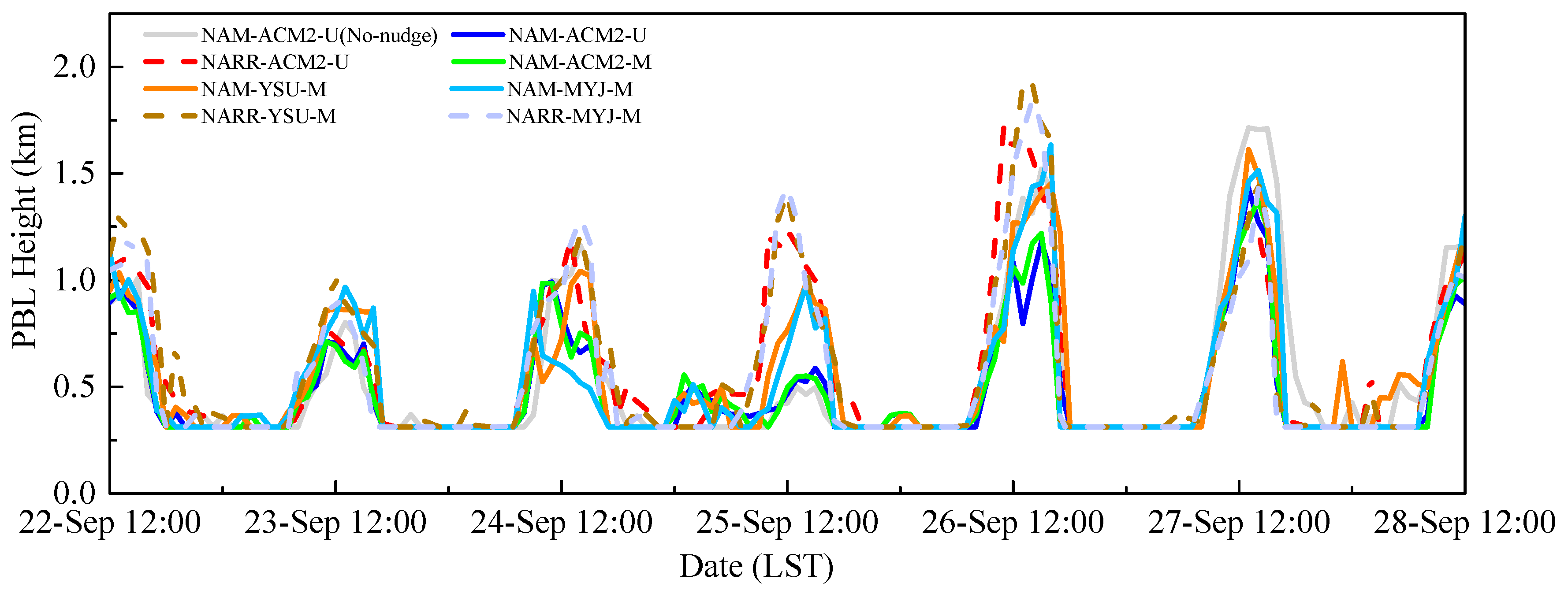
Here, PBL heights calculated with the bulk Rib method were analyzed. Simulation derived PBL heights (Mean Sea Level, MSL) increased after sunrise, with a peak value (mean of 1.09 km) at around 1400 LST (Figure 5). Among the eight WRF scenarios, the NARR cases predicted higher mean PBL height over the flux tower site than the NAM, especially in the daytime. Since NARR produced higher Rn than NAM, deeper convective mixing was produced for NARR cases because of more thermal surface heating to the atmosphere, leading to a lower PBL height for NAM cases. For runs with NAM large-scale forcing dataset, the YSU PBL scheme, which produced larger simulated sensible heat flux, diagnosed higher PBL height compared to ACM2 and MYJ on average. The ACM2 scheme predicted the lowest PBL height in the daytime and MYJ gave the lowest during nighttime. The simulated sensible heat flux in NAM-ACM2-M was less than that in NAM-YSU-M and NAM-MYJ-M (Figure 3), indicating less surface turbulent mixing in the PX LSM in the daytime. Except for NAM-ACM2-U(No-nudge), the WRF scenarios predicted elevated PBL height with an average of 0.41 km during the night on 24 September.
To investigate the PBL entrainment differences among the eight WRF scenarios, moisture and temperature vertical profiles were inspected. Figure 6 illustrates the predicted vertical variation of potential temperature and water vapor mixing ratio over the flux tower site averaged at 0900, 1500, and 0300 LST, corresponding to the morning, afternoon, and nighttime, respectively. There was more variability in simulation results for moisture than potential temperature. Temperature profiles exhibited a more similar shape and magnitude. NAM-ACM2-U(No-nudge) produced higher moisture values below 1.9 km and lower potential temperature than NAM-ACM2-U at 1500 LST, indicating that the FDDA nudging method also influenced the PBL structure. The profile difference extended above the top of the PBL. Different land-use datasets resulted in negligible discrepancies in the vertical profiles (NAM-ACM2-U and NAM-ACM2-M). The impacts of large-scale input forcing datasets on the PBL structures were largest at 1500 LST, around the time when PBL height reached the highest value. NARR produced higher temperature and lower humidity at 1500 LST than NAM from the surface to about 2 km.
At 0900 LST, NAM-MYJ-M simulated a higher moisture than NAM-YSU-M near the surface. Due to the weaker mixing process of the local PBL scheme [26,50], the moisture from NAM-MYJ-M was lower than NAM-YSU-M above 2 km. Based on the moisture profile at 1500 LST, the mixing in NAM-ACM2-M was shallower than that in NAM-YSU-M near the surface, which is consistent with the inter-comparison results of PBL parameterizations from a prior study [25]. After sunset, NAM-YSU-M simulated a drier and slightly warmer layer than NAM-MYJ-M, which could be attributed to the stronger mixing in the YSU PBL scheme.
Under the convective conditions at 1500 LST, the potential temperature profiles showed a uniform distribution up to around 1 km and then increased with height. This indicated the time evolution of PBL after 0900 LST, with a thicker mixing layer from NAM-YSU-M compared with NAM-ACM2-M and NAM-MYJ-M. Diurnal variation of mixing was also reproduced from the humidity profiles at 1500 LST, characterized by a nearly unvarying distribution from the surface to the top of PBL. Stable conditions at nighttime (0300 LST) were simulated by the WRF runs with similar potential temperature vertical profiles. Comparison with sounding data in future studies is necessary to assess the model performance on the vertical transport and entrainment simulations.
4. Discussion
Our two objectives, analyzing the WRF performance on simulating surface meteorology and turbulent fluxes and their sensitivity to input datasets and physics configurations, were addressed through the eight WRF sensitivity experiments. The results shown above illuminate discrepancies in model performance, where often times NWP models are able to simulate one property well (e.g., temperature) while experiencing pitfalls in the ability to simulate other variables (i.e., latent heat flux). This type of investigation is important because there are limited datasets available to evaluate the variables that NWP models have the most uncertainty in, such has surface heat fluxes. The following discussion aims to elucidate the details contributing to these discrepancies in results from the WRF sensitivity experiments.
4.1. LSMs Sensitivities to Large-Scale Forcing Datasets
The Noah LSM was more sensitive to the large-scale input forcing dataset than PX LSM in our case, suggesting that the differences between NARR and NAM in simulating T2 were larger for the Noah LSM (Table 2). The indirect soil temperature nudging scheme in the PX LSM minimizes the impacts of the potential bias introduced by input forcing datasets. The NARR cases simulated Q2 better than the NAM cases when run with the PX LSM, whereas the preference went to NAM when running with Noah LSM. This suggests that there is a sensitivity of LSMs performance to large-scale input forcing datasets in NWP models for simulation of surface meteorological variables. Additionally, LSMs that implement soil nudging schemes behave differently than LSMs without soil nudging because the large-scale input forcing datasets determine which data is available for the soil nudging and the quality of the data. Therefore, since the PX LSM model was the only LSM in this sensitivity experiment to use any sort of soil nudging scheme, it makes sense that it behaved differently than the Noah LSM and was less sensitive to the selection of large-scale forcing data. These discrepancies in soil moisture also impact the surface energy balance and will be discussed in more detail below.
4.2. Simulation Differences for Surface Energy Balance
The positive bias of sensible heat flux can arise from the bias of the simulated surface radiation budget, which further impacts the partitioning of surface available energy [52]. To investigate this impact on the simulation results, time variations of simulated Rn were plotted to see differences in the simulated surface fluxes among WRF runs (Figure 7). The magnitude and temporal variation of Rn from each WRF sensitivity run was similar, with maximum values in the range of 396–452 W m−2. The largest influence came from the different large-scale forcing datasets, where NARR produced 16% higher Rn on average than NAM at the flux tower site. Additional discrepancies arise from the LSM, where simulations using the Noah LSM produced 6% lower Rn on average during daytime than those with the PX LSM. If the differences in the simulated sensible heat fluxes were solely caused by these differences in Rn, the ratio of sensible heat flux to Rn for each WRF sensitivity run would be the same. However, the ratios were different, and the average ratio ranged from 0.19 (NAM-ACM2-U) to 0.65 (NARR-YSU-M) during daytime. This reveals that the difference among the simulated surface fluxes was not entirely related to uncertainties in the radiation modeling and may be partially attributed to the partitioning of surface available energy. However, this study is limited because we do not have radiation observations to compare with the model results. Therefore, future experiments should quantify the radiation balance at the surface to do a full investigation of these uncertainties in WRF.
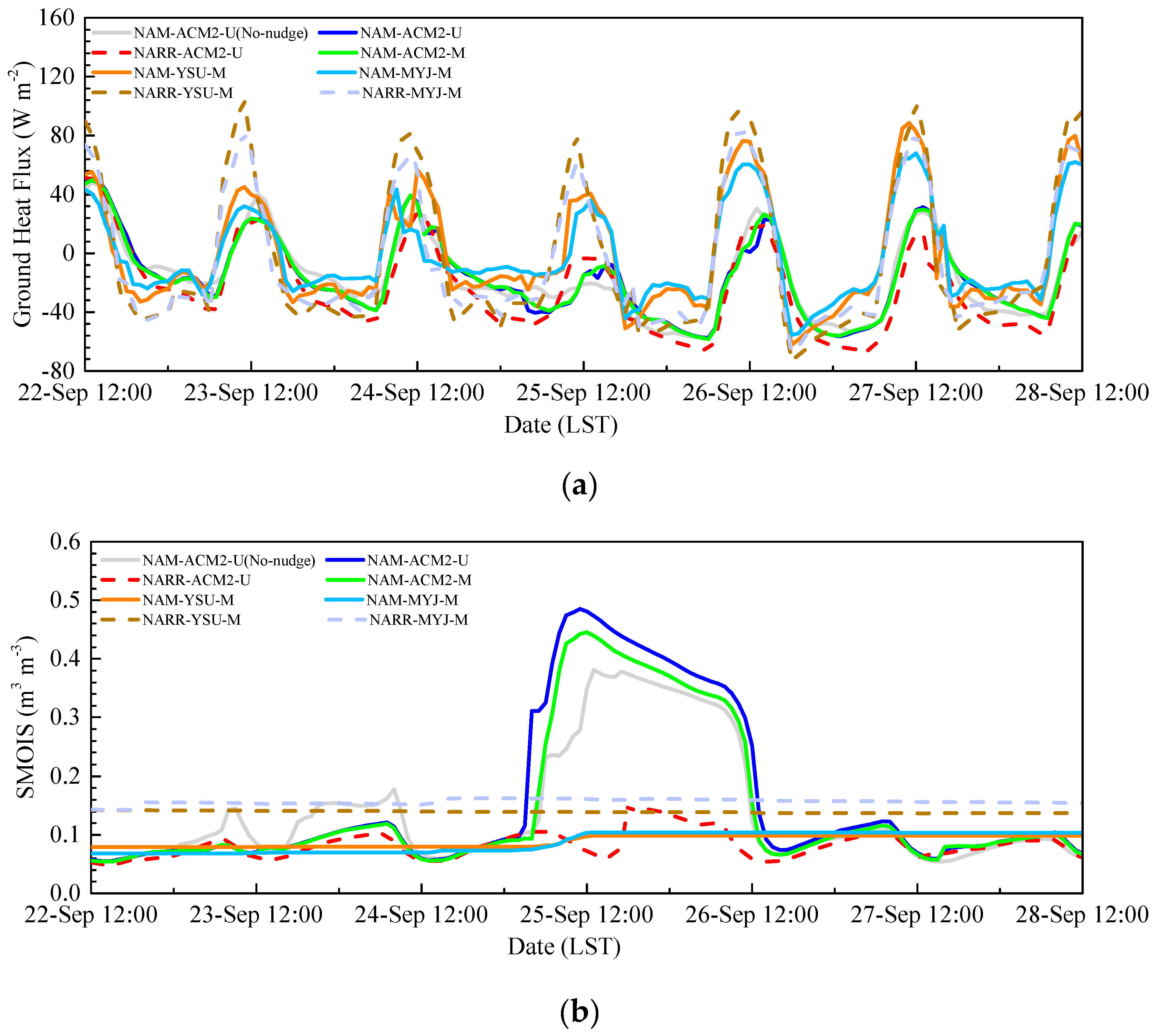
Based on the surface energy balance, the net radiation equals to the sum of ground heat flux, sensible heat flux, and latent heat flux [53]. Therefore, in addition to the modeled net radiation the time series of simulated ground heat flux was investigated to assess its influence on the simulation discrepancies (Figure 8, with no corresponding observation data available). NARR cases produced 33% higher ground heat flux on average than NAM during the daytime when using Noah LSM, whereas NAM cases gave higher values than NARR when run with PX LSM. It is seen that ground heat flux in runs using the Noah LSM was higher than those using PX LSM, with the Noah LSM results having a similar magnitude of ground heat flux compared to the sensible and latent heat fluxes. Whereas, the PX LSM ground heat fluxes were smaller in magnitude than both the sensible and latent heat fluxes. In the daytime, ground heat flux from the Noah LSM simulation was up to 97 W m−2 larger than that from the PX LSM results. Thus, the impact of ground heat flux simulation difference on the sensible and latent heat flux simulation difference is largest during the daytime but is still less significant than the partitioning of surface available energy.
In addition to ground heat flux soil moisture impacts the net surface energy budget and leads to evapotranspiration at the surface, and impacts the latent heat flux directly. The initial top layer soil moisture (1 cm depth in PX LSM and 10 cm depth in Noah LSM) was consistent among the WRF scenarios (Figure 8). The NARR-ACM2-U scheme simulated the soil moisture about 48% less than NAM-ACM2-U on average, with a maximum difference of 0.41 m3 m−3 produced during the soil moisture augmentation period on 25 September. The increases of soil moisture were related to precipitation simulated by WRF scenarios. Not all WRF runs simulate rain on September 25 and all the runs simulate different amounts of precipitation. Runs with NARR produced less precipitation than the NAM. The soil moisture remained the same in NARR-YSU-M where no precipitation was simulated (figure not shown). The NAM-ACM2-M scheme had an almost identical soil moisture evolution as NAM-ACM2-U, except with a slightly higher peak during the moisture swell stage. This implies that the differences in simulating soil moisture using different large-scale input forcing data were larger than those related to different land-use datasets. The Noah LSM had less diurnal latent heat flux and soil moisture variability than the PX LSM (Figure 3). Modeled soil moistures from the Noah LSM runs using NARR (NARR-YSU-M and NARR-MYJ-M) were higher than those using NAM (NAM-YSU-M and NAM-MYJ-M), resulting in higher latent heat flux values that were closer to the observations. This indicated that the large-scale input forcing data had a large impact on the simulated latent heat flux in runs using Noah LSM, where the NARR data simulated higher Rn and more soil moisture (versus NAM) and therefore improved the simulated latent heat fluxes when compared to observations. Due to the PX LSM indirect soil moisture nudging, the NAM-ACM2-M scheme produced a higher soil moisture enhancement and a faster depletion evolution than NAM-YSU-M and NAM-MYJ-M, therefore the larger latent heat flux in PX LSM (NAM-ACM2-M) contributes to a higher mean bias of Q2 than Noah LSM (NAM-YSU-M and NAM-MYJ-M) (Table 2).
5. Conclusions
Eight WRF simulations with different large-scale input forcing (NAM and NARR), land-use category datasets (USGS and MODIS), LSMs (PX and Noah LSM), and PBL schemes (ACM2, YSU and MYJ) were run to investigate their impacts on modeled surface turbulent fluxes and PBL structures. Impacts of observational nudging schemes were also evaluated. The sensitivity experiments were conducted using WRF v3.7.1 and evaluated using the TDL surface hourly observation dataset and flux tower field experiment data spanning over seven days from a site surrounded by farmlands. Through comparisons with observations, the WRF uncertainties in simulating surface meteorology parameters and surface turbulent fluxes were evaluated. Additionally, the sensitivity to input datasets and physics schemes were investigated by intercomparisons among the WRF sensitivity experiments results.
Overall, the WRF scenarios over-predicted the 2-m temperature and 2-m humidity, whereas they provided a negative bias in the 10-m wind speed compared with the observation dataset over the second domain. The application of the FDDA scheme significantly improved the simulation of surface meteorological parameters, including temperature, humidity, and wind speed. NAM (12 km, 6 h) better simulated surface meteorology parameters compared with NARR (32 km, 3 h) except when using PX LSM to simulate humidity. The Noah LSM was more sensitive to large-scale input forcing dataset than PX LSM in our case. Compared with USGS, the application of the MODIS land-use dataset was not found to perform better with respect to surface meteorology fields in this case. Better performance in simulating T2 was seen for runs using the PX LSM, where the soil temperature and moisture nudging method was applied. Simulated surface temperature was sensitive to PBL schemes. The YSU PBL scheme (NAM-YSU-M) produced better 2-m temperature simulation compared with the MYJ (NAM-MYJ-M) scheme. Non-local PBL schemes (ACM2 and YSU) produced more realistic surface winds under unstable conditions in the daytime compared with the local closure PBL scheme (MYJ).
Simulated friction velocity was overestimated by WRF in our case study. The largest overestimation was from the YSU PBL scheme. The time evolution patterns of the modeled sensible heat fluxes from WRF were consistent with the observation data, although the average simulation value was 64% larger than observations. The PX LSM produced lower but more realistic sensible heat fluxes than the Noah LSM. The WRF cases using NARR produced more realistic latent heat fluxes than cases using NAM. Noah latent heat fluxes were improved with a 57% lower RMSE compared to PX, when NARR forcing data was used. The differences among the surface fluxes were not entirely related to uncertainties in the radiation modeling and may be partially attributed to the partitioning of energy in the surface layer. The scenario utilizing NARR produced surface heat fluxes exhibiting similar spatial distribution patterns but higher magnitudes than those with NAM because of higher net radiation. The influence of different land-use datasets on surface heat fluxes was negligible compared to the influence of the large-scale input forcing dataset. Larger latent heat fluxes were present over areas dominated by forests with higher surface moisture in the present study, suggesting its relationship with land-use category.
Explicit evaluation of the WRF model on simulating surface heat fluxes over several different regions is required due to the uncertainties in the simulated land-surface interactions which could impose limitations on the reliability of weather predictions, such as convection driven processes and moisture transport. Comparisons with flux tower field observations are informative and can give insight into how to improve surface turbulence parameterizations. This study focused on simulations over rolling terrain and observations lasted for seven days. The conclusions drawn were based on the analysis of this case study and the simulations were designed based on the observation data available. Future work should aim to expand on this case study investigation, where multiple aspects of this work can be expanded. For example, future studies should utilize or design field experiments to measure surface fluxes over longer time periods so results from NWP simulations can be evaluated using observations collected for more than one week. Since the results shown here were impacted by the large-scale forcing data, where there is a mismatch in space and time resolution, future studies should investigate improvements to these datasets. For example, one option is to supplement the NAM analysis dataset with 3-h NAM forecasts, so the NAM data will be at the same temporal resolution as the NARR data. The most significant area of improvement in NWP modeling can come from data assimilation. Therefore, the WRF model performance sensitivity to different observation datasets used for FDDA needs to be further investigated. The final limitation of this study was the lack of measurements to investigate the full surface energy balance closure. With measurements of the full energy balance, including the ground heat flux and radiation components, the energy balance closure and WRF performance on simulation of energy fluxes can be more thoroughly analyzed.
Acknowledgments
The authors would like to thank the Nexus of Energy, Water and Agriculture Laboratory led by Chad Higgins at Oregon State University for collaborating with the University of Nevada, Reno (UNR) in carrying out the flux tower experiment in Echo, Oregon. We would also like to acknowledge the support of UNR undergraduate student Jordan Parks for his help with the field campaign; Hui Xiao and Liang Yuan from Nanjing University of Information Science and Technology, China, for their help with the computing resources. We would also like to acknowledge high-performance computing support from Yellowstone (ark:/85065/d7wd3xhc) provided by NCAR’s Computational and Information Systems Laboratory, sponsored by the National Science Foundation.
Author Contributions
Heather A. Holmes and Xia Sun conceived and designed the experiments; Xia Sun conducted the modeling experiments; Olabosipo O. Osibanjo performed data analysis for the observations; Yun Sun and Cesunica E. Ivey contributed to the materials; Xia Sun wrote the manuscript.
Conflicts of Interest
The authors declare no conflict of interest.
References
- Pleim, J.; Ran, L. Surface flux modeling for air quality applications. Atmosphere 2011, 2, 271–302. [Google Scholar] [CrossRef]
- Zeng, X.-M.; Wang, N.; Wang, Y.; Zheng, Y.; Zhou, Z.; Wang, G.; Chen, C.; Liu, H. WRF-simulated sensitivity to land surface schemes in short and medium ranges for a high-temperature event in east China: A comparative study. J. Adv. Model. Earth Syst. 2015, 7, 1305–1325. [Google Scholar] [CrossRef]
- Gibbs, J.A.; Fedorovich, E.; van Eijk, A.M.J. Evaluating weather research and forecasting (WRF) model predictions of turbulent flow parameters in a dry convective boundary layer. J. Appl Meteorol. Clim. 2011, 50, 2429–2444. [Google Scholar] [CrossRef]
- Cheng, W.Y.Y.; Steenburgh, W.J. Evaluation of surface sensible weather forecasts by the WRF and the Eta models over the western United States. Weather Forecast. 2005, 20, 812–821. [Google Scholar] [CrossRef]
- Panda, J.; Sharan, M. Influence of land-surface and turbulent parameterization schemes on regional-scale boundary layer characteristics over northern India. Atmos. Res. 2012, 112, 89–111. [Google Scholar] [CrossRef]
- Prabha, T.V.; Hoogenboom, G.; Smirnova, T.G. Role of land surface parameterizations on modeling cold-pooling events and low-level jets. Atmos. Res. 2011, 99, 147–161. [Google Scholar] [CrossRef]
- Green, M.C.; Chow, J.C.; Watson, J.G.; Dick, K.; Inouye, D. Effects of snow cover and atmospheric stability on winter PM2.5 concentrations in western US Valleys. J. Appl. Meteorol. Clim. 2015, 54, 1191–1201. [Google Scholar] [CrossRef]
- Lu, W.; Zhong, S. A numerical study of a persistent cold air pool episode in the Salt Lake Valley, Utah. J. Geophys. Res. Atmos. 2014, 119, 1733–1752. [Google Scholar] [CrossRef]
- Peng, J.; Niesel, J.; Loew, A.; Zhang, S.; Wang, J. Evaluation of satellite and reanalysis soil moisture products over southwest China using ground-based measurements. Remote Sens. 2015, 7, 15729–15747. [Google Scholar] [CrossRef]
- Cheng, F.-Y.; Hsu, Y.-C.; Lin, P.-L.; Lin, T.-H. Investigation of the effects of different land use and land cover patterns on mesoscale meteorological simulations in the Taiwan area. J. Appl. Meteorol. Clim. 2013, 52, 570–587. [Google Scholar] [CrossRef]
- LeMone, M.A.; Chen, F.; Alfieri, J.G.; Tewari, M.; Geerts, B.; Miao, Q.; Grossman, R.L.; Coulter, R.L. Influence of land cover and soil moisture on the horizontal distribution of sensible and latent heat fluxes in southeast Kansas during IHOP_2002 and CASES-97. J. Hydrometeorol. 2007, 8, 68–87. [Google Scholar] [CrossRef]
- Ek, M.B.; Mitchell, K.E.; Lin, Y.; Rogers, E.; Grunmann, P.; Koren, V.; Gayno, G.; Tarpley, J.D. Implementation of Noah land surface model advances in the national centers for environmental prediction operational mesoscale Eta model. J. Geophys. Res. Atmos. 2003, 108. [Google Scholar] [CrossRef]
- Xiu, A.; Pleim, J.E. Development of a land surface model. Part I: Application in a mesoscale meteorological model. J. Appl. Meteorol. 2001, 40, 192–209. [Google Scholar] [CrossRef]
- Chen, F.; Zhang, Y. On the coupling strength between the land surface and the atmosphere: From viewpoint of surface exchange coefficients. Geophys. Res. Lett. 2009, 36. [Google Scholar] [CrossRef]
- Hong, S.-Y.; Pan, H.-L. Nonlocal boundary layer vertical diffusion in a medium-range forecast model. Mon. Weather Rev. 1996, 124, 2322–2339. [Google Scholar] [CrossRef]
- Janjic, Z. The surface layer parameterization in the NCEP Eta model. In Proceedings of the 11th Conference on Numerical Weather Prediction, Norfolk, VA, USA, 19–23 August 1996; pp. 354–355. [Google Scholar]
- Gilliam, R.C.; Pleim, J.E. Performance assessment of new land surface and planetary boundary layer physics in the WRF-ARW. J. Appl. Meteorol. Clim. 2010, 49, 760–774. [Google Scholar] [CrossRef]
- Pleim, J.E.; Xiu, A. Development of a land surface model. Part II: Data assimilation. J. Appl. Meteorol. 2003, 42, 1811–1822. [Google Scholar] [CrossRef]
- Pleim, J.E.; Gilliam, R. An indirect data assimilation scheme for deep soil temperature in the Pleim–Xiu land surface model. J. Appl. Meteorol. Clim. 2009, 48, 1362–1376. [Google Scholar] [CrossRef]
- Miao, J.; Chen, D.; Borne, K. Evaluation and comparison of Noah and Pleim–Xiu land surface models in MM5 using GÖTE2001 data: Spatial and temporal variations in near-surface air temperature. J. Appl. Meteorol. Clim. 2007, 46, 1587–1605. [Google Scholar] [CrossRef]
- Peña, A.; Hahmann, A.N. Atmospheric stability and turbulence fluxes at Horns Rev—An intercomparison of sonic, bulk and WRF model data. Wind Energy 2012, 15, 717–731. [Google Scholar] [CrossRef]
- Banks, R.F.; Tiana-Alsina, J.; Baldasano, J.M.; Rocadenbosch, F.; Papayannis, A.; Solomos, S.; Tzanis, C.G. Sensitivity of boundary-layer variables to PBL schemes in the WRF model based on surface meteorological observations, lidar, and radiosondes during the Hygra-CD campaign. Atmos. Res. 2016, 176–177, 185–201. [Google Scholar] [CrossRef]
- Berg, L.K.; Zhong, S. Sensitivity of MM5-simulated boundary layer characteristics to turbulence parameterizations. J. Appl. Meteorol. 2005, 44, 1467–1483. [Google Scholar] [CrossRef]
- Cohen, A.E.; Cavallo, S.M.; Coniglio, M.C.; Brooks, H.E. A review of planetary boundary layer parameterization schemes and their sensitivity in simulating southeastern US cold season severe weather environments. Weather Forecast. 2015, 30, 591–612. [Google Scholar] [CrossRef]
- Shin, H.H.; Hong, S.-Y. Intercomparison of planetary boundary-layer parametrizations in the WRF model for a single day from CASES-99. Bound.-Layer Meteorol. 2011, 139, 261–281. [Google Scholar] [CrossRef]
- Hu, X.-M.; Klein, P.M.; Xue, M. Evaluation of the updated YSU planetary boundary layer scheme within WRF for wind resource and air quality assessments. J. Geophys. Res. Atmos. 2013, 118, 10490–10505. [Google Scholar] [CrossRef]
- Zhang, D.-L.; Zheng, W.-Z. Diurnal cycles of surface winds and temperatures as simulated by five boundary layer parameterizations. J. Appl. Meteorol. 2004, 43, 157–169. [Google Scholar] [CrossRef]
- Patil, M.N.; Waghmare, R.T.; Halder, S.; Dharmaraj, T. Performance of Noah land surface model over the tropical semi-arid conditions in western India. Atmos. Res. 2011, 99, 85–96. [Google Scholar] [CrossRef]
- The Eddy Covariance Method. Available online: https://link.springer.com/chapter/10.1007/978-94-007-2351-1_1#citeas (accessed on 14 November 2011).
- Osibanjo, O.O. Investigation of the Influence of Temperature Inversions and Turbulence on Land-Atmosphere Interactions for Rolling Terrain. Master’s Thesis, University of Nevada, Reno, NV, USA, 2016. [Google Scholar]
- TDL U.S. and Canada Surface Hourly Observations. Available online: https://rda.ucar.edu/datasets/ds472.0/ (accessed on 11 July 2017).
- Shin, H.H.; Hong, S.-Y.; Dudhia, J. Impacts of the lowest model level height on the performance of planetary boundary layer parameterizations. Mon. Weather Rev. 2011, 140, 664–682. [Google Scholar] [CrossRef]
- Smirnova, T.G.; Brown, J.M.; Benjamin, S.G.; Kenyon, J.S. Modifications to the rapid update cycle land surface model (RUC LSM) available in the weather research and forecasting (WRF) model. Mon. Weather Rev. 2016, 144, 1851–1865. [Google Scholar] [CrossRef]
- NCAR. Objective Analysis (Obsgrid). Available online: http://www2.mmm.ucar.edu/wrf/users/docs/user_guide_V3/users_guide_chap7.htm (accessed on 11 June 2017).
- Chen, F.; Kusaka, H.; Bornstein, R.; Ching, J.; Grimmond, C.S.B.; Grossman-Clarke, S.; Loridan, T.; Manning, K.W.; Martilli, A.; Miao, S.; et al. The integrated WRF/urban modelling system: Development, evaluation, and applications to urban environmental problems. Int. J. Climatol. 2011, 31, 273–288. [Google Scholar] [CrossRef]
- Kala, J.; Andrys, J.; Lyons, T.J.; Foster, I.J.; Evans, B.J. Sensitivity of WRF to driving data and physics options on a seasonal time-scale for the southwest of western Australia. Clim. Dyn. 2014, 44, 633–659. [Google Scholar] [CrossRef]
- Morrison, H.; Curry, J.; Khvorostyanov, V. A new double-moment microphysics parameterization for application in cloud and climate models. Part I: Description. J. Atmos. Sci. 2005, 62, 1665–1677. [Google Scholar] [CrossRef]
- Mlawer, E.J.; Taubman, S.J.; Brown, P.D.; Iacono, M.J.; Clough, S.A. Radiative transfer for inhomogeneous atmospheres: RRTM, a validated correlated-k model for the longwave. J. Geophys. Res. Atmos. 1997, 102, 16663–16682. [Google Scholar] [CrossRef]
- Dudhia, J. Numerical study of convection observed during the winter monsoon experiment using a mesoscale two-dimensional model. J. Atmos. Sci. 1989, 46, 3077–3107. [Google Scholar] [CrossRef]
- Kain, J.S. The kain–fritsch convective parameterization: An update. J. Appl. Meteorol. 2004, 43, 170–181. [Google Scholar] [CrossRef]
- Pleim, J.E. A simple, efficient solution of flux–profile relationships in the atmospheric surface layer. J. Appl. Meteorol. Clim. 2006, 45, 341–347. [Google Scholar] [CrossRef]
- Jiménez, P.A.; Dudhia, J. Improving the representation of resolved and unresolved topographic effects on surface wind in the WRF model. J. Appl. Meteorol. Clim. 2012, 51, 300–316. [Google Scholar] [CrossRef]
- Janjić, Z.I. Nonsingular Implementation of the Mellor–Yamada Level 2.5 Scheme in the NCEP Meso Model. Available online: http://www.emc.ncep.noaa.gov/officenotes/newernotes/on437.pdf (accessed on 5 October 2017).
- Jiménez, P.A.; Dudhia, J.; González-Rouco, J.F.; Navarro, J.; Montávez, J.P.; García-Bustamante, E. A revised scheme for the WRF surface layer formulation. Mon. Weather Rev. 2012, 140, 898–918. [Google Scholar] [CrossRef]
- Stull, R.B. An introduction to Boundary Layer Meteorology; Springer Science & Business Media: Dordrecht, The Netherlands, 2012. [Google Scholar]
- Enhanced Meteorological Modeling and Performance Evaluation for Two Texas Ozone Episodes, Project Report Prepared for the Texas Natural Resource Conservation Commissions. Available online: https://www.tceq.texas.gov/assets/public/implementation/air/am/contracts/reports/mm/EnhancedMetModelingAndPerformanceEvaluation.pdf (accessed on 31 August 2001).
- Willmott, C.J. Some comments on the evaluation of model performance. Bull. Am. Meteorol. Soc. 1982, 63, 1309–1313. [Google Scholar] [CrossRef]
- Xie, B.; Fung, J.C.H.; Chan, A.; Lau, A. Evaluation of nonlocal and local planetary boundary layer schemes in the WRF model. J. Geophys. Res. Atmos. 2012, 117. [Google Scholar] [CrossRef]
- Otte, T.L. The impact of nudging in the meteorological model for retrospective air quality simulations. Part I: Evaluation against national observation networks. J. Appl. Meteorol. Clim. 2008, 47, 1853–1867. [Google Scholar] [CrossRef]
- Hariprasad, K.B.R.R.; Srinivas, C.V.; Singh, A.B.; Vijaya Bhaskara Rao, S.; Baskaran, R.; Venkatraman, B. Numerical simulation and intercomparison of boundary layer structure with different PBL schemes in WRF using experimental observations at a tropical site. Atmos. Res. 2014, 145–146, 27–44. [Google Scholar] [CrossRef]
- Zhang, Y.; Gao, Z.; Li, D.; Li, Y.; Zhang, N.; Zhao, X.; Chen, J. On the computation of planetary boundary-layer height using the bulk Richardson number method. Geosci. Model Dev. 2014, 7, 2599–2611. [Google Scholar] [CrossRef]
- Hariprasad, K.B.R.R.; Venkata Srinivas, C.; Venkateswara Naidu, C.; Baskaran, R.; Venkatraman, B. Assessment of surface layer parameterizations in ARW using micro-meteorological observations from a tropical station. Meteorol. Appl. 2016, 23, 191–208. [Google Scholar] [CrossRef]
- Tanaka, H.; Hiyama, T.; Kobayashi, N.; Yabuki, H.; Ishii, Y.; Desyatkin, R.V.; Maximov, T.C.; Ohta, T. Energy balance and its closure over a young larch forest in eastern Siberia. Agr. Forest Meteorol. 2008, 148, 1954–1967. [Google Scholar] [CrossRef]
Figure 1.
(a) WRF two-way nested model domain configuration with horizontal resolutions of 13.5, 4.5, 1.5, and 0.5 km. (b) Terrain elevation and land-use categories (MODIS) in the second domain (d02). The MODIS land-use dataset includes 20 categories [33]. The dominant land-use categories in the second domain include forests (brown), shrub lands (light brown), and urban (light blue). The observation site is marked by the hollow circle.

Figure 2.
Hourly time variation of (a) 2-m temperature (T2) bias, (b) 2-m water vapor mixing ratio (Q2), and (c) 10-m wind speed (WS10) averaged over the 72 sites compared with surface TDL datasets.
Figure 2.
Hourly time variation of (a) 2-m temperature (T2) bias, (b) 2-m water vapor mixing ratio (Q2), and (c) 10-m wind speed (WS10) averaged over the 72 sites compared with surface TDL datasets.

Figure 3.
Hourly time evolution of (a) friction velocity, (b) sensible heat flux, and (c) latent heat flux simulated at the flux tower site in the innermost domain (0.5 km resolution) with observational data for 22 to 28 September.
Figure 3.
Hourly time evolution of (a) friction velocity, (b) sensible heat flux, and (c) latent heat flux simulated at the flux tower site in the innermost domain (0.5 km resolution) with observational data for 22 to 28 September.
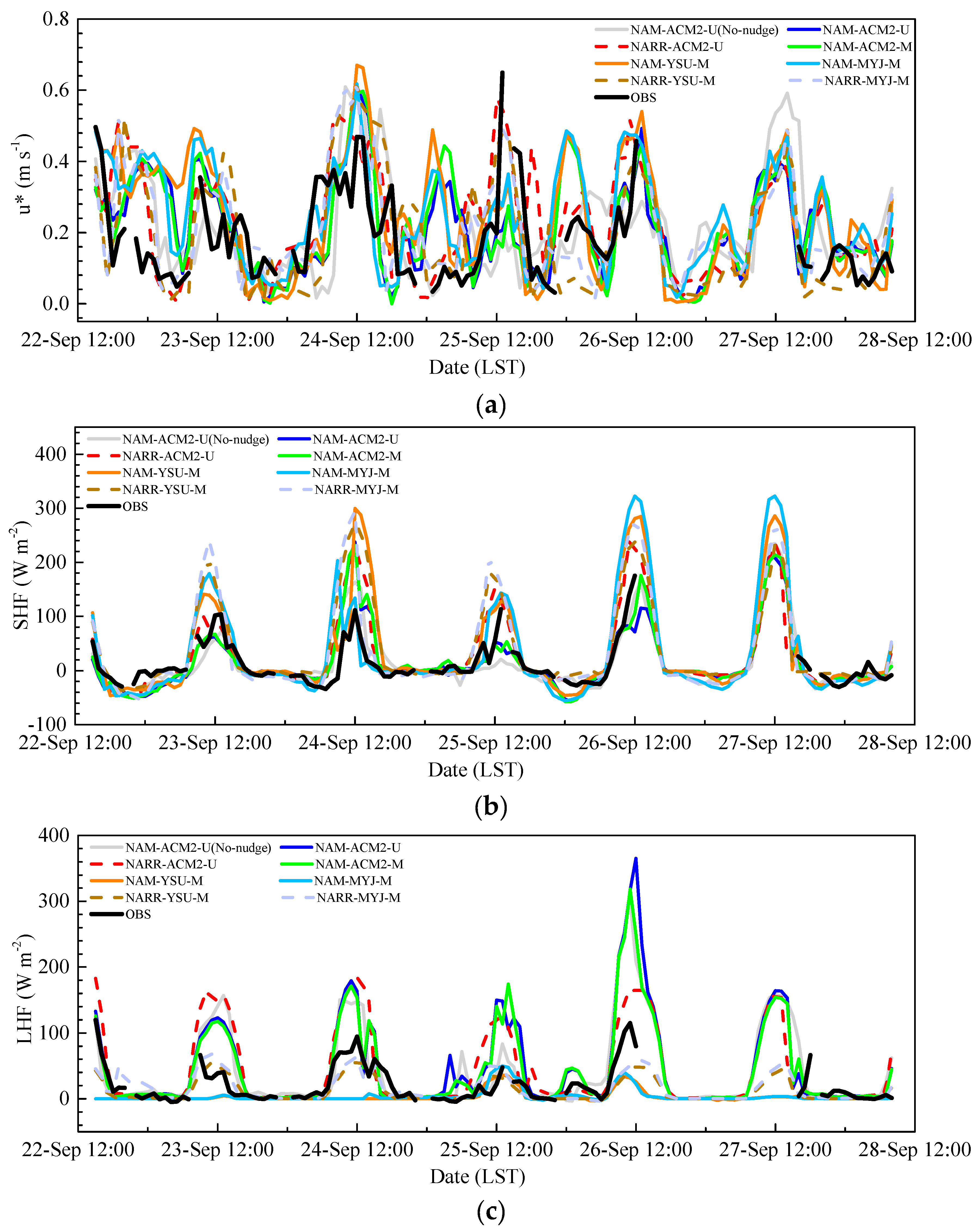
Figure 4.
Averaged simulated (a) daytime sensible heat flux, (b) nighttime sensible heat flux, (c) daytime latent heat flux, and (d) nighttime latent heat flux in the second domain (4.5 km resolution) from the eight different WRF scenarios over the observation time period.
Figure 4.
Averaged simulated (a) daytime sensible heat flux, (b) nighttime sensible heat flux, (c) daytime latent heat flux, and (d) nighttime latent heat flux in the second domain (4.5 km resolution) from the eight different WRF scenarios over the observation time period.

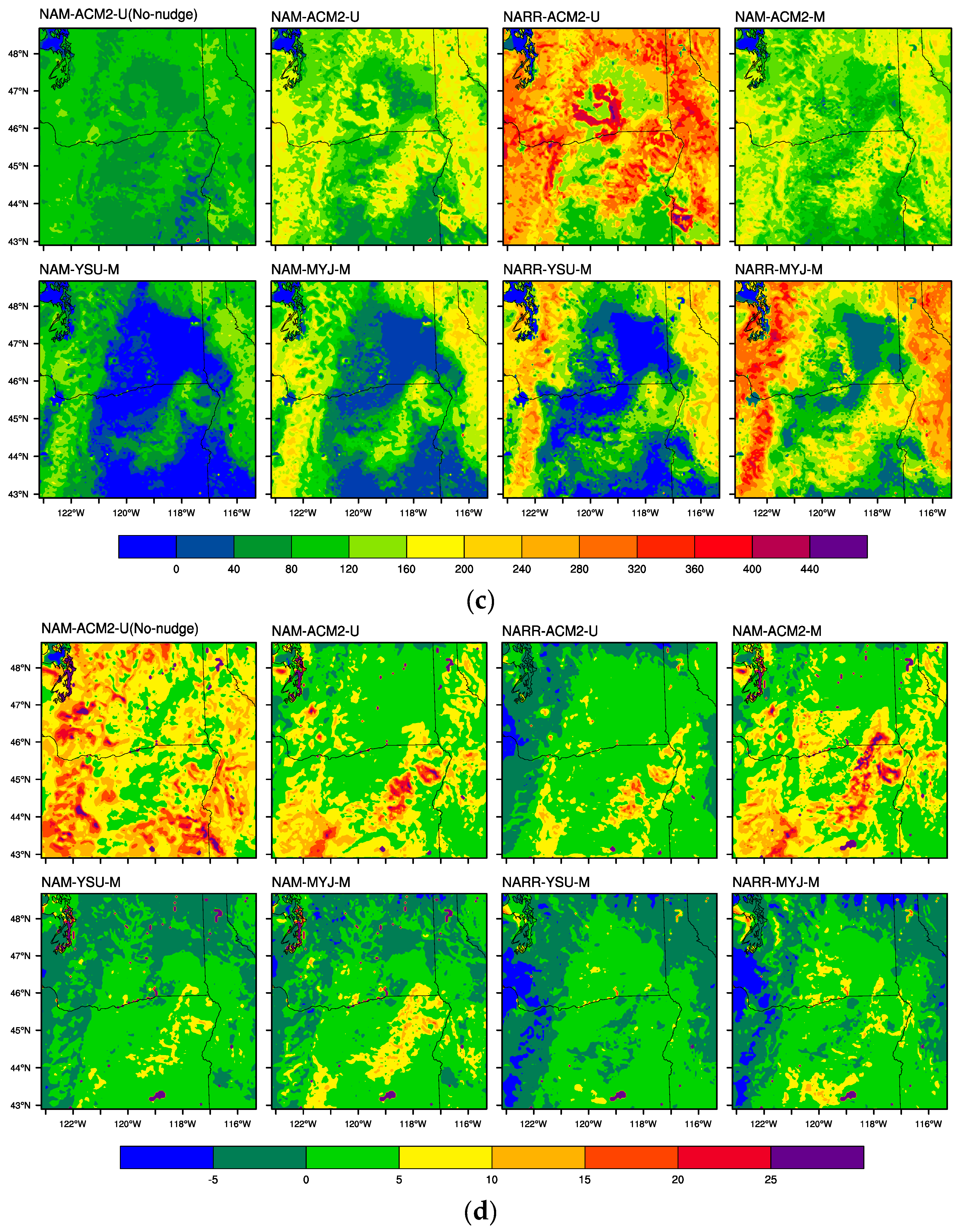
Figure 5.
Hourly time series of PBL height (Mean Sea Level, MSL) of the observation site diagnosed by the bulk Richardson number (Rib) method.
Figure 5.
Hourly time series of PBL height (Mean Sea Level, MSL) of the observation site diagnosed by the bulk Richardson number (Rib) method.

Figure 6.
WRF modeled mean vertical profiles of (a) potential temperature (theta: K) and (b) water vapor mixing ratio (q: g kg−1) at 0900, 1500, and 0300 LST over the observation site from 22 to 28 September.
Figure 6.
WRF modeled mean vertical profiles of (a) potential temperature (theta: K) and (b) water vapor mixing ratio (q: g kg−1) at 0900, 1500, and 0300 LST over the observation site from 22 to 28 September.
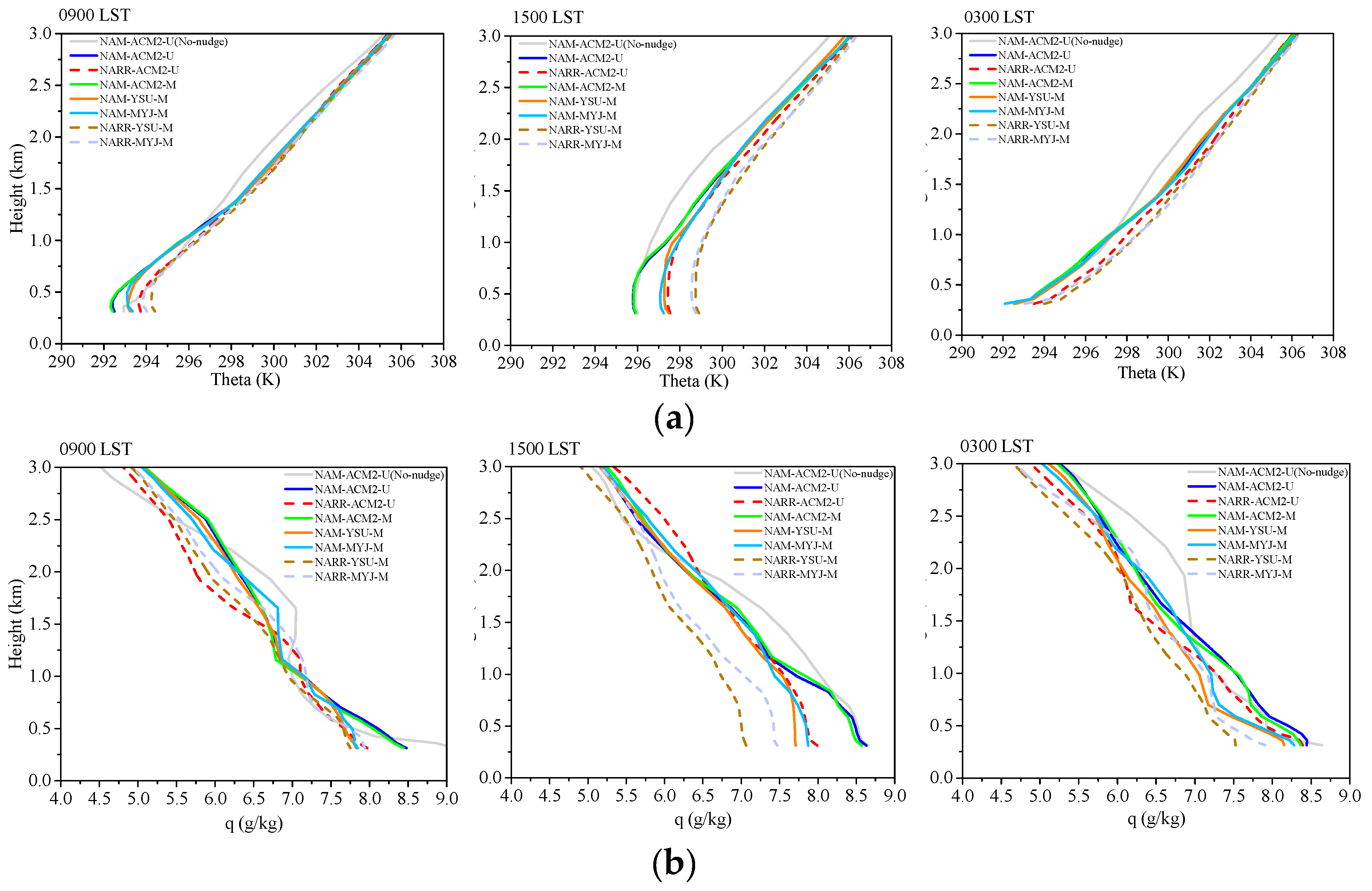
Figure 7.
Time variation of WRF simulated Rn over the flux tower site.
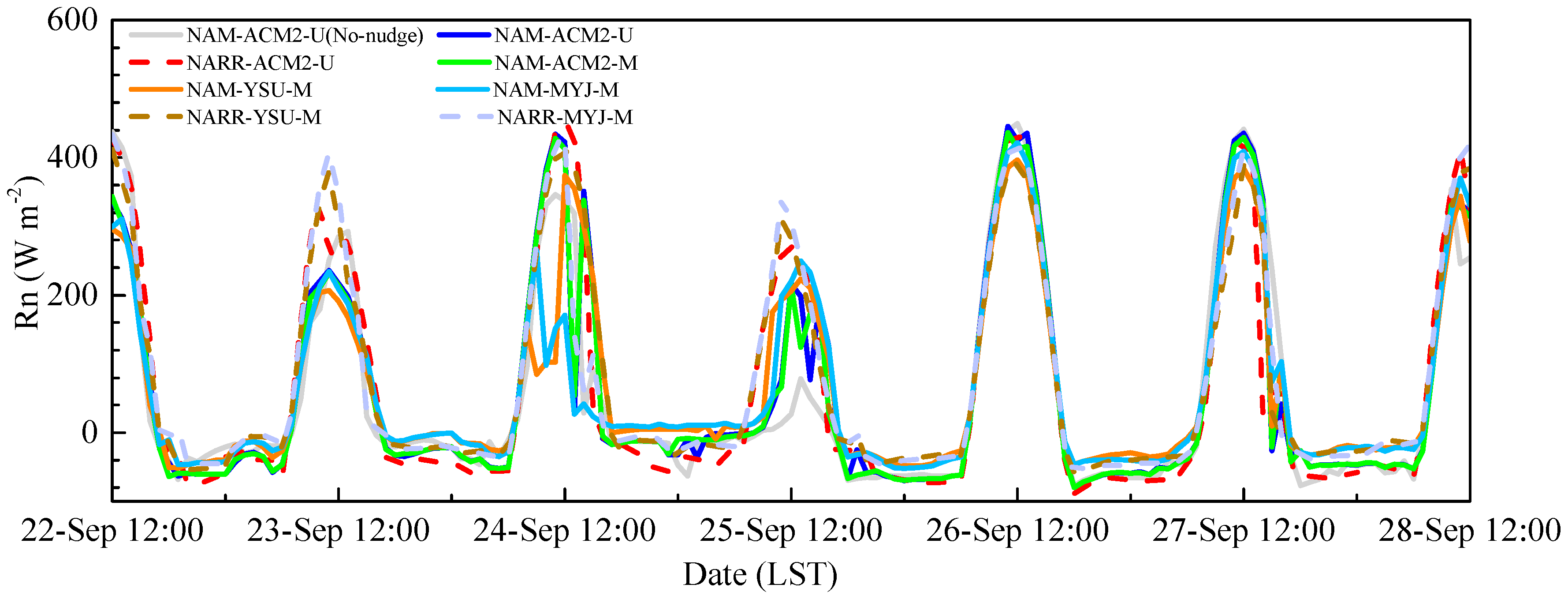
Figure 8.
Simulated (a) ground heat flux and (b) the first layer soil moisture over the observation site.
Figure 8.
Simulated (a) ground heat flux and (b) the first layer soil moisture over the observation site.

Table 1.
Summary of physics options, large-scale forcing datasets, and land-use classification datasets used in the WRF (version 3.7.1) sensitivity study.
Table 1.
Summary of physics options, large-scale forcing datasets, and land-use classification datasets used in the WRF (version 3.7.1) sensitivity study.
| Experiment | Input Forcing Data (Resolution, Interval) | Land Surface Model | Planetary Boundary Layer Scheme | Surface Layer Scheme | Land Surface INPUT Data |
|---|---|---|---|---|---|
| NAM-ACM2-U (No-nudge) | NAM (12km, 6 h) 1 | Pleim-Xiu | ACM2 2 | Pleim-Xiu Surface layer | USGS 3 |
| NAM-ACM2-U | NAM (12km, 6 h) | Pleim-Xiu | ACM2 | Pleim-Xiu Surface layer | USGS |
| NARR-ACM2-U | NARR (32km, 3 h) 4 | Pleim-Xiu | ACM2 | Pleim-Xiu Surface layer | USGS |
| NAM-ACM2-M | NAM (12 km, 6 h) | Pleim-Xiu | ACM2 | Pleim-Xiu Surface layer | MODIS 5 |
| NAM-YSU-M | NAM (12 km, 6 h) | Noah | YSU 6 | Revised MM5 Similarity | MODIS |
| NAM-MYJ-M | NAM (12 km, 6 h) | Noah | MYJ 7 | Eta similarity | MODIS |
| NARR-YSU-M | NARR (32 km, 3 h) | Noah | YSU | Revised MM5 Similarity | MODIS |
| NARR-MYJ-M | NARR (32 km, 3 h) | Noah | MYJ | Eta similarity | MODIS |
1 North American Mesoscale dataset; 2 Asymmetric Convective Model, version2; 3 U.S. Geological Survey dataset; 4 NCEP North American Regional Reanalysis dataset; 5 Moderate Resolution Imaging Spectroradiometer dataset; 6 Yonsei University boundary scheme; 7 Mellor-Yamada-Janjic boundary layer scheme.
Table 2.
Daily statistical metrics for the simulated surface meteorological variables from the eight WRF scenarios in the second domain (4.5 km horizontal resolution) using 72 surface observation locations from 22 September to 28 September 2014. Standard deviations of the metrics are included in parentheses. The lowest RMSEs are marked as bold.
| NAM- ACM2-U (No-nudge) | NAM- ACM2-U | NARR- ACM2-U | NAM- ACM2-M | NAM- YSU-M | NAM- MYJ-M | NARR- YSU-M | NARR- MYJ-M | |
|---|---|---|---|---|---|---|---|---|
| 2-m Temperature (K) | ||||||||
| MB | 0.08 (±0.59) | 0.06 (±0.35) | 0.01 (±0.33) | 0.15 (±0.38) | 0.27 (±0.18) | 0.64 (±0.16) | 0.85 (±0.21) | 1.31 (±0.18) |
| RMSE | 2.13 (±0.40) | 1.69 (±0.20) | 1.87 (±0.19) | 1.80 (±0.22) | 1.81 (±0.20) | 1.80 (±0.17) | 2.18 (±0.17) | 2.28 (±0.19) |
| IOA | 0.91 (±0.02) | 0.95 (±0.01) | 0.95 (±0.01) | 0.95 (±0.01) | 0.95 (±0.01) | 0.95 (±0.01) | 0.93 (±0.01) | 0.92 (±0.01) |
| 2-m Humidity (g kg−1) | ||||||||
| MB | 0.54 (±0.30) | 0.56 (±0.11) | 0.40 (±0.11) | 0.61 (±0.15) | 0.16 (±0.11) | 0.32 (±0.12) | −0.05 (±0.14) | 0.15 (±0.12) |
| RMSE | 1.30 (±0.25) | 0.99 (±0.12) | 0.91 (±0.14) | 1.08 (±0.13) | 0.83 (±0.14) | 0.86 (±0.11) | 0.93 (±0.14) | 0.89 (±0.09) |
| IOA | 0.75 (±0.12) | 0.87 (±0.04) | 0.88 (±0.04) | 0.84 (±0.04) | 0.90 (±0.04) | 0.90 (±0.03) | 0.87 (±0.04) | 0.88 (±0.33) |
| 10-m Wind Speed (m s−1) | ||||||||
| MB | −0.04 (±0.33) | −0.67 (±0.13) | −0.61 (±0.11) | −0.74 (±0.16) | −0.63 (±0.15) | −0.15 (±0.15) | −0.53 (±0.12) | −0.03 (±0.21) |
| RMSE | 1.80 (±0.19) | 1.56 (±0.16) | 1.61 (±0.14) | 1.64 (±0.18) | 1.59 (±0.16) | 1.60 (±0.16) | 1.75 (±0.19) | 1.87 (±0.26) |
| IOA | 0.66 (±0.07) | 0.72 (±0.06) | 0.69 (±0.06) | 0.69 (±0.07) | 0.71 (±0.06) | 0.74 (±0.06) | 0.62 (±0.08) | 0.64 (±0.09) |
| 10-m Wind Direction (deg) | ||||||||
| MB | 8.27 (±4.87) | 4.54 (±2.83) | 7.01 (±1.85) | 4.45 (±3.17) | 5.28 (±4.00) | 4.39 (±3.82) | 7.19 (±4.27) | 5.36 (±4.24) |
| RMSE | N/A1 | N/A | N/A | N/A | N/A | N/A | N/A | N/A |
| IOA | N/A | N/A | N/A | N/A | N/A | N/A | N/A | N/A |
1 N/A indicates non-available.
Table 3.
Statistics of predicted surface turbulent variables for all schemes compared with observations. Predicted values are from the domain with the finest grid resolution (0.5 km).
Table 3.
Statistics of predicted surface turbulent variables for all schemes compared with observations. Predicted values are from the domain with the finest grid resolution (0.5 km).
| Experiment | Friction Velocity (m s−1) | Sensible Heat Flux (W m−2) | Latent Heat Flux (W m−2) | ||||||
|---|---|---|---|---|---|---|---|---|---|
| RMSE1 | MB2 | MAE3 | RMSE | MB | MAE | RMSE | MB | MAE | |
| NAM-ACM2-U (No-nudge) | 0.15 | 0.03 | 0.12 | 27.51 | −3.18 | 19.03 | 46.12 | 18.15 | 26.06 |
| NAM-ACM2-U | 0.15 | 0.04 | 0.12 | 34.22 | −0.95 | 21.04 | 55.73 | 24.44 | 30.47 |
| NARR-ACM2-U | 0.14 | 0.06 | 0.11 | 38.83 | 13.25 | 22.32 | 47.88 | 23.24 | 29.52 |
| NAM-ACM2-M | 0.16 | 0.04 | 0.12 | 34.59 | −0.26 | 21.45 | 48.01 | 21.07 | 27.07 |
| NAM-YSU-M | 0.17 | 0.07 | 0.14 | 54.56 | 18.86 | 30.96 | 30.99 | −16.92 | 18.41 |
| NAM-MYJ-M | 0.16 | 0.07 | 0.12 | 49.72 | 11.45 | 29.90 | 30.54 | −15.84 | 18.08 |
| NARR-YSU-M | 0.14 | 0.02 | 0.11 | 59.25 | 27.68 | 33.61 | 20.63 | −8.53 | 13.09 |
| NARR-MYJ-M | 0.13 | 0.03 | 0.10 | 60.17 | 21.61 | 33.90 | 20.60 | −4.37 | 13.40 |
1 Root mean square error; 2 Mean bias; 3 Mean absolute error.
© 2017 by the authors. Licensee MDPI, Basel, Switzerland. This article is an open access article distributed under the terms and conditions of the Creative Commons Attribution (CC BY) license (http://creativecommons.org/licenses/by/4.0/).
Share and Cite
MDPI and ACS Style
Sun, X.; Holmes, H.A.; Osibanjo, O.O.; Sun, Y.; Ivey, C.E. Evaluation of Surface Fluxes in the WRF Model: Case Study for Farmland in Rolling Terrain. Atmosphere 2017, 8, 197. https://doi.org/10.3390/atmos8100197
AMA Style
Sun X, Holmes HA, Osibanjo OO, Sun Y, Ivey CE. Evaluation of Surface Fluxes in the WRF Model: Case Study for Farmland in Rolling Terrain. Atmosphere. 2017; 8(10):197. https://doi.org/10.3390/atmos8100197
Chicago/Turabian StyleSun, Xia, Heather A. Holmes, Olabosipo O. Osibanjo, Yun Sun, and Cesunica E. Ivey. 2017. "Evaluation of Surface Fluxes in the WRF Model: Case Study for Farmland in Rolling Terrain" Atmosphere 8, no. 10: 197. https://doi.org/10.3390/atmos8100197
Note that from the first issue of 2016, this journal uses article numbers instead of page numbers. See further details here.