The Variability of Ozone Sensitivity to Anthropogenic Emissions with Biogenic Emissions Modeled by MEGAN and BEIS3


1
Department of Environmental and Safety Engineering, Ajou University, Suwon 16499, Korea
2
Georgia Environmental Protection Division, Atlanta, GA 30354, USA
3
Air Resources Laboratory, National Oceanic and Atmospheric Administration, College Park, MD 20740, USA
4
Cooperative Institute for Climate and Satellites, University of Maryland, College Park, MD 20740, USA
*
Author to whom correspondence should be addressed.
Atmosphere 2017, 8(10), 187; https://doi.org/10.3390/atmos8100187
Submission received: 3 May 2017
/
Revised: 20 September 2017
/
Accepted: 21 September 2017
/
Published: 23 September 2017
(This article belongs to the Special Issue Tropospheric Ozone and Its Precursors)
Abstract
:In this study, we examined how modeled ozone concentrations respond to changes in anthropogenic emissions when different modeled emissions of biogenic volatile organic compounds (BVOCs) are used. With biogenic emissions estimated by the Model of Emissions of Gases and Aerosols from Nature (MEGAN) and the Biogenic Emissions Inventory System Version 3 (BEIS3), the Community Multi-scale Air Quality with the High-order Direct Decouple Method (CMAQ-HDDM) simulations were conducted to acquire sensitivity coefficients. For the case study, we chose 17–26 August 2007, when the Southern Korean peninsula experienced region-wide ozone standard exceedances. The results show that modeled local sensitivities of ozone to anthropogenic emissions in certain NOx-saturated places can differ significantly depending on the method used to estimate BVOC emission, with an opposite trend of ozone changes alongside NOx reductions often shown in model runs using MEGAN and BEIS3. Findings of increased ozone concentrations with one model and decreased ozone concentrations with the other model implies that estimating BVOCs emissions is an important element in predicting variability in ozone concentration and determining the responses of ozone concentrations to emission changes, a discovery that may lead to different policy decisions related to air quality improvement. Quantitatively, areas in the 3-km modeling domain that experienced daily maximum one-hour ozone concentrations greater than 120 ppb (MDA1O3) showed differences of over 20 ppb in MDA1O3 values between model runs with MEGAN and BEIS3. For selected monitoring sites, the maximum difference in relative daily maximum eight-hour ozone concentrations (MDA8O3) response between the methods to model BVOCs was 4.2 ppb in MDA8O3 when we adopted a method similar to the Relative Reduction Factor used by the US Environmental Protection Agency (EPA).
1. Introduction
Ozone, a persistent and prevalent urban air pollutant, imposes significant health burdens around the world, including respiratory diseases [1,2,3]. According to the World Health Organization [4], a 10 µg/m3 increment in maximum daily eight-hour ozone concentrations (MDA8O3) can increase the relative risk of mortality by 0.3%. Due to ozone’s significant adverse health effects, the South Korean government has established Ozone Air Quality Standards (O3AQS) of 0.1 ppm based on one hour of exposure and 0.06 ppm based on eight hours of exposure [5]. The government has subsequently implemented various control strategies, but many places in South Korea still experience ozone concentrations above the O3AQS.
Ground-level ozone is the product of a photochemical reaction of two major precursor species, nitrogen oxides (NOx) and volatile organic compounds (VOCs) [6,7]. Among these precursors, biogenic VOC species, including isoprene, the most abundant biogenic VOC species, have significant impacts on ozone formation because they are photochemically reactive [8,9,10].
Ozone control is difficult because (1) some precursor-emitting sources are practically uncontrollable, such as biogenic sources, and (2) these uncontrollable emissions make non-linear contributions to ozone chemistry. For this reason, quantifying the extent of ozone changes due to human intervention often requires computerized mathematical models [11,12]. These models use a range of information, including precursor emissions estimated using sub-models such as biogenic emission models, which account for various environmental conditions such as sunlight and ambient temperatures [13]. Subsequently, developing effective ozone control in an area often requires the use of a modeling system that can simulate the characteristics of ozone chemistry and precursor emissions; thus, the manner in which biogenic VOCs (e.g., isoprene) emissions are estimated will influence the results of ozone simulation, and in turn, the design of ozone control strategies.
Two biogenic emission models commonly used in practice are the Model of Emissions of Gases and Aerosols from Nature (MEGAN) and the Biogenic Emissions Inventory System Version 3 (BEIS3) [14,15,16]. In Northeast Asia, which includes South Korea, BEIS3 is rarely used because it relies on the Biogenic Emissions Land Cover Database Version 3, which is only available for the North American region. Thus, many studies in Northeast Asia have used MEGAN instead [17,18,19,20,21,22]. MEGAN often over-estimates isoprene emissions compared with BEIS3 [15,23]. According to past studies, the uncertainties in estimated isoprene emissions can be large enough to change the modeled response of ozone to reductions in anthropogenic emissions, both quantitatively and directionally [11,23,24,25]. Nevertheless, it remains unclear which model is generally the best, particularly in Northeast Asia. Even if it were not possible to accurately determine the “best” among multiple biogenic emission models, it would still be important to understand the implications of uncertainties in biogenic emissions estimates.
Thus far, proposed control strategies in South Korea have primarily focused on reducing anthropogenic precursors in non-attainment areas. According to Lee et al. [26], who used MEGAN to estimate biogenic emissions, isoprene can have a significant impact on ozone concentrations in the Seoul Metropolitan Area, South Korea, where NOx emissions are dominant. For the rest of South Korea, however, few studies regarding the sensitivity of ozone to precursor controls have considered the influence of biogenic emissions, even with one biogenic emission model. As described earlier, MEGAN may estimate higher isoprene emissions than BEIS3, and isoprene emissions can have large impacts on modeled ozone concentrations, as well as on their response to changes in precursor emissions [23].
In this study, we used the Community Multi-scale Air Quality (CMAQ) model, and compared two sets of simulated ozone concentrations and sensitivities to changes in anthropogenic emissions, using biogenic emissions estimated with MEGAN and BEIS3. For our analysis, we focused on areas that exceeded the O3AQS in and around the Southern Korean peninsula, where large cities and industrial complexes are located. For the response of ozone concentrations to changes in anthropogenic precursors, we examined absolute changes in ozone concentration as well as relative response, following an approach similar to the US EPA’s Relative Reduction Factor (RRF) method to project design values for regulatory modeling.
2. Model Period and Domains
2.1. Model Period and Domains
For this study, we ran CMAQ with a nesting-down technique. That is, the outputs of runs with a coarser grid domain were used to provide boundary conditions for runs with finer grid domains. Figure 1 shows the three CMAQ modeling domains used, which covered Northeast Asia, including China, Japan, and the Korean peninsula, along with air quality monitoring stations (AMS) and photochemical assessment monitoring stations (PAMS). AMS monitors measure criteria air pollutants (e.g., O3 and NO2), while PAMS make measurements for photochemically important VOCs (e.g., isoprene). Highly populated cities (e.g., Gwangju and Busan) and many industrial complexes (e.g., Gwangyang) are located in the Southern Korean peninsula. These areas are large sources of anthropogenic NOx and VOC emissions. In addition, the southern part of the Korean peninsula has areas of dense forest that emit large amounts of isoprene.
High-ozone days are important in our study, so we examined days in 2007 in which ozone levels exceeded the 100 ppb maximum daily one-hour ozone concentration (MDA1O3). Table 1 shows the sum of the number of days when MDA1O3 was over 100 ppb at each ozone monitor in the 3-km modeling domain. In 2007, the southern part of the Korean peninsula experienced the most monitor-days over 100 ppb during August.
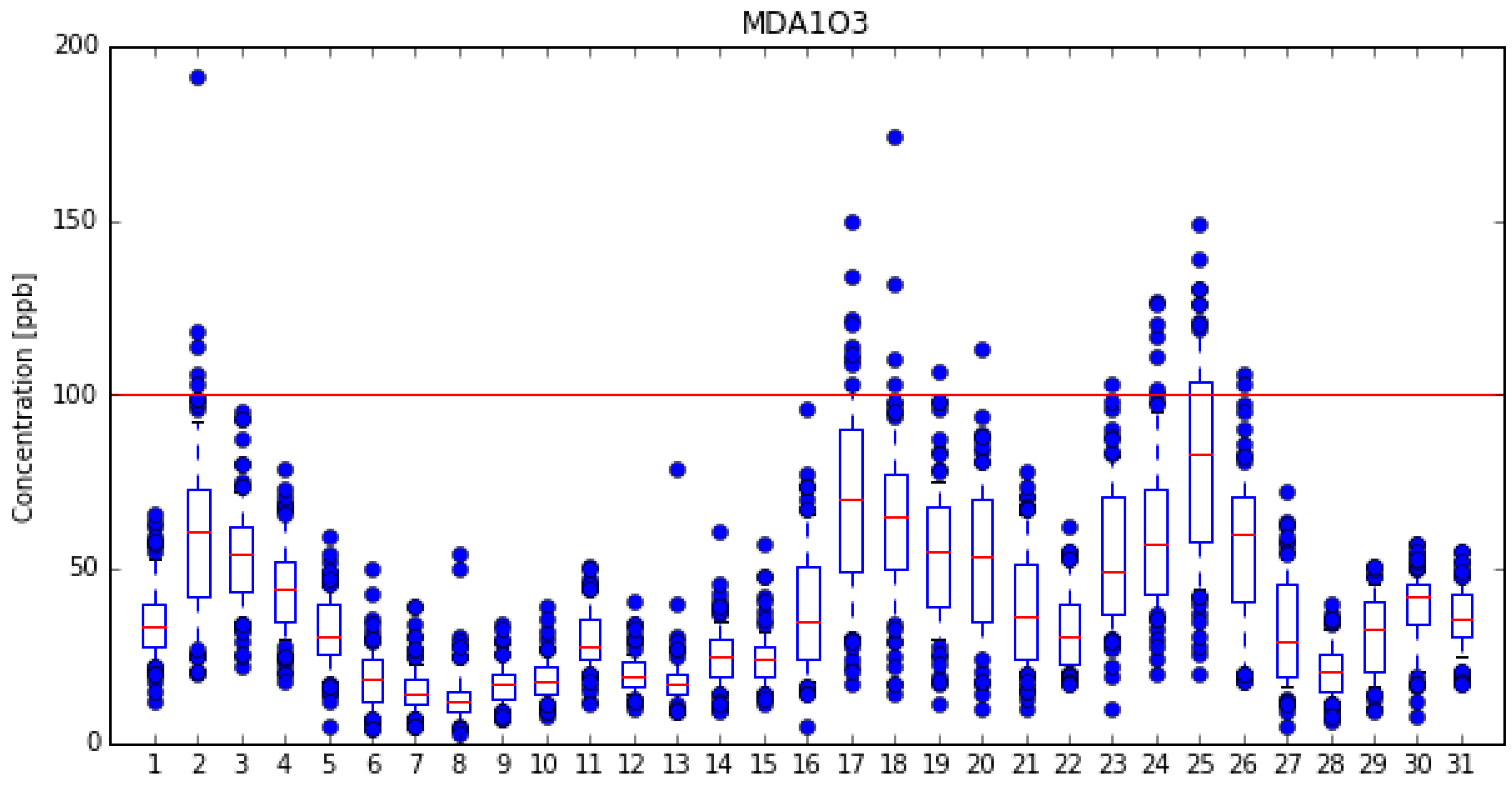
We then examined day-by-day variation in ozone concentrations. Figure 2 depicts MDA1O3 values at all monitors in the 3-km modeling domain during August 2007. Even though 2 August was when the highest MDA1O3 at one monitor was recorded, the total number of stations exceeding the 100 ppb one-hour O3AQS level was significant from 17–26 August. Table S1 shows the list of times, locations, and durations of ozone alerts, which occur when ozone concentrations are over 120 ppb. After reviewing this information, we chose to simulate 14–26 August using CMAQ.
2.2. Setup of CMAQ with High-Order Direct Decouple Method (HDDM)
For the air-quality simulations, we used CMAQ version 4.7.1 instrumented with the High-Order Direct Decouple Method, or HDDM [27,28]. According to Cohan et al. [29], modeled ozone concentrations with perturbed NOx (N) and VOCs (V) emissions, , can be approximated using the first-, second-, and cross-term sensitivity coefficients for precursors,, , , , and as follows:
where:
- is the modeled ozone concentration with perturbed NOx (N) and VOCs (V) emissions;
- is the modeled ozone concentration with no perturbation;
- is the ratio of emission changes to the original emissions;
- and are emissions before and after perturbation;
- The subscript j denotes either NOx or VOCs.
As demonstrated by Hakami [30] and Kim [31], HDDM calculates sensitivity coefficients much more efficiently than a brute-force method that requires at least two model runs for one emissions sensitivity test. In addition, HDDM accounts for the mutual impacts of changes in anthropogenic NOx and VOCs through the cross-term, . HDDM-estimated sensitivity coefficients should be quite accurate up to 90% reduction of the precursor control scenarios [32].
As defined in Equations (2) and (3), the first and second order sensitivity coefficients present degrees of ozone concentration changes and rates of those degrees due to precursor emission changes. Since various photochemical reaction environments lead to different initiation, propagation, and termination efficiency for radicals, these sensitivity coefficients are subject to change under different photochemical conditions [33]. Therefore, even though total NOx emissions and anthropogenic VOC emissions are the same, we can expect that ozone responses to anthropogenic precursor changes will be variable if different biogenic emissions are used in simulations.
2.3. Model Inputs
For meteorological inputs, Weather Research and Forecast (WRF) version 3.2 was used [34]. Final analysis (FNL) datasets from the National Center for Environmental Prediction were used to initialize the WRF run [35]. For elevation data, 90-m resolution digital elevation model data acquired from the Shuttle Radar Topography Mission were used [36]. For land-use/land-cover data, 30-s data from the United States Geological Survey (https://lta.cr.usgs.gov/GTOPO30) were used for most parts of the modeling domain, while one-second data from the Korea Ministry of Environment (https://egis.me.go.kr/intro/land.do) were used for South Korean land cells. We configured the WRF for this study as shown in Table S2. WRF outputs were processed with the Meteorology-Chemistry Interface Processor (MCIP) to feed meteorological variables into emissions processing and CMAQ runs [37].
For anthropogenic emission inputs, we used the International Chemical Transport Experiment–Phase B 2006 (INTEX-B 2006) for foreign sources [38] and the Clean Air Protection Supporting System 2007 for domestic sources [39]. These emissions were processed through the Sparse Matrix Operator Kernel Emission version 2.1 [40], with various profiles for speciation, temporalization, and spatial distribution at each source-classification code level. We used MEGAN (v2.04) and BEIS3 (v3.1) for biogenic emissions. For MEGAN, the model’s default database covering global vegetation was used. By design, BEIS3 requires Biogenic Emissions Landuse Database, Version 3 (BELD3) for its vegetation database input [41]. Since BELD3 is only available for North American regions, we had to develop BELD3-like input data for this study. For the BEIS3 run in this study, South Korea’s domestic vegetation data and emissions factors provided in the work by Cho et al. [42] were used, and we adopted the method proposed by Kim et al. [43]. Cho et al. [42] used a digitized forest-type map that contains 11 plant types and derived isoprene emission factors for each type. Kim et al. [43] updated the dataset with previous studies [44,45] to estimate biogenic emissions using BEIS3. The normalized emission rates under standard conditions (i.e., 30 °C and 1000 µmol m−2 s−1 of photosynthetically-active radiation) were adjusted with correction factors derived from hourly meteorological data from WRF to reflect meteorological variations in the model simulation, following the approach used by Pierce et al. [46]. Operational adjustment was done because, as we discuss in more detail in supplementary material Appendix A1, light correction factors can be one of the possible reasons to explain differences in emissions estimates between BEIS3 and MEGAN. For the chemical mechanism, we used Statewide Air Pollution Research Center–Version 1999 (SAPRC99) [47]. Meteorological variables processed with MCIP were used to allocate emissions vertically, if necessary.
3. Results and Discussion
3.1. Meteorological Model Performance
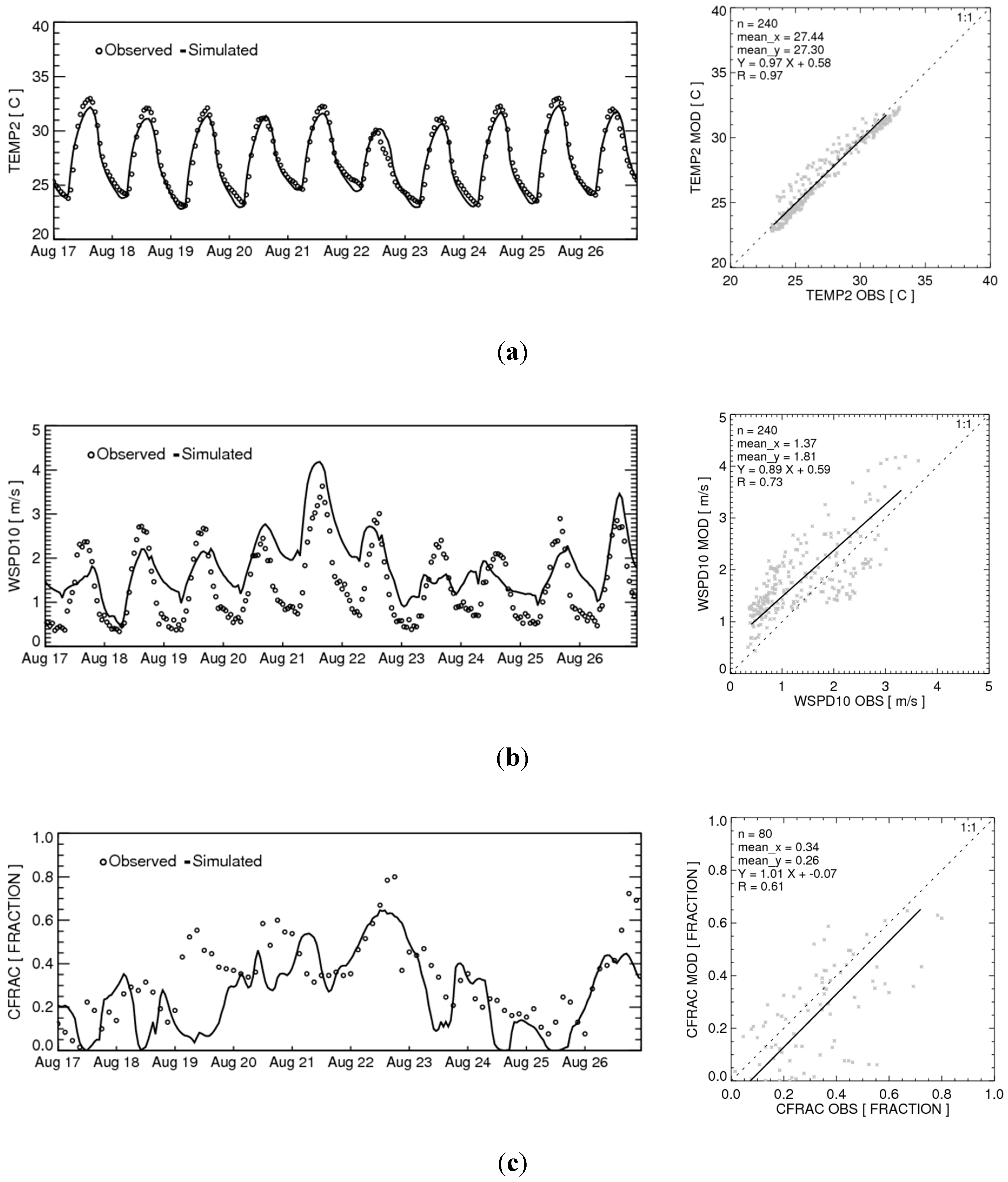
Since biogenic emissions are very sensitive to temperature and solar radiation (specifically, photosynthetical active radiation), we compared observed values of key meteorological variables with modeled values (Table S3 and Figure 3). For the comparison, we extracted modeling results at model cells where monitors are located. For the study period, WRF simulated 2-m temperatures and cloud fractions reasonably; biases of spatial averaged 2-m temperature and cloud fractions were −0.13 °C and –0.07. At hourly levels, modeled 2-m temperatures were in very good agreement with observations throughout the modeling period. Modeled 10-m wind speeds tended to show slight overprediction. During nighttime, the wind speed overprediction tendency was larger than during daytime. On 21 August, WRF grossly overpredicted 10-m wind speeds throughout the day. That may explain the slight underprediction of maximum ozone concentrations. However, this is also the day that showed the lowest ozone concentrations during the modeling period. Therefore, we believe the impact of wind speed overprediction should not be significant. For cloud fractions, only three-hour interval data were available from the observation sites. Overall, modeled cloud fractions were in very good agreement with observations, with the exception of 19, 20, and 26 August during daytime, when cloud fractions were underestimated. Notwithstanding these low cloud fraction biases, modeled ozone concentrations were not underestimated significantly. This may indicate that these days were not susceptible to biogenic emission uncertainties resulting from solar radiation biases.
3.2. Emissions and CMAQ Model Performance
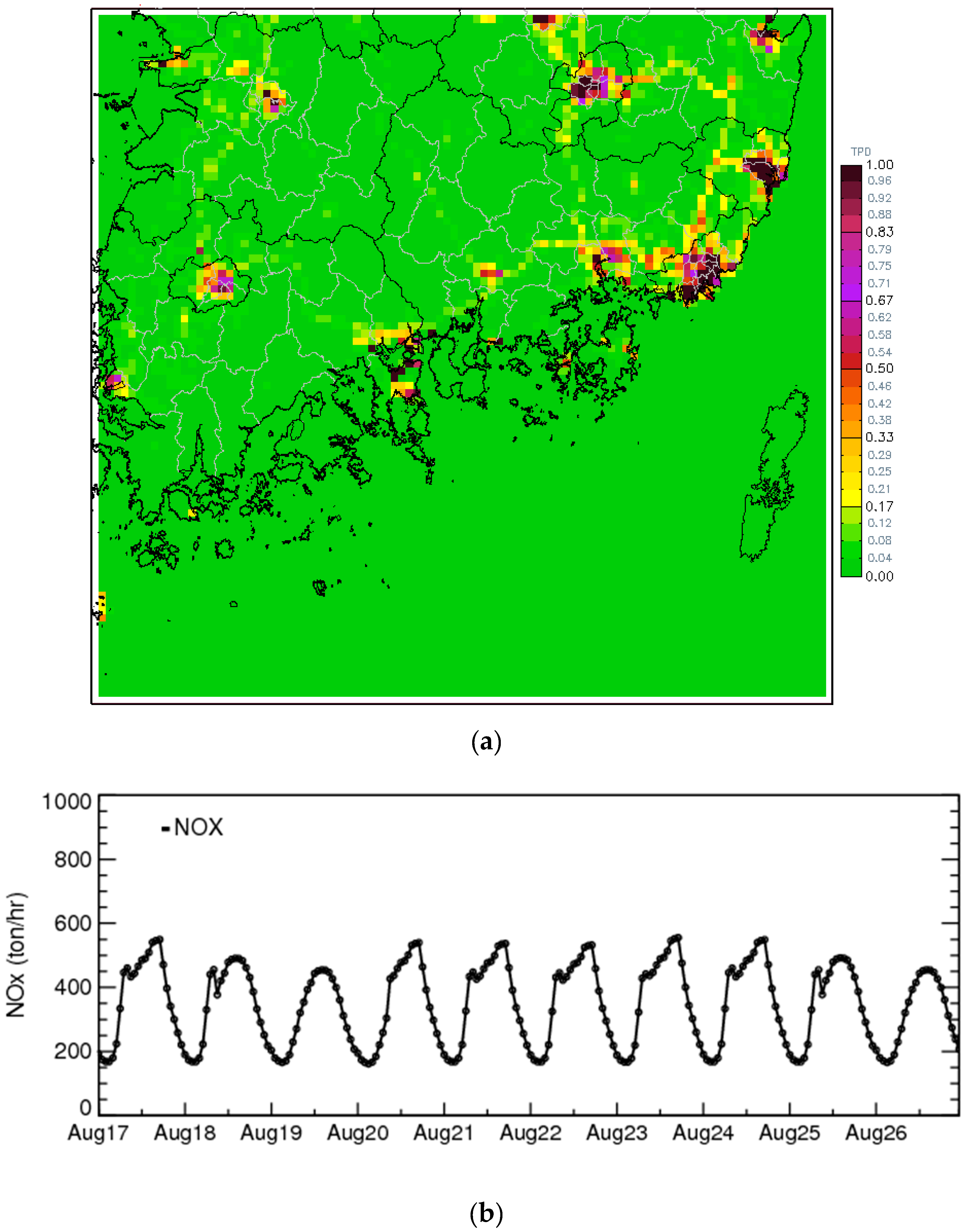
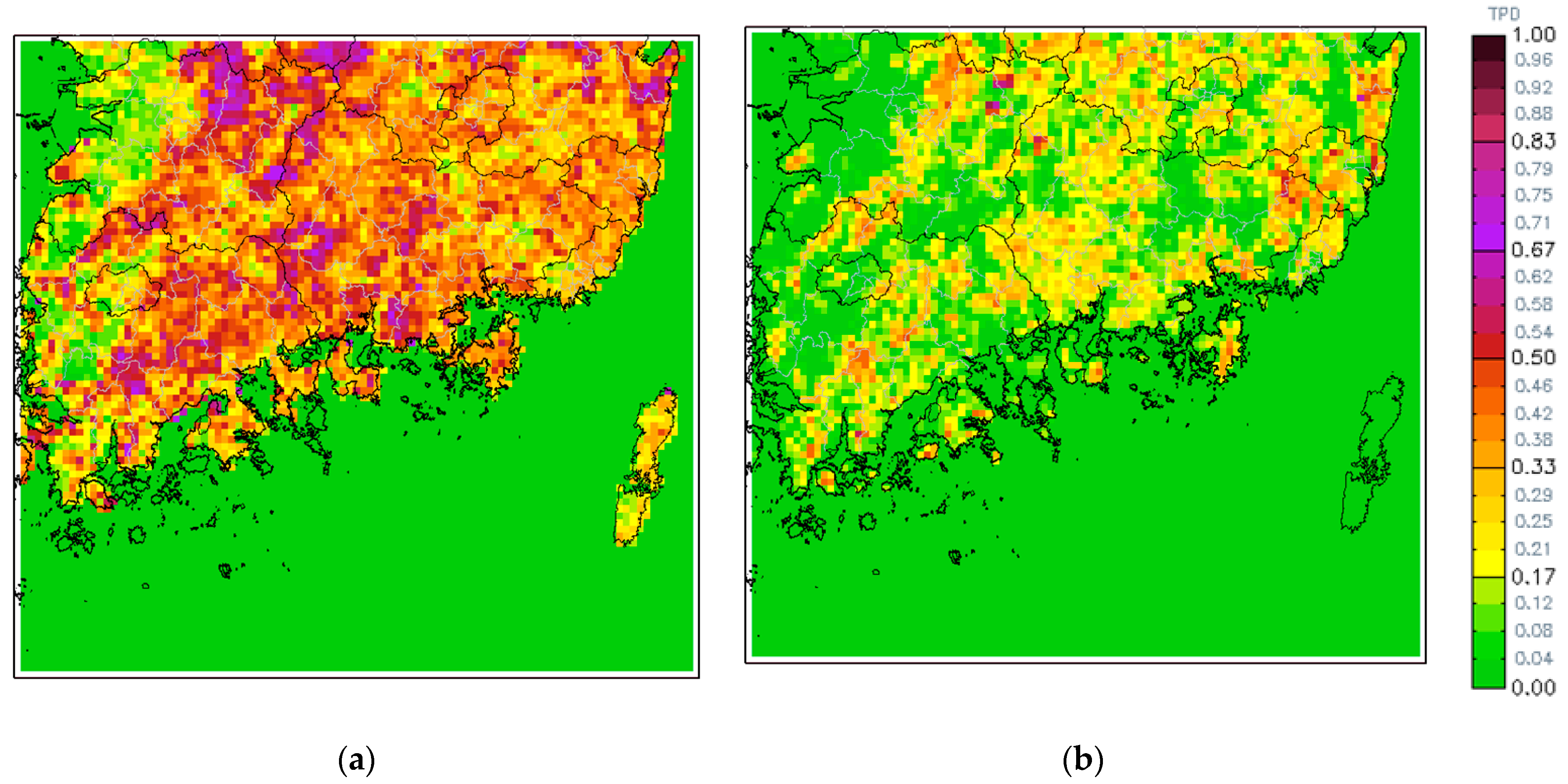
As introduced in previous sections, among the biogenic VOCs, isoprene reacts rapidly with hydroxyl radicals in the atmosphere, thereby significantly contributing to ozone concentrations [48]. For our study period, MEGAN estimated 1602 tons per day (TPD) of isoprene emissions, about 2.5 times those of BEIS3. Temporal and spatial variation of NOx emissions (Figure 4) showed typical mobile source-driven urban NOx emission profiles, which reflects the fact that most of the NOx in the study area comes from mobile sources, in general. Spatial distribution of isoprene emissions seems to be similar between the two models, qualitatively, except in low emission areas with BEIS where MEGAN shows much higher emission, relatively (Figure 5). In the United States, a similar pattern that led to gross overestimation of isoprene concentrations was reported for MEGAN, while BEIS3 had much less overestimation [49,50].
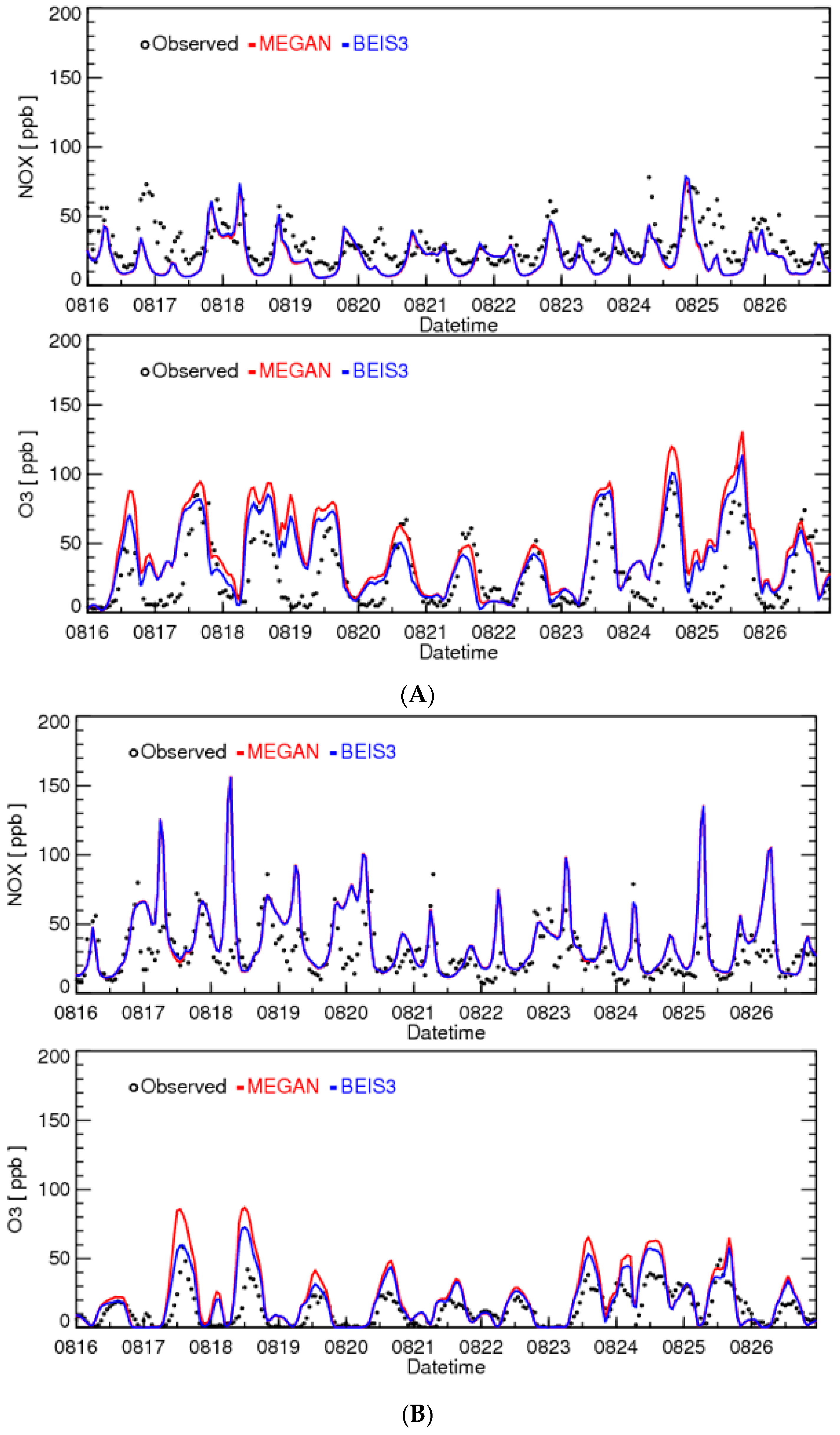
For this study period, we observed that CMAQ generally overestimated ground isoprene concentrations at PAM sites. We noted CMAQ-MEGAN had larger overestimation than did CMAQ-BEIS3 (Figure 6). Since three PAMS sites—the Daeyeon, Danggam, and Jangjun monitors—are near Busan (see Figure S1), which is the second-largest metropolitan area in South Korea, these can be susceptible to urban photochemistry. In addition, the models may not be able to achieve a good agreement with observations at these monitors because of the much greater heterogeneity of biogenic emission source distributions in urban areas. However, CMAQ at the Jeongkwan monitor showed reasonably good performance; this monitor is located near spatially homogeneous forested areas. Ultimately, it would be desirable to secure more sub-urban and rural isoprene monitors in the future. We acknowledge that the current discrepancies of isoprene concentrations between observation and model are an area for further investigation.
For NOx and O3, models show variable performance at monitors (Figure 7). Overall, CMAQ overestimated NOx regardless of the biogenic emission models used for simulations (Table S4). Similar model performance issues have been reported in many other studies [22,51,52,53,54,55,56,57,58,59,60,61]. This seems to be a systematic issue in the current modeling framework. We speculate that this is due to complex factors, such as the limitations of meteorological models (WRF in our study) in terms of vertical mixing and/or temporal profiles of NOx emissions. Further studies are warranted to reduce these types of biases. The average differences between modeled ground-level ozone and NOx concentrations due to the choice of the biogenic emissions model were about 3.54 ppb and 0.18 ppb, respectively (Table S4). Apparently, large differences in biogenic VOC emissions have very little impact on modeled ambient NO, NO2, or NOx concentrations (see Figure S2). We investigated the effects of VOC emissions on NOx further (supplementary material Appendix A1). For ozone, however, we observed that CMAQ-BEIS3 showed better model performance than CMAQ-MEGAN. Conversely, in terms of the domain-wide MDA1O3, which is often important for the purpose of regional forecasting, CMAQ-MEGAN captured the highest domain-wide daily values better than CMAQ-BEIS3. Both CMAQ-MEGAN and CMAQ-BEIS3 showed good correlations (R2 ≥ 0.8) with observed ozone. However, caution should be taken when modeling results are interpreted for longer periods because of CMAQ performance for NOx. Overpredicted NOx in the model can result in overestimated peroxyacetyl nitrate, which is thermally unstable and becomes a reservoir for additional ozone later, including the next day [62]. This characteristic can be important for prolonged stagnant conditions that can result in multiple days of high ozone concentrations. The other potential effect of overestimated NOx in the model is an underestimation of ozone concentrations near the NOx source due to titrations and then an overestimation of ozone concentrations in downwind areas when odd oxygen from ozone that is bound to NO molecules near the source during the titration process is detached as a result of NO2 photolysis and forms ozone.
3.3. Spatial Distribution of Ozone Concentrations Modeled with MEGAN and BEIS3
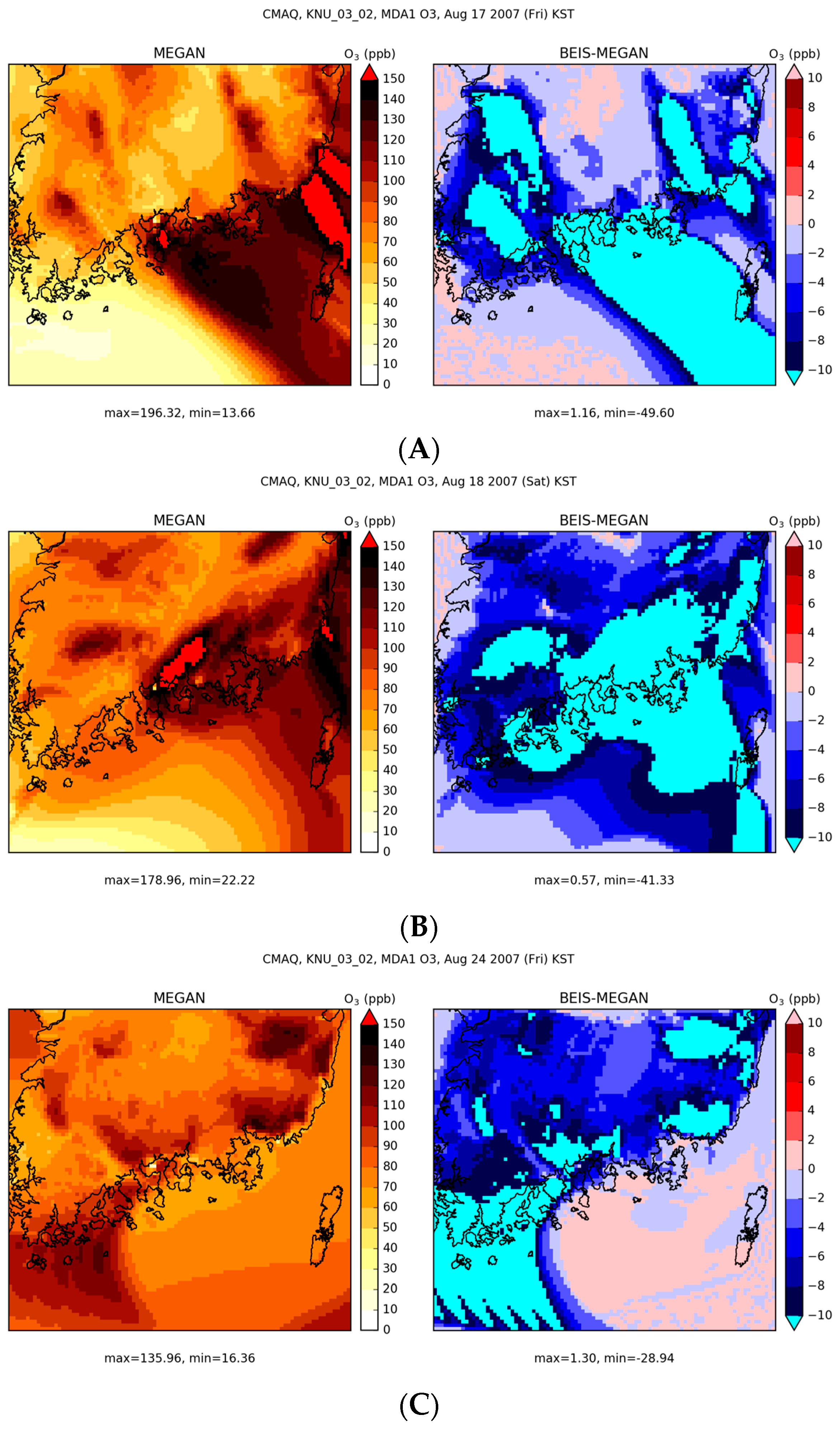
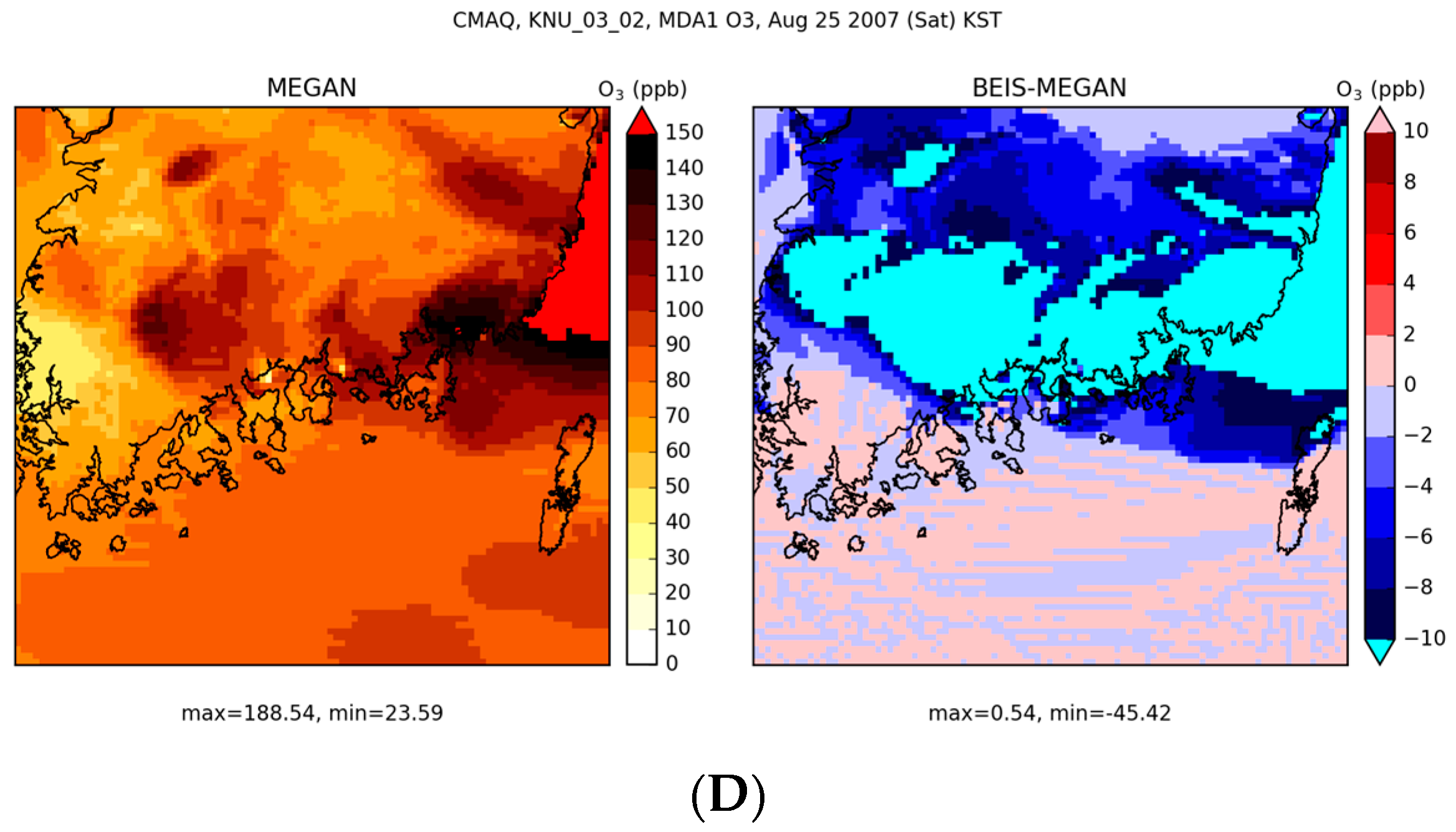
Since 17, 18, 24, and 25 August showed the highest number of ozone alerts in 2007 (Table S1), we focused spatial plots on four days when ozone concentrations in and around major cities and industrial complexes were high. Overall, CMAQ-BEIS3 estimated much lower ozone concentrations than CMAQ-MEGAN wherever high (e.g., over 120 ppb) ozone concentrations were modeled (Figure 8). In many cases where MDA1O3 was over 120 ppb, differences in modeled ozone concentrations between MEGAN and BEIS3 surpassed 20 ppb. However, these differences between CMAQ-MEGAN and CMAQ-BEIS3 should be interpreted with caution because they are not paired temporally. In other words, at a given modeling grid cell, the hour of the day corresponding to MDA1O3 predicted by CMAQ-MEGAN (e.g., 1 PM) may not be the same hour predicted by CMAQ-BEIS (e.g., 3 PM). This also brings interesting aspects when it comes to comparing daily maxima. If a plume is advected away in one model, a similar plume will move along the same path in the other model using the same meteorological field. If their photochemical evolutions do not happen at the exact same time, quite substantial concentration differences can be observed in the series of cells along the path of the plume. However, in reality, the actual difference between the two models may be very limited in its nature. This explains why there are some ripples on 24 August (Figure 8C).
Visual inspection of the hourly spatial plot series for 17, 18, 24, and 25 August 2007 revealed that high MDA1O3 values over the ocean occurred during the late night or early morning hours, and these high nighttime ozone plumes caused apparent ripples in one-hour spatial plots (Figures S3 and S4). Then, ozone was transported away from land before sunrise. Characteristics of the differences in modeled spatial distribution in ozone concentration between CMAQ-MEGAN and CMAQ-BEIS3, as shown in Figure 9, are that (1) high ozone concentrations were modeled in and around intense NOx emission sources, (2) cells with high ozone concentrations are likely to show large differences between MEGAN and BEIS3, and (3) gradients of ozone concentration differences between MEGAN and BEIS3 are steep.
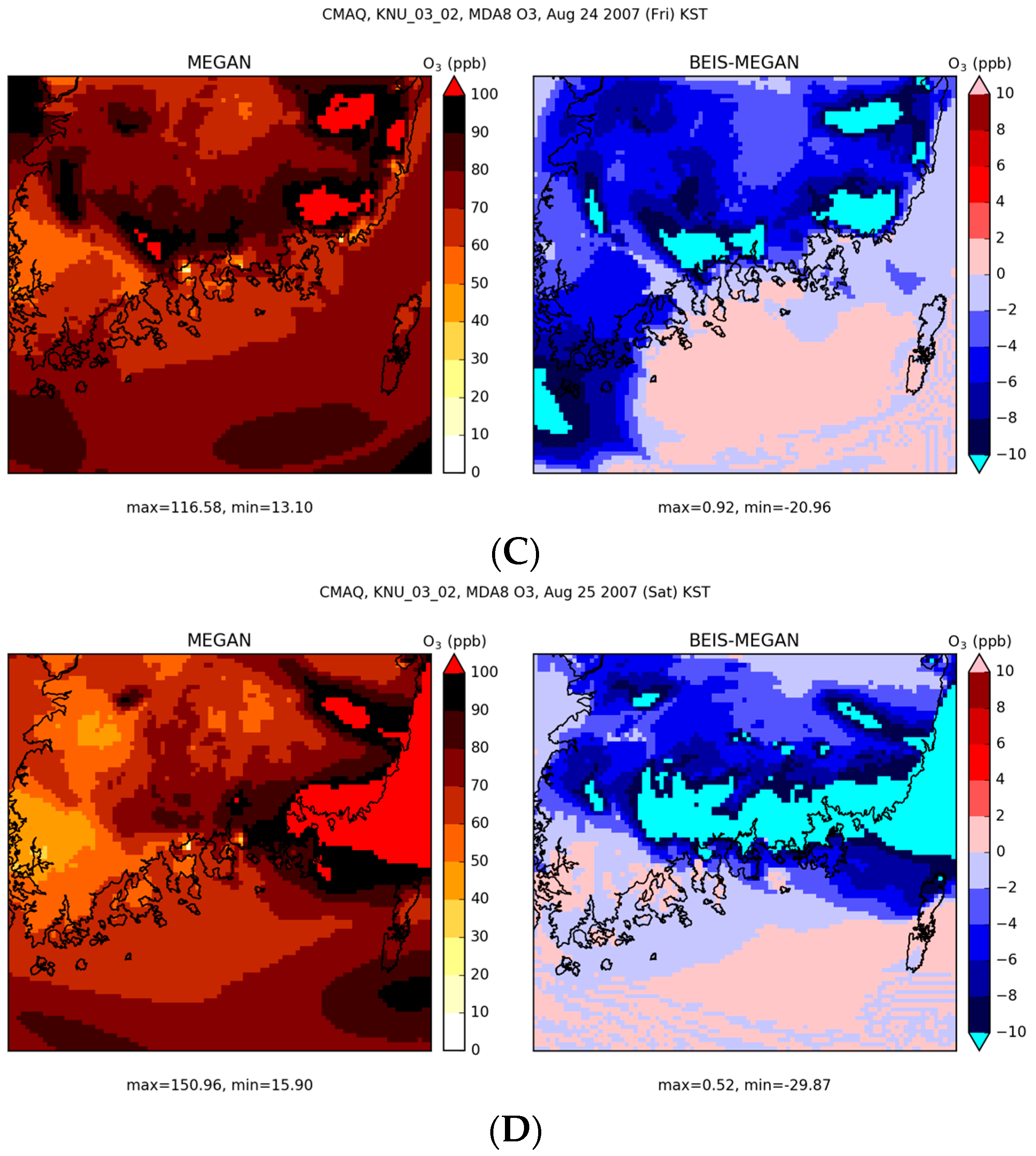
Due to the importance of health assessments (and subsequent regulatory implications), we also examined the spatial pattern of MDA8O3 (Figure 10). The overall spatial distribution of MDA8O3 and its difference between CMAQ-MEGAN and CMAQ-BEIS3 is similar to what we observed in the spatial distribution of MDA1O3, except that the ripples over the ocean were smoothed out greatly, to the extent that they seem to disappear.
3.4. Ozone Sensitivity to Anthropogenic Emissions
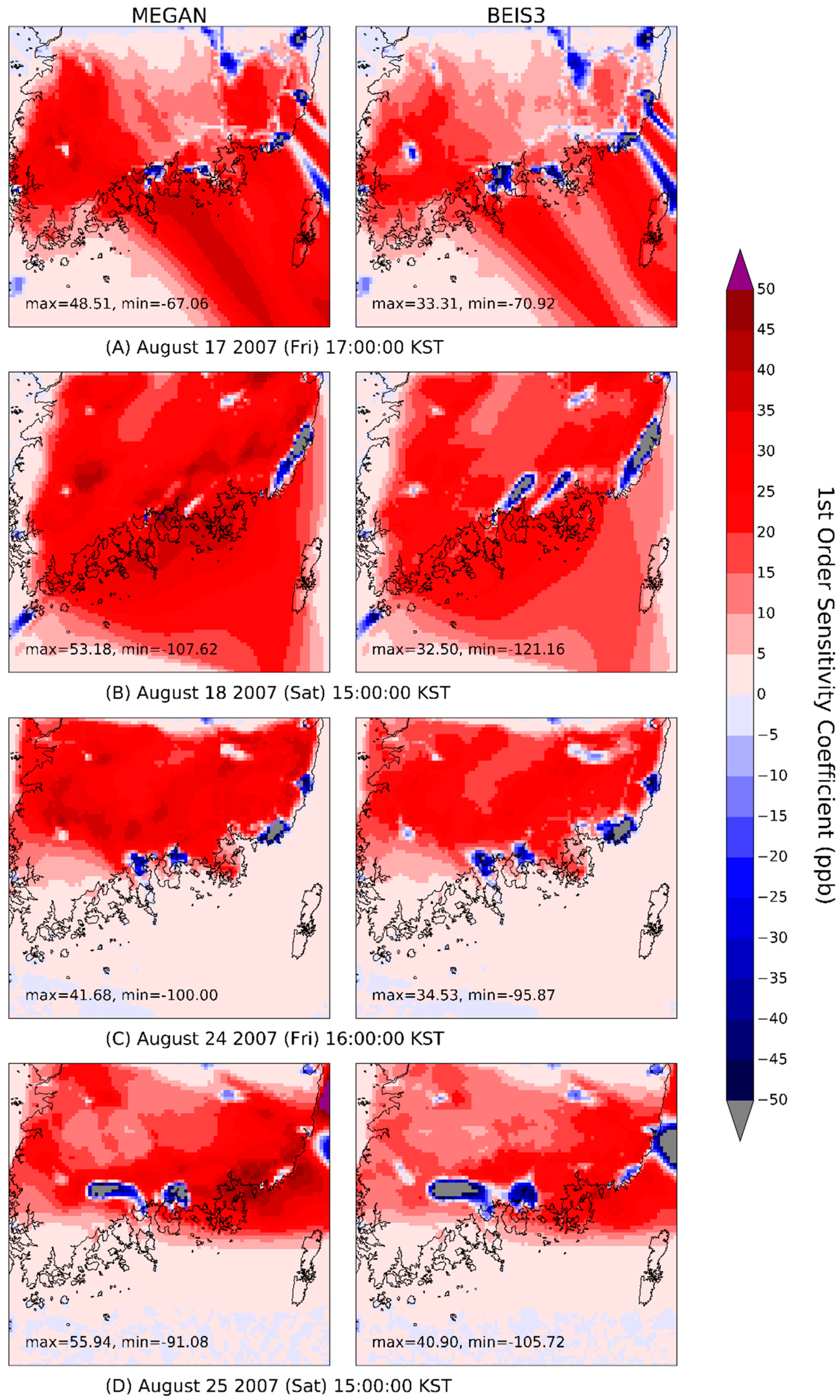
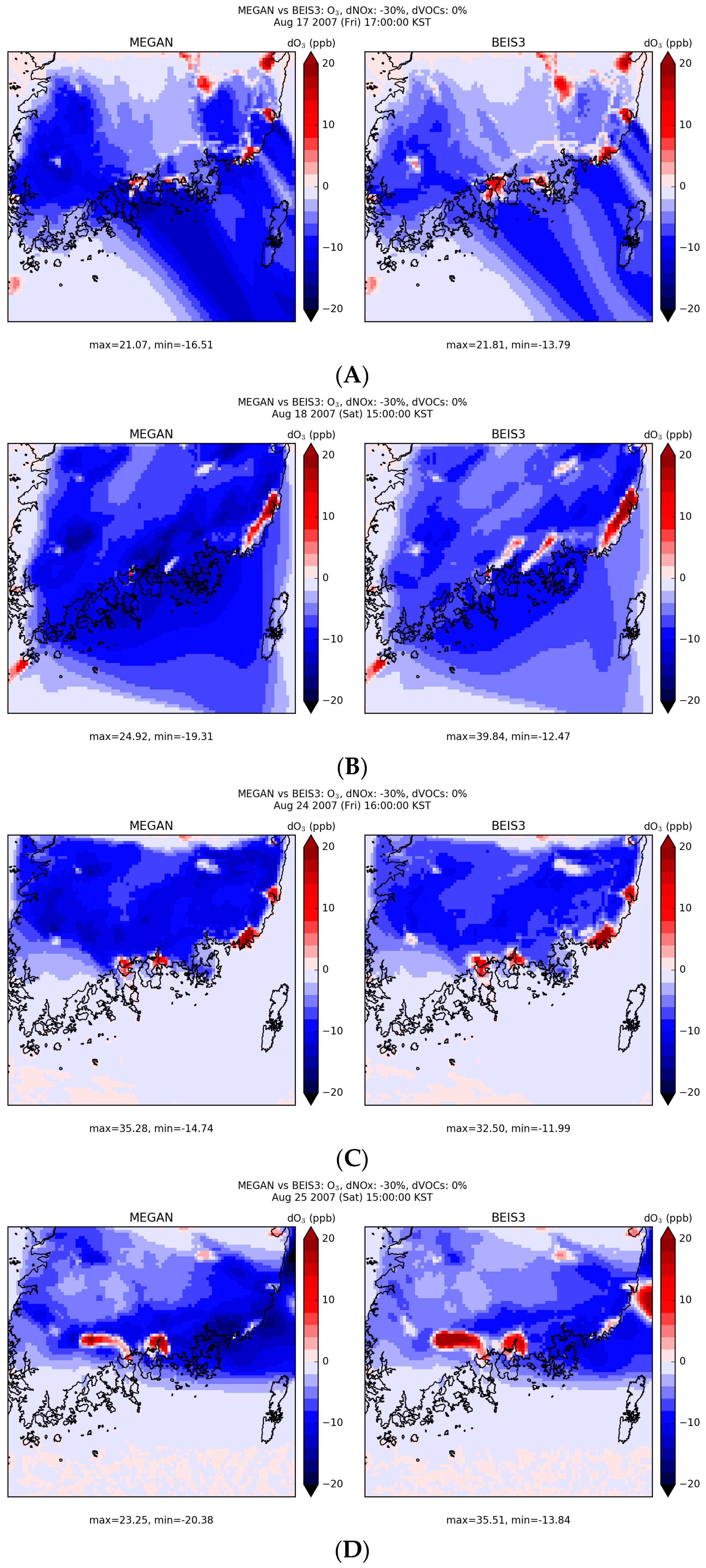
Usually, when controlling air quality, anthropogenic emissions are considered for reductions. Therefore, we examined the sensitivities of modeled ozone to reductions in anthropogenic NOx and VOCs using two different models of biogenic emissions. Figure 11 depicts the spatial distribution of the first-order sensitivity coefficients at the hours discussed in Figure 9. Figure 12 shows ozone sensitivity to 30% reductions in anthropogenic NOx at the hours of daily peak ozone concentrations on the same days. For NOx reductions, CMAQ-MEGAN and CMAQ-BEIS3 estimated similar changes in ozone for many places, but we observed significant differences in and around major cities and industrial complexes. Often, these differences between models are large enough to result in an opposite trend of changes in modeled ozone concentrations. For example, CMAQ-MEGAN estimated that a 30% reduction in anthropogenic NOx across the 3-km domain would result in a slight decrease in ozone in Gwangju at 5 PM on 17 August 2007 while CMAQ-BEIS3 estimated that the same reduction would lead to about a 5 ppb increase in ozone. Such contrasting sensitivities of ozone in high NOx emission areas were also modeled at high ozone hours on 18, 24, and 25 August 2007. These behaviors of the model, however, are not persistent throughout the modeling episode for the same locations, as they depend on the history of photochemical reactions as well as meteorological conditions, such as wind direction.
As discussed in the previous section, ozone sensitivities to reductions in anthropogenic emissions were significant in the Gwangju, Tongyoung/Geoje, Yeosu/Gwangyang, and Jinju/Sacheon areas. Gwangju is a mega-city. Tongyeong and Geoje have large manufacturing facilities, including shipyards and shipping docks. Yeosu and Gwangyang are two of the largest industrial complexes in South Korea. Jinju and Sacheon are in the downwind area of Yeosu and Gwangyang. Each of these areas represents a different emission characteristic.
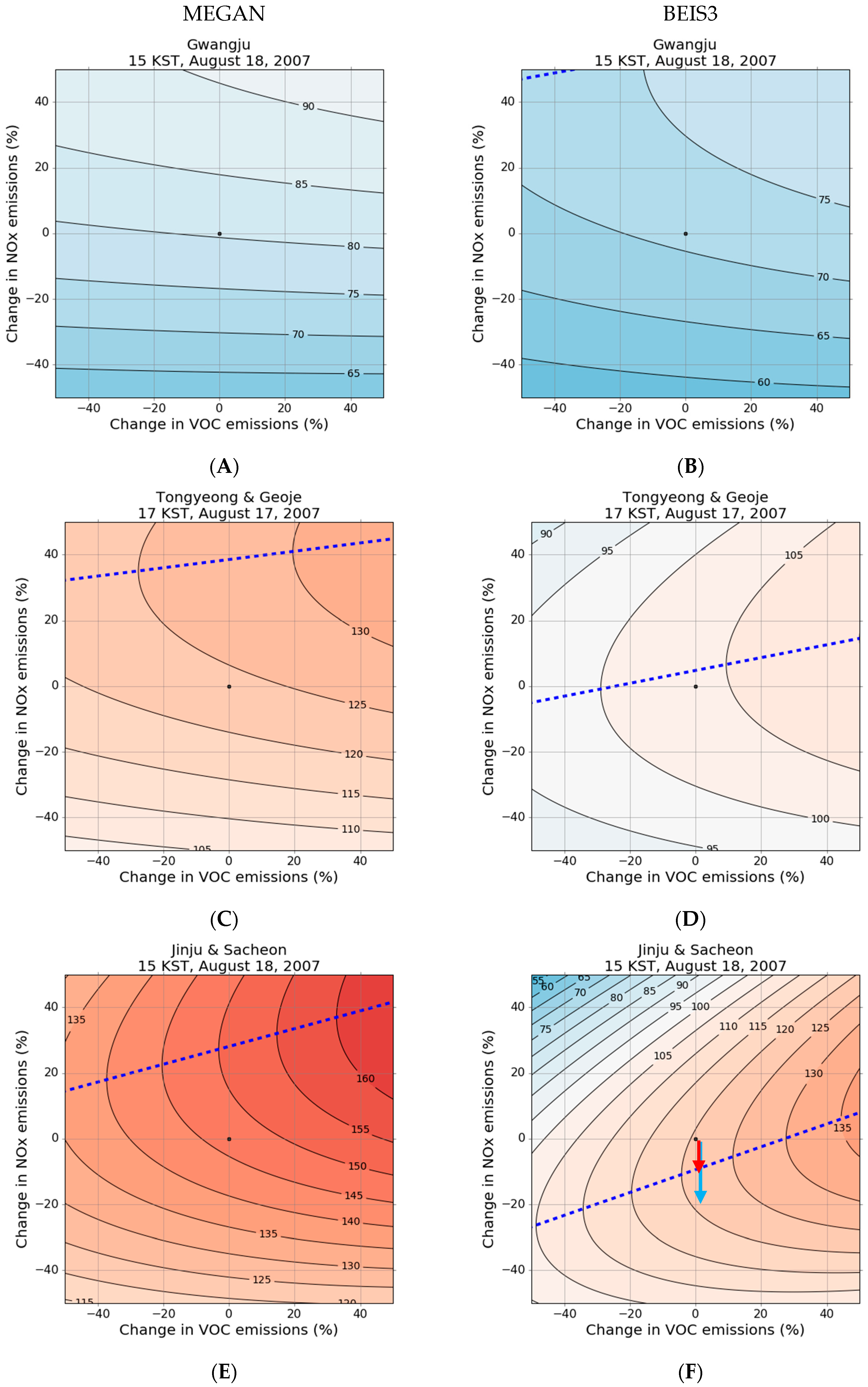
To explore ozone sensitivities in these areas over a wide range of changes in precursors when MEGAN and BEIS3 are used to estimate biogenic emissions, we examined ozone isopleths (Figure 13). We limited our isopleth analysis to ±50% of precursor emissions because the confidence of HDDM outputs may be diminished beyond 50% reductions, although results beyond 50% can still be useful [29,63]. Figure 13 contains a ridgeline for each case. A ridgeline represents a set of local maxima of ozone concentrations in the NOx-VOC space, or can be described as a set of points where ozone concentration is changing very little with NOx emission changes near it [33]. This is particularly important for air quality planning because, if the current photochemical environment is NOx-saturated (i.e., above the ridgeline), insufficient NOx control (i.e., increased NOx emissions) leads to lower ozone, or sufficient NOx control can lead to higher ozone until the ridgeline is crossed.
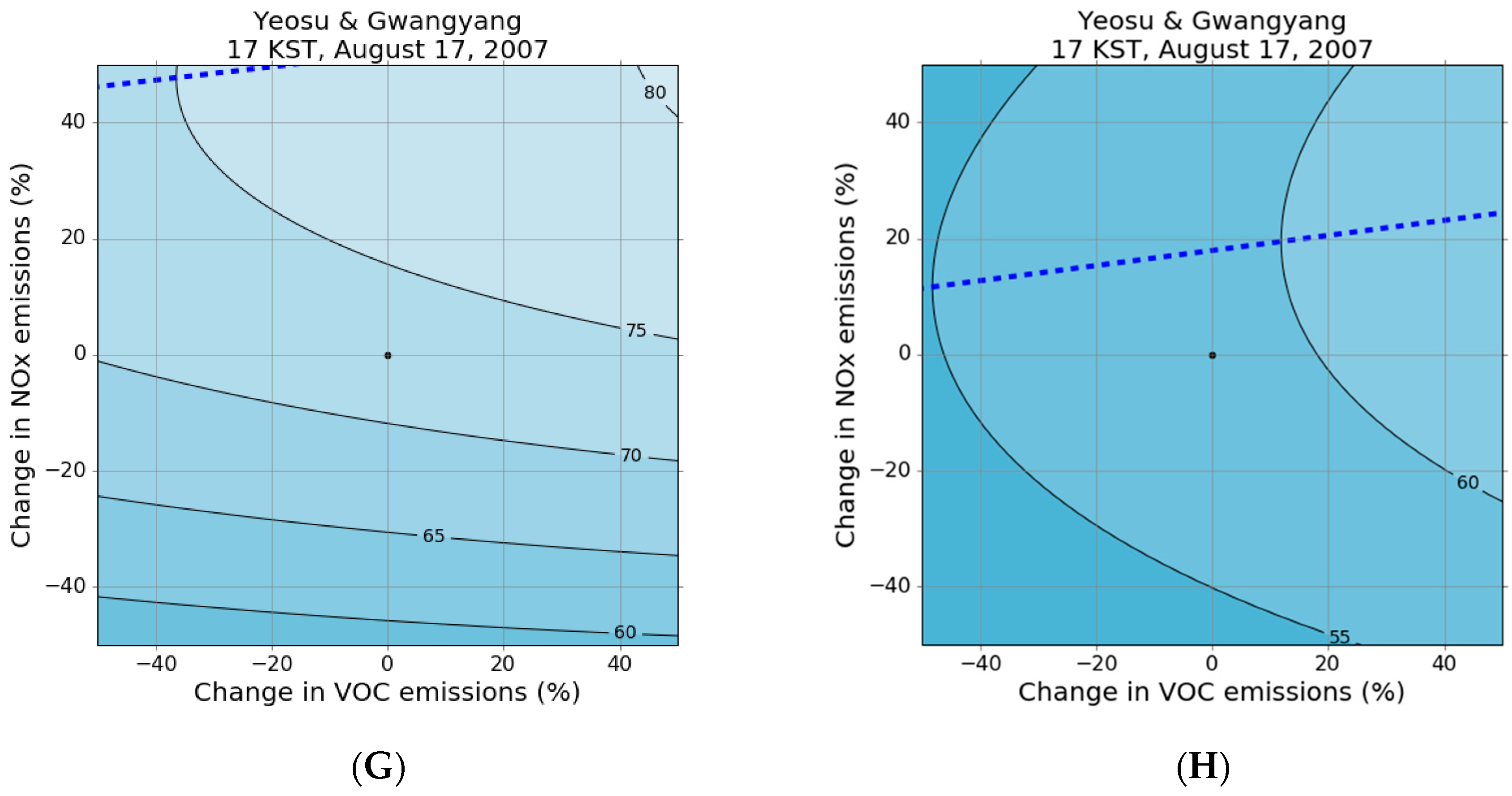
The Gwangju area (Figure 13A,B) showed differences in modeled concentrations between MEGAN and BEIS3 after reductions in anthropogenic NOx emissions, but the direction of the change was the same. In fact, both models estimated that the photochemical environment of Gwangju at 3 PM on 18 August 2017 was far away from the ridgeline. In this case, it is not likely that ozone changes due to NOx controls are qualitatively affected by the choice of biogenic emissions. The Tongyoung/Geoje (Figure 13C,D) with BEIS3 indicated that the photochemical regime of these areas at 5 PM on 17 August, 2017 was close to the ridgeline, while it was not close to the ridgeline with MEGAN. This means the simulated effects of NOx controls in this area at this hour will not show as much changes with BEIS3 as it will with MEGAN. At the same time, we can still see that the direction of changes in MEGAN and BEIS3 is the same. Notably, BEIS3 indicated that the photochemical regime of the Jinju/Sacheon (Figure 13E,F) area at 3 PM 18 August 2017 was close to but above the ridgeline, which was not the case with MEGAN. If NOx emissions were reduced by about 10% without VOC controls (following the red arrow in Figure 13F), the Jinju/Sacheon area will experience higher ozone concentrations. With a 20% reduction of NOx emissions (following the cyan color arrow in Figure 13F), the Jinju/Sacheon area will remain the same, i.e., no ozone reduction. Thus, it is obvious that the area will need not only very aggressive NOx controls but also VOC controls for visible ozone reduction results. Yeosu/Gwangyang (Figure 13G,H) had differences in both the quantities and rates of ozone change, although directional and qualitative ozone changes due to NOx controls are similar to those of Gwangju.
Photochemically speaking, the difference of ozone response between MEGAN and BEIS results from the fact that MEGAN estimates much larger biogenic emissions, which make VOCs/NOx ratios higher than BEIS3. Therefore, it has profound effects on local ozone production [64], which can be a significant source of ozone differences at downwind locations depending on airmass travel. For example, apparently, local ozone production differences in the Yeosu/Gwangyang area due to the choice of biogenic emissions were also pronounced in the Jinju and Sacheon area in the afternoon of 18 August, 2017. On isopleth plots, a net effect of higher VOCs/NOx ratios is to push the center point further right than it would be compared with BEIS3. In other words, MEGAN will likely put the base case (i.e., the origin point of isopleth plots) below a ridgeline. These behaviors have significant policy implications because they indicate the model-estimated effectiveness of NOx control can be heavily affected by biogenic emission models, even though ozone policy may focus only on anthropogenic emissions.
3.5. Ozone Concentrations Under Emissions Reduction
Environmental models are often considered to be most useful as a tool to examine sensitivities to changes in environmental conditions with respect to a baseline condition [65]. To reduce the propagation of base-year modeling uncertainties into future year (or sensitivity) modeling, the US EPA developed a procedure to use photochemical modeling results in a relative sense when such models are used for regulatory purposes [66]. In this procedure, the Relative Reduction Factor is defined as the ratio of modeled future year concentrations to modeled base year concentrations for days over a certain threshold. In our study, we observed quite large uncertainties between the two biogenic models. Therefore, adopting this idea without setting thresholds or cutoffs, we applied the RRF to our results for reductions of 30% NOx-only, 30% VOCs-only, and both 30% NOx and 30% VOCs. For this analysis, we selected monitors in the Yeosu/Gwangyang area where large differences between MEGAN and BEIS occurred: the Samil-dong, Wollae-dong, Jung-dong, and Chilsung-li monitors. For each monitor, we computed relative response factors as follows:
where I is a day modeled. Here, represents MDA8O3 values from the baseline run. represents MDA8O3 values with reductions in NOx and/or VOCs emissions.
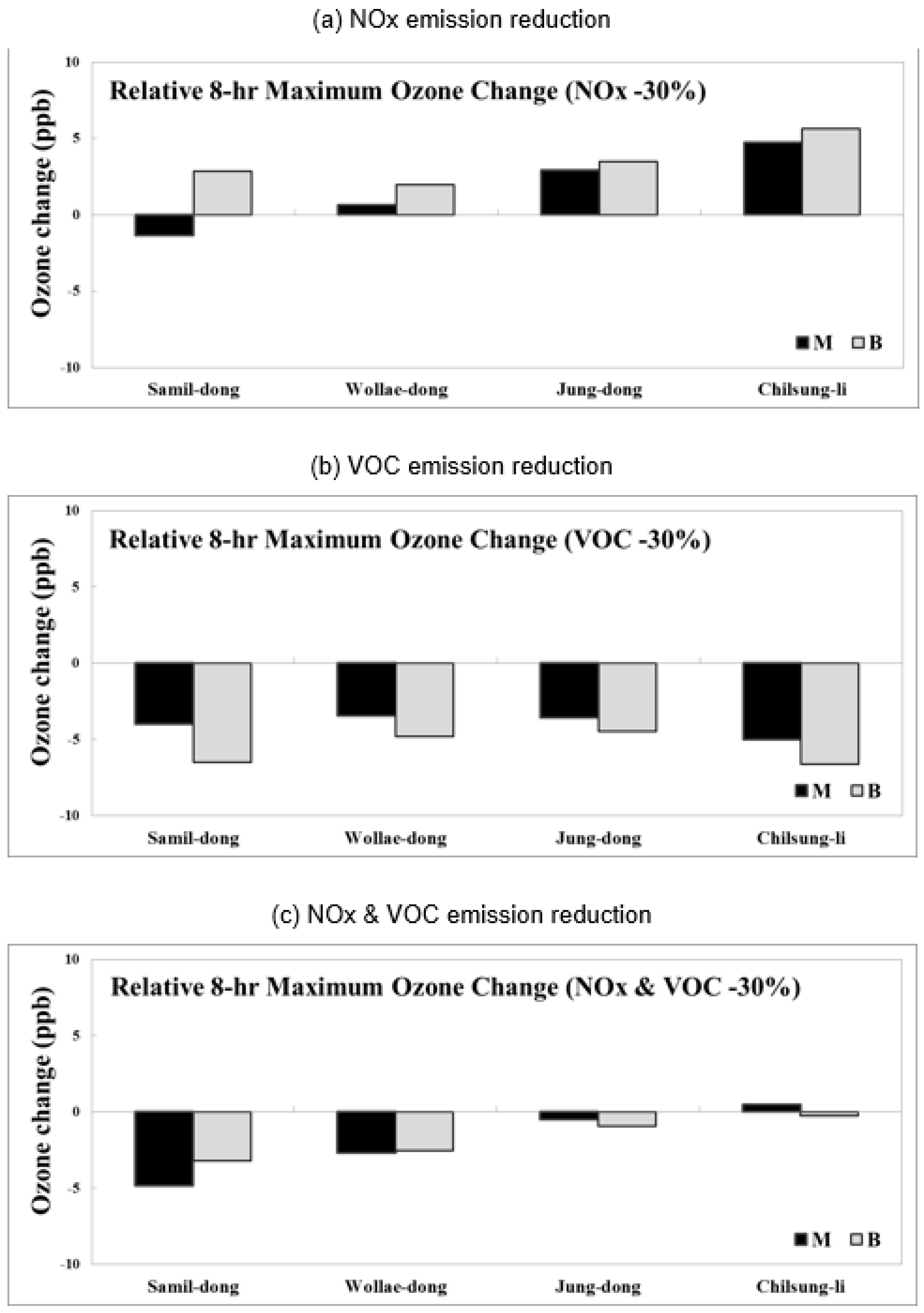
We then multiplied the RRFs by the ozone concentrations observed at these monitors. Figure 14 compares the averaged MDA8O3 values throughout the modeling period with and without the RRF application. In many cases, CMAQ-MEGAN estimated smaller changes in ozone concentration, although ozone concentrations estimated with CMAQ-MEGAN are higher than those estimated with CMAQ-BEIS3. With 30% NOx-only, 30%-VOCs only, and both 30% NOx and 30% VOCs reduction, the maximum differences among all monitors in relative ozone response were 4.2 ppb, 2.5 ppb, and 1.6 ppb, respectively. At the Samil-dong monitor with 30% NOx reduction and at the Chilsung-li monitor with both 30% NOx and VOCs reduction, modeled ozone changes estimated by CMAQ-MEGAN and CMAQ-BEIS3 had different signs. CMAQ-MEGAN results suggested that simultaneous precursor reductions could lead to greater reductions in ozone than CMAQ-BEIS3 results suggested. As we discussed in the Jinju/Sacheon area case in the previous section, ozone responses at these monitors can vary greatly depending on their modeled photochemical regimes. In addition, as our RRF analysis shows, modeling biases may amplify or shrink the effects of photochemical conditions on ozone concentrations after anthropogenic precursor emission controls are applied. We present more cases with RRF applications in the Supplementary Material (Figures S5–S8).
These results indicate that photochemical modeling for assessing ozone control scenarios in South Korea requires careful consideration of biogenic emissions, even though biogenic emissions may not be included as part of the control strategy. For sites showing opposing trends of ozone responses to precursor reductions when modeled with MEGAN or BEIS3, we recommend performing additional corroborative analyses, such as sensitivity analyses or observation-based analyses, to ensure that precursor controls will lead to the anticipated results, at least qualitatively or directionally.
4. Conclusions
We conducted CMAQ simulations to estimate ozone concentrations and the responses of these modeled concentrations to changes in precursor emissions in the southern Korean peninsula from 16–29 August 2007 using two biogenic emissions models, MEGAN and BEIS3. We utilized HDDM to obtain sensitivity coefficients, and compared the results of CMAQ-MEGAN and CMAQ-BEIS3. MEGAN estimated higher isoprene concentrations, about twice those estimated with BEIS3. This result is consistent with what has been reported in previous studies. Both CMAQ-MEGAN and CMAQ-BEIS3 slightly overestimated ozone concentrations, although CMAQ-BEIS3 showed better accuracy overall for ozone than CMAQ-MEGAN. As for domain-wide peak ozone concentrations, CMAQ-MEGAN-modeled ozone concentrations were closer to the observed values than CMAQ-BEIS3. During the modeling period across the 3-km modeling domain, differences in modeled one-hour concentration between CMAQ-MEGAN and CMAQ-BEIS3 were often over 20 ppb, especially near large cities and industrial complexes. Sensitivities to reductions in ozone precursors led CMAQ-MEGAN and CMAQ-BEIS3 to predict different directions of ozone response, an effect that is expressed much more in areas with many NOx sources, such as around large cities and industrial complexes. Due to inherited uncertainties or biases in modeled absolute concentrations, we adopted the US EPA’s RRF procedure to re-evaluate modeled ozone changes due to precursor reductions. With RRF, modeled ozone changes were smaller with CMAQ-MEGAN than with CMAQ-BEIS3. Furthermore, we observed that CMAQ-MEGAN and CMAQ-BEIS3 still estimated directionally different ozone responses under certain conditions. For example, CMAQ-MEGAN estimated a decrease in ozone concentration for 30% NOx reduction, while CMAQ-BEIS3 predicted an increase in ozone concentration for the same case. We believe this behavior implies that air quality modeling in South Korea for assessing policy scenarios requires careful consideration of biogenic emission models, as well as the incorporation of other corroborative analyses, in order to ensure the effectiveness of ozone control strategies.
Supplementary Materials
The supplementary materials are available online at https://www.mdpi.com/2073-4433/8/10/187.
Acknowledgments
This work was supported by a grant from the National Institute of Environment Research (NIER), funded by the Ministry of Environment (MOE) of the Republic of Korea (NIER-2017-01-02-045) and the South Korea Ministry of Environment (MOE) “Public Technology Program for Environmental Industry”.
Author Contributions
Eunhye Kim and Soontae Kim conceived and designed the experiments; Eunhye Kim performed the experiments; Eunhye Kim, Soontae Kim, and Byeong-Uk Kim analyzed the data; Hyun Cheol Kim and Byeong-Uk Kim contributed analysis tools; Eunhye Kim and Byeong-Uk Kim wrote the paper.
Conflicts of Interest
The authors declare no conflict of interest.
Disclaimer
The scientific results and conclusions, as well as any views or opinions expressed herein, are those of the authors and do not necessarily reflect the views of NOAA or the Department of Commerce.
References
- Cohen, A.J.; Anderson, H.R.; Ostro, B.; Pandey, K.D.; Krzyzanowski, M.; Künzli, N.; Gutschmidt, K.; Pope, C.A., III; Romieu, I.; Samet, J.M.; et al. Urban air pollution. Comp. Quantif. Health Risks 2004, 2, 1353–1433. [Google Scholar]
- Royal Society. Ground-Level Ozone in the 21st Century: Future Trends, Impacts and Policy Implications; The Royal Society: London, UK, 2008; ISBN 978-0-85403-713-1. [Google Scholar]
- U.S. EPA. Integrated Science Assessment (ISA) of Ozone and Related Photochemical Oxidants (Final Report, February 2013). Available online: https://cfpub.epa.gov/ncea/isa/recordisplay.cfm?deid=247492 (assessed on 2 February 2017).
- World Health Organization. Health Risks of Ozone from Long-range Transboundary Air Pollution. 2008. Available online: http://www.euro.who.int/__data/assets/pdf_file/0005/78647/E91843.pdf?ua=1 (assessed on 23 February 2017).
- Ministry of Environment. Air Quality Standards and Air Pollution Level. Available online: http://eng.me.go.kr/eng/web/index.do?menuId=252 (accessed on 26 February, 2017).
- Finlayson-Pitts, B.J.; Pitts, J.N., Jr. Chemistry of the Upper and Lower Atmosphere: Theory, Experiments, and Applications; Academic press: Cambridge, MA, USA, 1999. [Google Scholar]
- Seinfeld, J.H.; Pandis, S.N. Atmospheric Chemistry and Physics: From Air Pollution to Climate Change; John Wiley & Sons: Hoboken, NJ, USA, 2016. [Google Scholar]
- Fiore, A.M. Evaluating the contribution of changes in isoprene emissions to surface ozone trends over the eastern United States. J. Geophys. Res. 2005, 110. [Google Scholar] [CrossRef]
- Ito, A.; Sillman, S.; Penner, J.E. Global chemical transport model study of ozone response to changes in chemical kinetics and biogenic volatile organic compounds emissions due to increasing temperatures: Sensitivities to isoprene nitrate chemistry and grid resolution. J. Geophys. Res. 2009, 114. [Google Scholar] [CrossRef]
- Hewitt, C.N.; Ashworth, K.; Boynard, A.; Guenther, A.; Langford, B.; MacKenzie, A.R.; Misztal, P.K.; Nemitz, E.; Owen, S.M.; Possell, M.; et al. Ground-level ozone influenced by circadian control of isoprene emissions. Nat. Geosci. 2011, 4, 671–674. [Google Scholar] [CrossRef]
- Russell, A.; Dennis, R. NARSTO critical review of photochemical models and modeling. Atmos. Environ. 2000, 34, 2283–2324. [Google Scholar] [CrossRef]
- Monks, P.S.; Archibald, A.T.; Colette, A.; Cooper, O.; Coyle, M.; Derwent, R.; Fowler, D.; Granier, C.; Law, K.S.; Mills, G.E.; et al. Tropospheric ozone and its precursors from the urban to the global scale from air quality to short-lived climate forcer. Atmos. Chem. Phys. 2015, 15, 8889–8973. [Google Scholar] [CrossRef] [Green Version]
- Pugh, T.A.M.; Ashworth, K.; Wild, O.; Hewitt, C.N. Effects of the spatial resolution of climate data on estimates of biogenic isoprene emissions. Atmos. Environ. 2013, 70, 1–6. [Google Scholar] [CrossRef]
- Guenther, C.C. Estimates of global terrestrial isoprene emissions using MEGAN (Model of Emissions of Gases and Aerosols from Nature). Atmos. Chem. Phys. 2006, 6, 3181–3210. [Google Scholar] [CrossRef] [Green Version]
- Carlton, A.G.; Baker, K.R. Photochemical Modeling of the Ozark Isoprene Volcano: MEGAN, BEIS, and Their Impacts on Air Quality Predictions. Environ. Sci. Technol. 2011, 45, 4438–4445. [Google Scholar] [CrossRef] [PubMed]
- Bash, J.O.; Baker, K.R.; Beaver, M.R. Evaluation of improved land use and canopy representation in BEIS v3.61 with biogenic VOC measurements in California. Geosci. Model Dev. 2016, 9, 2191–2207. [Google Scholar] [CrossRef]
- Yamaji, K.; Uno, I.; Irie, H. Investigating the response of East Asian ozone to Chinese emission changes using a linear approach. Atmos. Environ. 2012, 55, 475–482. [Google Scholar] [CrossRef]
- Fu, J.S.; Dong, X.; Gao, Y.; Wong, D.C.; Lam, Y.F. Sensitivity and linearity analysis of ozone in East Asia: The effects of domestic emission and intercontinental transport. J. Air Waste Manag. Assoc. 2012, 62, 1102–1114. [Google Scholar] [CrossRef] [PubMed]
- Itahashi, S.; Uno, I.; Kim, S. Seasonal source contributions of tropospheric ozone over East Asia based on CMAQ–HDDM. Atmos. Environ. 2013, 70, 204–217. [Google Scholar] [CrossRef]
- Choi, K.C.; Lee, J.J.; Bae, C.H.; Kim, C.H.; Kim, S.; Chang, L.S.; Ban, S.J.; Lee, S.J.; Kim, J.; Woo, J.H. Assessment of transboundary ozone contribution toward South Korea using multiple source-receptor modeling techniques. Atmos. Environ. 2014, 92, 118–129. [Google Scholar] [CrossRef]
- Han, K.M.; Park, R.S.; Kim, H.K.; Woo, J.H.; Kim, J.; Song, C.H. Uncertainty in biogenic isoprene emissions and its impacts on tropospheric chemistry in East Asia. Sci. Total Environ. 2013, 463, 754–771. [Google Scholar] [CrossRef] [PubMed]
- Zhang, Y.; Zhang, X.; Wang, L.; Zhang, Q.; Duan, F.; He, K. Application of WRF/Chem over East Asia: Part I. Model evaluation and intercomparison with MM5/CMAQ. Atmos. Environ. 2016, 124, 285–300. [Google Scholar] [CrossRef]
- Hogrefe, C.; Isukapalli, S.S.; Tang, X.; Georgopoulos, P.G.; He, S.; Zalewsky, E.E.; Hao, W.; Ku, J.-Y.; Key, T.; Sistla, G. Impact of Biogenic Emission Uncertainties on the Simulated Response of Ozone and Fine Particulate Matter to Anthropogenic Emission Reductions. J. Air Waste Manag. Assoc. 2011, 61, 92–108. [Google Scholar] [CrossRef] [PubMed]
- Pang, X.; Mu, Y.; Zhang, Y.; Lee, X.; Yuan, J. Contribution of isoprene to formaldehyde and ozone formation based on its oxidation products measurement in Beijing, China. Atmos. Environ. 2009, 43, 2142–2147. [Google Scholar] [CrossRef]
- Geng, F.; Tie, X.; Guenther, A.; Li, G.; Cao, J.; Harley, P. Effect of isoprene emissions from major forests on ozone formation in the city of Shanghai, China. Atmos. Chem. Phys. 2011, 11, 10449–10459. [Google Scholar] [CrossRef] [Green Version]
- Lee, K.Y.; Kwak, K.H.; Ryu, Y.H.; Lee, S.H.; Baik, J.J. Impacts of biogenic isoprene emission on ozone air quality in the Seoul metropolitan area. Atmos. Environ. 2014, 96, 209–219. [Google Scholar] [CrossRef]
- Hakami, A.; Odman, M.T.; Russell, A.G. High-order, direct sensitivity analysis of multidimensional air quality models. Environ. Sci. Technol. 2003, 37, 2442–2452. [Google Scholar] [CrossRef] [PubMed]
- Byun, D.; Schere, K.L. Review of the Governing Equations, Computational Algorithms, and Other Components of the Models-3 Community Multiscale Air Quality (CMAQ) Modeling System. Appl. Mech. Rev. 2006, 59, 51. [Google Scholar] [CrossRef]
- Cohan, D.S.; Hakami, A.; Hu, Y.; Russell, A.G. Nonlinear response of ozone to emissions: Source apportionment and sensitivity analysis. Environ. Sci. Technol. 2005, 39, 6739–6748. [Google Scholar] [CrossRef] [PubMed]
- Hakami, A. Nonlinearity in atmospheric response: A direct sensitivity analysis approach. J. Geophys. Res. 2004, 109. [Google Scholar] [CrossRef]
- Kim, S.T. Estimating Influence of Biogenic Volatile Organic Compounds on High Ozone Concentrations over the Seoul Metropolitan Area during Two Episodes in 2004 and 2007 June. J. Korean Soc. Atmos. Environ. 2011, 27, 751–771. [Google Scholar] [CrossRef]
- Yarwood, G.; Emery, C.; Jung, J.; Nopmongcol, U.; Sakulyanontvittaya, T. A method to represent ozone response to large changes in precursor emissions using high-order sensitivity analysis in photochemical models. Geosci. Model Dev. 2013, 6, 1601–1608. [Google Scholar] [CrossRef] [Green Version]
- Tonnesen, G.S.; Dennis, R.L. Analysis of radical propagation efficiency to assess ozone sensitivity to hydrocarbons and NOx: 1. Local indicators of instantaneous odd oxygen production sensitivity. J. Geophys. Res. Atmos. 2000, 105, 9213–9225. [Google Scholar] [CrossRef]
- Skamarock, C.; Klemp, J.B.; Dudhia, J.; Gill, D.O.; Barker, D.M.; Duda, M.G.; Huang, X.-Y.; Wang, W.; Powers, J.G. A Description of the Advanced Research WRF Version 3. 2008. Available online: http://opensky.ucar.edu/islandora/object/technotes\%3A500/datastream/PDF/view/ (assessed on 16 March 2017).
- NCEP FNL Operational Model Global Tropospheric Analyses, Continuing from July 1999. Available online: https://rda.ucar.edu/datasets/ds083.2/ (assessed on 16 March 2017).
- Jarvis, A.; Reuter, H.I.; Nelson, A.; Guevara, E. SRTM 90m Digital Elevation Database v4.1. Available online: http://www.cgiar-csi.org/data/srtm-90m-digital-elevation-database-v4-1 (accessed on 26 February 2017).
- Otte, T.L.; Pleim, J.E. The Meteorology-Chemistry Interface Processor (MCIP) for the CMAQ modeling system: Updates through MCIPv3. 4.1. Geosci. Model Dev. 2010, 3, 243. [Google Scholar] [CrossRef]
- Zhang, Q.; Streets, D.G.; Carmichael, G.R.; He, K.; Huo, H.; Kannari, A.; Klimont, Z.; Park, I.; Reddy, S.; Fu, J.S.; et al. Asian emissions in 2006 for the NASA INTEX-B mission. Atmos. Chem. Phys. Discuss. 2009, 9, 4081–4139. [Google Scholar] [CrossRef]
- Lee, D.G.; Lee, Y.M.; Jang, K.W.; Yoo, C.; Kang, K.H.; Lee, J.H.; Jung, S.W.; Park, J.M.; Lee, S.B.; Han, J.S.; et al. Korean National Emissions Inventory System and 2007 Air Pollutant Emissions. Asian J. Atmos. Environ. 2011, 5, 278–291. [Google Scholar] [CrossRef]
- CMAS SMOKE v2.1 User’s Manual. Available online: https://www.cmascenter.org/smoke/documentation/2.1/html/ (accessed on 25 June 2017).
- Pouliot, G. A Tale of two models: A comparison of the biogenic emission inventory system (BEIS3.14) and the model of emissions of gases and aerosols from Nature (MEGAN 2.04). In Proceedings of the 7th Annual CMAS Conference, Chapel Hill, NC, USA, 6-8 October 2008. [Google Scholar]
- Cho, K.T.; Kim, J.C.; Hong, J.H. A Study on the Comparison of Biogenic VOC (BVOC) Emissions Estimates by BEIS and CORINAIR Methodologies. J. Korean Soc. Atmos. Environ. 2006, 22, 167–177. [Google Scholar]
- Kim, S.T.; Moon, N.K.; Byun, D.W.W. Korea Emissions Inventory Processing Using the US EPA’s SMOKE System. Asian J. Atmos. Environ. 2008, 2, 34–46. [Google Scholar] [CrossRef]
- Kim, J.C.; Hong, J.; Gang, C.H.; Sunwoo, Y.; Kim, K.J.; Lim, J.H. Comparison of Monoterpene Emission Rates from Conifers. J. Korean Soc. Atmos. Environ. 2004, 20, 175–183. [Google Scholar]
- Kim, J.; Kim, K.; Hong, J.; Sunwoo, Y.; Lim, S. A comparison study on isoprene emission rates from oak trees in summer. J. Korean Soc. Atmos. Environ. 2004, 20, 111–118. [Google Scholar]
- Pierce, T.; Geron, C.; Bender, L.; Dennis, R.; Tonnesen, G.; Guenther, A. Influence of increased isoprene emissions on regional ozone modeling. J. Geophys. Res. Atmos. 1998, 103, 25611–25629. [Google Scholar] [CrossRef]
- Carter, W.P.L. Implementation of the SAPRC-99 Chemical Mechanism into the Models-3 Framework. 2000. Available online: http://cmscert.engr.ucr.edu/~carter/pubs/s99mod3.pdf (assessed on 25 February 2017).
- Chameides, W.L.; Lindsay, R.W.; Richardson, J.; Kiang, C.S. The role of biogenic hydrocarbons in urban photochemical smog: Atlanta as a case study. Science 1988, 241, 1473–1475. [Google Scholar] [CrossRef] [PubMed]
- Zhang, R.; Cohan, D.; Cohan, A.; Pour-Biazar, A. Source apportionment of biogenic contributions to ozone formation over the United States. Atmos. Environ. 2017, 164, 8–19. [Google Scholar] [CrossRef]
- Wang, P.; Schade, G.; Estes, M.; Ying, Q. Improved MEGAN predictions of biogenic isoprene in the contiguous United States. Atmos. Environ. 2017, 148, 337–351. [Google Scholar] [CrossRef]
- Monteiro, A.; Vautard, R.; Borrego, C.; Miranda, A. Long-term simulations of photo oxidant pollution over Portugal using the CHIMERE model. Atmos. Environ. 2005, 39, 3089–3101. [Google Scholar] [CrossRef]
- Ying, Z.; Tie, X.; Li, G. Sensitivity of ozone concentrations to diurnal variations of surface emissions in Mexico City: A WRF/Chem modeling study. Atmos. Environ. 2009, 43, 851–859. [Google Scholar] [CrossRef]
- Vivanco, M.G.; Palomino, I.; Vautard, R.; Bessagnet, B.; Martín, F.; Menut, L.; Jiménez, S. Multi-year assessment of photochemical air quality simulation over Spain. Environ. Model. Softw. 2009, 24, 63–73. [Google Scholar] [CrossRef]
- Wang, T.; Xie, S. Assessment of traffic-related air pollution in the urban streets before and during the 2008 Beijing Olympic Games traffic control period. Atmos. Environ. 2009, 43, 5682–5690. [Google Scholar] [CrossRef]
- Liu, X.-H.; Zhang, Y.; Cheng, S.-H.; Xing, J.; Zhang, Q.; Streets, D.G.; Jang, C.; Wang, W.-X.; Hao, J.-M. Understanding of regional air pollution over China using CMAQ, part I performance evaluation and seasonal variation. Atmos. Environ. 2010, 44, 2415–2426. [Google Scholar] [CrossRef]
- Li, L.; Chen, C.; Huang, C.; Huang, H.; Zhang, G.; Wang, Y.; Chen, M.; Wang, H.; Chen, Y.; Streets, D.G.; et al. Ozone sensitivity analysis with the MM5-CMAQ modeling system for Shanghai. J. Environ. Sci. 2011, 23, 1150–1157. [Google Scholar] [CrossRef]
- Li, L.; Chen, C.H.; Huang, C.; Huang, H.Y.; Zhang, G.F.; Wang, Y.J.; Wang, H.L.; Lou, S.R.; Qiao, L.P.; Zhou, M.; et al. Process analysis of regional ozone formation over the Yangtze River Delta, China using the Community Multi-scale Air Quality modeling system. Atmos. Chem. Phys. 2012, 12, 10971–10987. [Google Scholar] [CrossRef] [Green Version]
- Pirovano, G.; Balzarini, A.; Bessagnet, B.; Emery, C.; Kallos, G.; Meleux, F.; Mitsakou, C.; Nopmongcol, U.; Riva, G.M.; Yarwood, G. Investigating impacts of chemistry and transport model formulation on model performance at European scale. Atmos. Environ. 2012, 53, 93–109. [Google Scholar] [CrossRef]
- Zhang, R.; Sarwar, G.; Fung, J.C.H.; Lau, A.K.H. Role of photoexcited nitrogen dioxide chemistry on ozone formation and emission control strategy over the Pearl River Delta, China. Atmos. Res. 2013, 132, 332–344. [Google Scholar] [CrossRef]
- Chai, T.; Kim, H.-C.; Lee, P.; Tong, D.; Pan, L.; Tang, Y.; Huang, J.; McQueen, J.; Tsidulko, M.; Stajner, I. Evaluation of the United States National Air Quality Forecast Capability experimental real-time predictions in 2010 using Air Quality System ozone and NO2 measurements. Geosci. Model Dev. 2013, 6, 1831–1850. [Google Scholar] [CrossRef] [Green Version]
- Zhang, Y.; Hong, C.; Yahya, K.; Li, Q.; Zhang, Q.; He, K. Comprehensive evaluation of multi-year real-time air quality forecasting using an online-coupled meteorology-chemistry model over southeastern United States. Atmos. Environ. 2016, 138, 162–182. [Google Scholar] [CrossRef]
- National Research Council. Rethinking the Ozone Problem in Urban and Regional Air Pollution; National Academies Press: Washington, DC, USA, 1991; ISBN 0-309-56037-3. [Google Scholar]
- Napelenok, S.L.; Cohan, D.S.; Odman, M.T.; Tonse, S. Extension and evaluation of sensitivity analysis capabilities in a photochemical model. Environ. Model. Softw. 2008, 23, 994–999. [Google Scholar] [CrossRef]
- Sillman, S. The relation between ozone, NOx and hydrocarbons in urban and polluted rural environments. Atmos. Environ. 1999, 33, 1821–1845. [Google Scholar] [CrossRef]
- Oreskes, N.; Shrader-Frechette, K.; Belitz, K. Verification, validation, and confirmation of numerical models in the earth sciences. Science 1994, 263, 641–646. [Google Scholar] [CrossRef] [PubMed]
- U.S. EPA. Guidance on the Use of Models and Other Analyses for Demonstrating Attainment of Air Quality Goals for Ozone, PM2.5, and Regional Haze. 2007. Available online: https://www3.epa.gov/scram001/guidance/guide/final-03-pm-rh-guidance.pdf (assessed on 6 February 2017).
Figure 1.
Modeling domains, observation sites, and areas of focused analyses. The left panel depicts 27-, 9-, and 3-km grid modeling domain boundaries (outer, middle, and inner-most boxes of the left panel, respectively). The right panel shows AMS (blue circles) and PAMS (red stars) monitors in the 3-km modeling domain (inner box of the right panel) including the Metro Busan area, represented with the dashed-line box. Gray boxes display areas for focused analyses. AMS: air quality monitoring stations; PAMS: photochemical assessment monitoring stations.
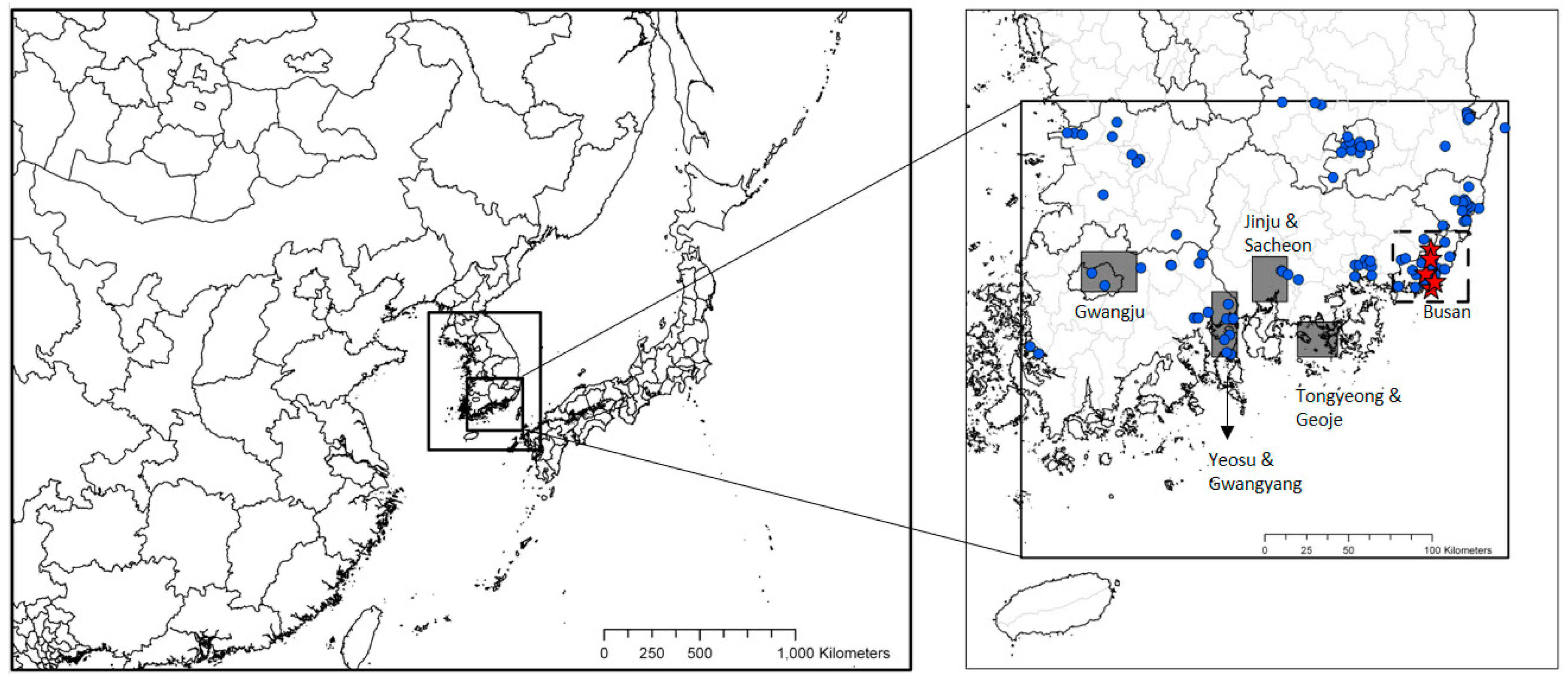
Figure 2.
Box and whisker plot of MDA1O3 values at all monitors in the 3-km modeling domain during August 2007. Blue dots are MDA1O3 values outside the 10–90 percentile range for each day in August 2007. The red line indicates the one-hour Ozone Air Quality Standards (O3AQS) level.
Figure 2.
Box and whisker plot of MDA1O3 values at all monitors in the 3-km modeling domain during August 2007. Blue dots are MDA1O3 values outside the 10–90 percentile range for each day in August 2007. The red line indicates the one-hour Ozone Air Quality Standards (O3AQS) level.

Figure 3.
Modeled and observed 2-m temperatures (a), 10-m wind speeds (b), and cloud fractions (c) averaged spatially for the 3-km domain.
Figure 3.
Modeled and observed 2-m temperatures (a), 10-m wind speeds (b), and cloud fractions (c) averaged spatially for the 3-km domain.

Figure 4.
Spatial distribution of period average NOx emissions (a) and hourly domain-wide total NOx emissions (b) for 3-km domain.
Figure 4.
Spatial distribution of period average NOx emissions (a) and hourly domain-wide total NOx emissions (b) for 3-km domain.

Figure 5.
Period average isoprene emissions modeled by (a) MEGAN and (b) BEIS3 in tons per day (TPD). MEGAN: Model of Emissions of Gases and Aerosols from Nature; BEIS3: Biogenic Emissions Inventory System Version 3.
Figure 5.
Period average isoprene emissions modeled by (a) MEGAN and (b) BEIS3 in tons per day (TPD). MEGAN: Model of Emissions of Gases and Aerosols from Nature; BEIS3: Biogenic Emissions Inventory System Version 3.

Figure 6.
Hourly modeled (red lines for MEGAN and blue lines for BEIS3) and observed (black dots) isoprene concentrations at five PAMS sites.
Figure 6.
Hourly modeled (red lines for MEGAN and blue lines for BEIS3) and observed (black dots) isoprene concentrations at five PAMS sites.
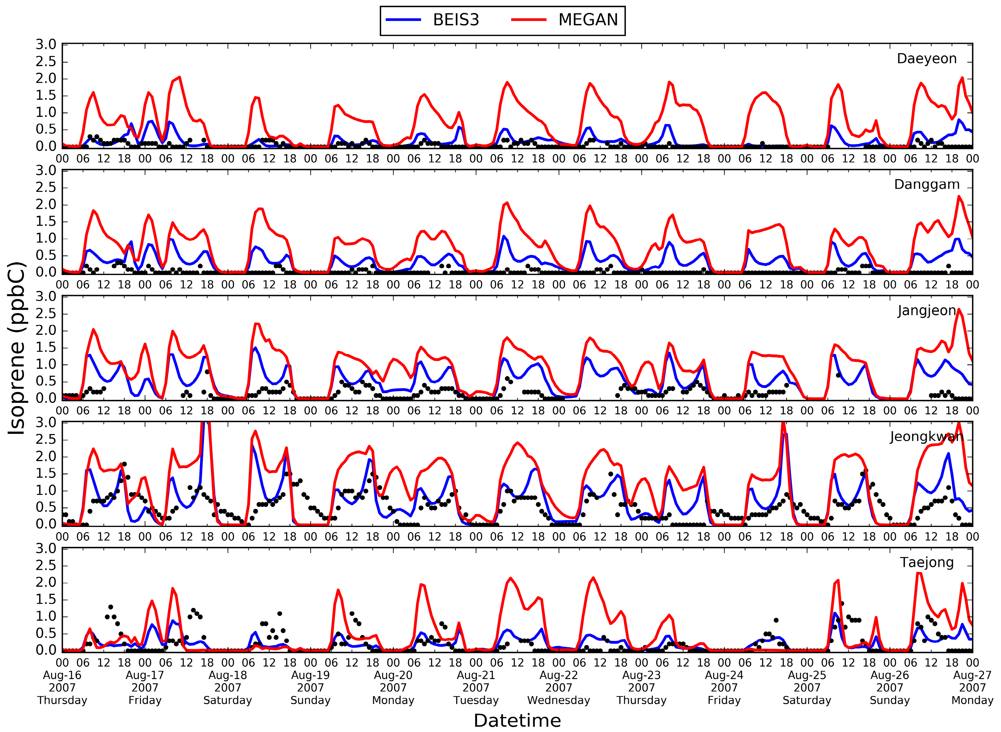
Figure 7.
Modeled and observed NOx and O3 concentrations at (A) a monitor near Busan and (B) another monitor in Gwangju where the model shows good or poor performance, respectively.
Figure 7.
Modeled and observed NOx and O3 concentrations at (A) a monitor near Busan and (B) another monitor in Gwangju where the model shows good or poor performance, respectively.

Figure 8.
MDA1O3 estimated with CMAQ-MEGAN (left) and differences between CMAQ-MEGAN and CMAQ-BEIS3 (right): (A) 17 August; (B) 18 August; (C) 24 August; and (D) 25 August 2007.
Figure 8.
MDA1O3 estimated with CMAQ-MEGAN (left) and differences between CMAQ-MEGAN and CMAQ-BEIS3 (right): (A) 17 August; (B) 18 August; (C) 24 August; and (D) 25 August 2007.


Figure 9.
One-hour ozone concentrations estimated with CMAQ-MEGAN (left) and differences between CMAQ-MEGAN and CMAQ-BEIS3 (right) in 2007: (A) 5 PM on 17 August; (B) 3 PM on 18 August; (C) 4 PM on 24 August; and (D) 3 PM on 25 August.
Figure 9.
One-hour ozone concentrations estimated with CMAQ-MEGAN (left) and differences between CMAQ-MEGAN and CMAQ-BEIS3 (right) in 2007: (A) 5 PM on 17 August; (B) 3 PM on 18 August; (C) 4 PM on 24 August; and (D) 3 PM on 25 August.
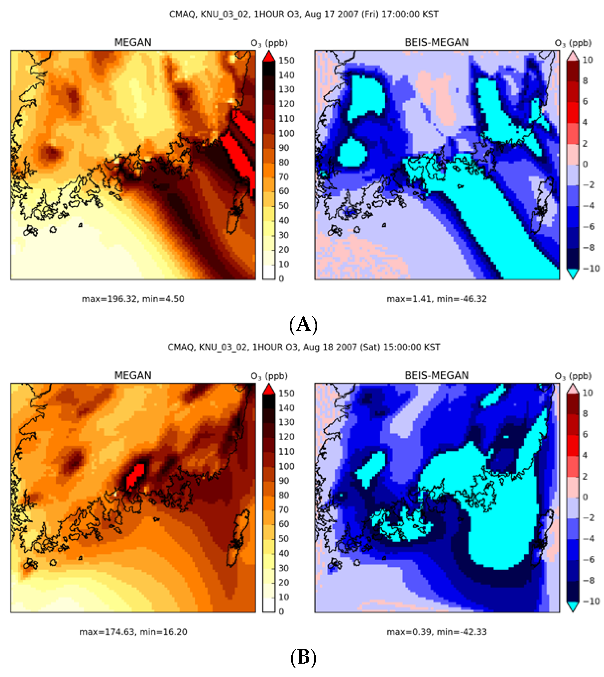
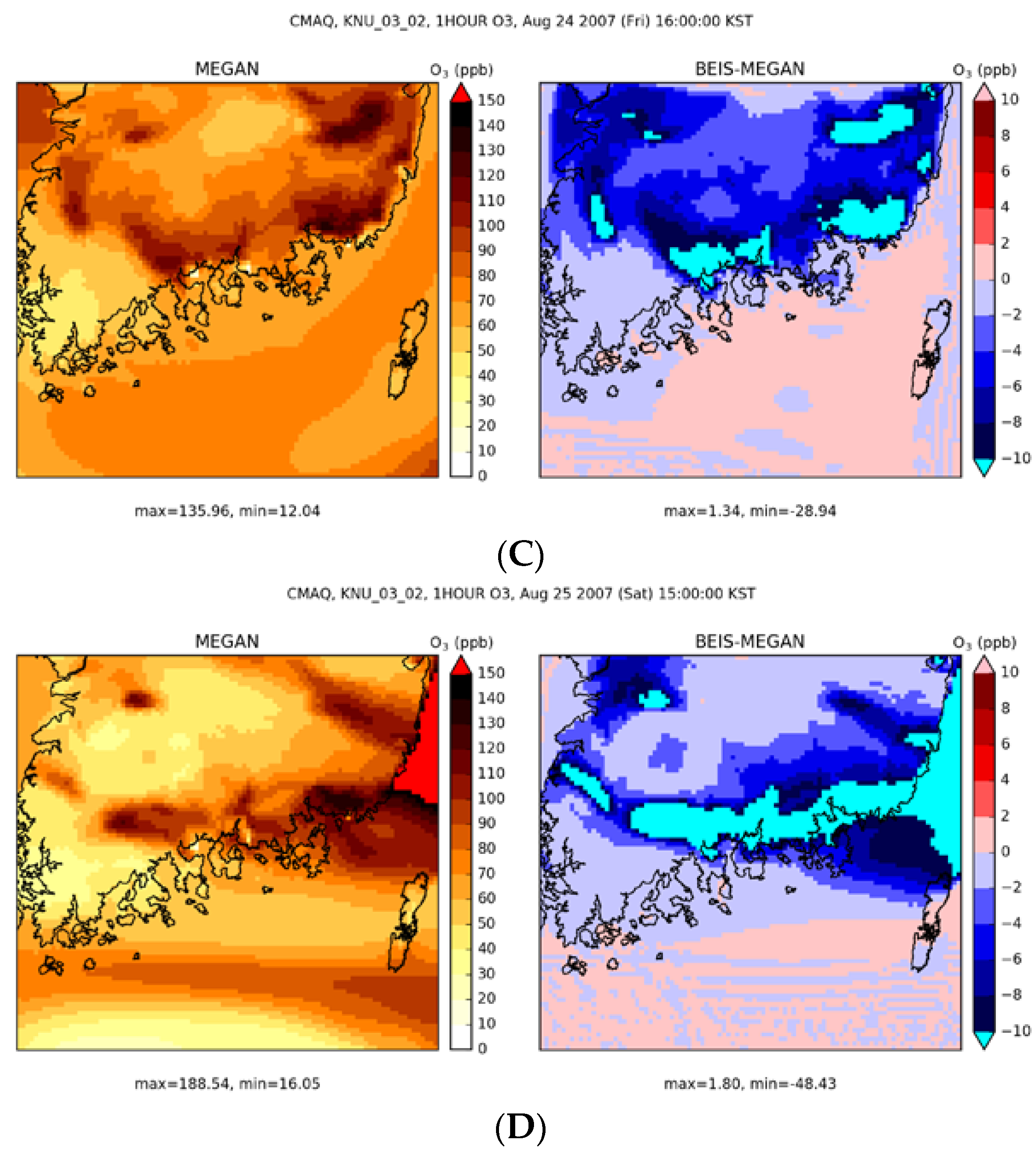
Figure 10.
MDA8O3 estimated with CMAQ-MEGAN (left) and differences between CMAQ-MEGAN and CMAQ-BEIS3 (right): (A) 17 August; (B) 18 August; (C) 24 August; and (D) 25 August 2007.
Figure 10.
MDA8O3 estimated with CMAQ-MEGAN (left) and differences between CMAQ-MEGAN and CMAQ-BEIS3 (right): (A) 17 August; (B) 18 August; (C) 24 August; and (D) 25 August 2007.
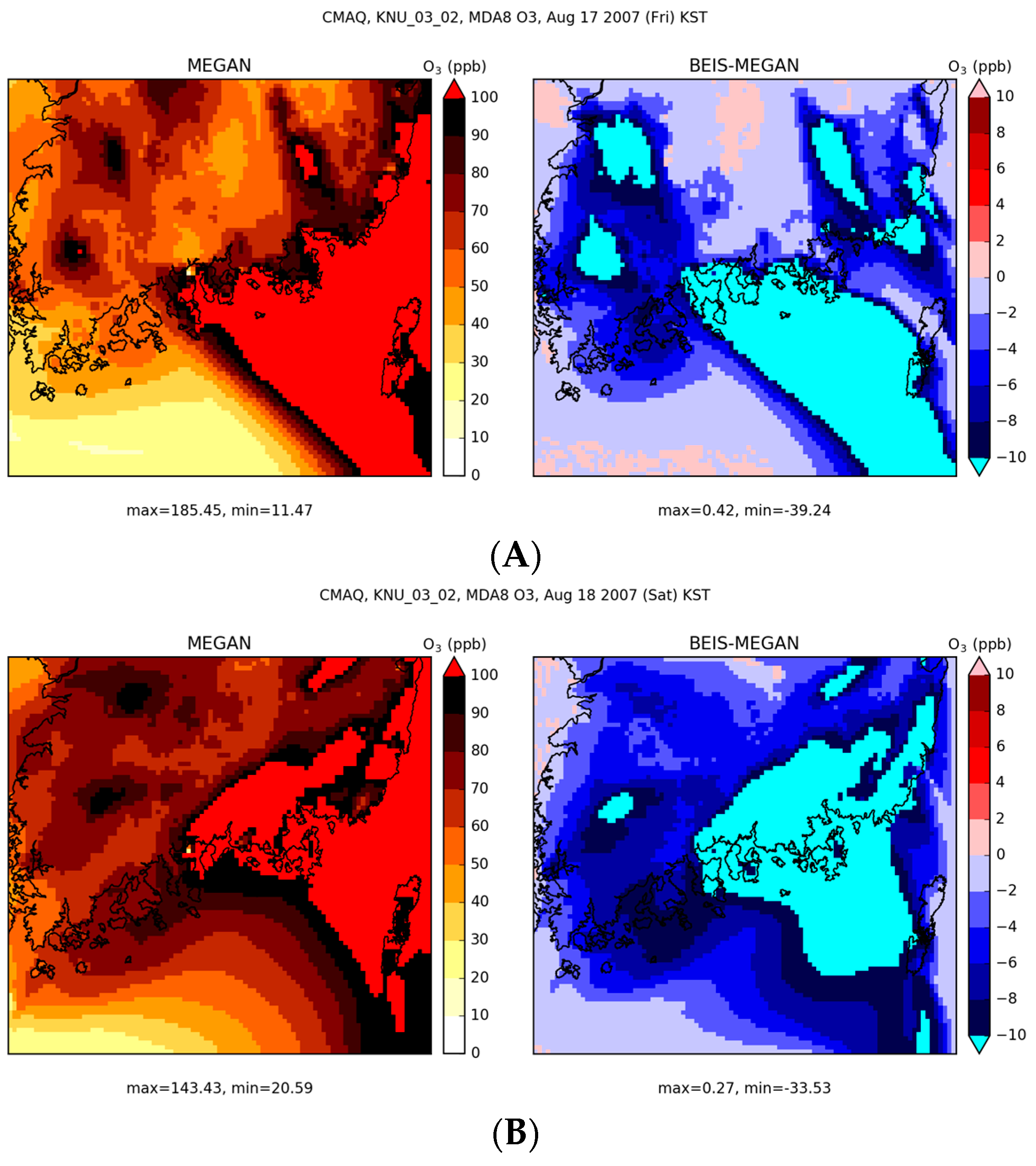

Figure 11.
The first-order sensitivity coefficients to changes in NOx at (A) 5 PM on 17 August, (B) 3 PM on 18 August 2007 (C) 4 PM on 24 August, and (D) 3 PM on 25 August.
Figure 11.
The first-order sensitivity coefficients to changes in NOx at (A) 5 PM on 17 August, (B) 3 PM on 18 August 2007 (C) 4 PM on 24 August, and (D) 3 PM on 25 August.

Figure 12.
Ozone sensitivity to a 30% reduction in anthropogenic NOx with biogenic emissions estimated by MEGAN (left) and BEIS3 (right): (A) 5PM on 17 August; (B) 3 PM on 18 August; (C) 4 PM on 24 August; and (D) 3 PM on 25 August 2007.
Figure 12.
Ozone sensitivity to a 30% reduction in anthropogenic NOx with biogenic emissions estimated by MEGAN (left) and BEIS3 (right): (A) 5PM on 17 August; (B) 3 PM on 18 August; (C) 4 PM on 24 August; and (D) 3 PM on 25 August 2007.

Figure 13.
Ozone isopleth for major cities in the modeling domain at selected hours: (A) Gwangju with MEGAN, (B) Gwangju with BEIS3, (C) Tongyeong and Geoje with MEGAN, (D) Tongyeong and Geoje with BEIS3, (E) Jinju and Sacheon with MEGAN, (F) Jinju and Sacheon with BEIS3, (G) Yeosu and Gwangyang with MEGAN, and (H) Yeosu and Gwangyang with BEIS3. Dotted blue lines represent the ridgeline when at given NOx emission, ENOx. The arrows in (F) illustrate ozone concentration changes with NOx emission reductions from 0% to 10% or 20%.


Figure 14.
Relative changes in eight-hour maximum ozone because of anthropogenic emissions reduction with MEGAN (black) and BEIS (gray) estimated biogenic emissions: (a) 30% NOx reduction, (b) 30% VOCs reduction, and (c) both 30% NOx and 30% VOCs reduction.
Figure 14.
Relative changes in eight-hour maximum ozone because of anthropogenic emissions reduction with MEGAN (black) and BEIS (gray) estimated biogenic emissions: (a) 30% NOx reduction, (b) 30% VOCs reduction, and (c) both 30% NOx and 30% VOCs reduction.

Table 1.
Number of monitor-days in the southern part of South Korea during 2007 when maximum daily one-hour ozone concentration (MDA1O3) was over 100 ppb.
Table 1.
Number of monitor-days in the southern part of South Korea during 2007 when maximum daily one-hour ozone concentration (MDA1O3) was over 100 ppb.
| Month of 2007 | Number of Monitor-Days When MDA1O3 > 100 ppb |
|---|---|
| March | 3 |
| April | 16 |
| May | 49 |
| June | 24 |
| July | 32 |
| August | 58 |
| September | 24 |
| October | 1 |
© 2017 by the authors. Licensee MDPI, Basel, Switzerland. This article is an open access article distributed under the terms and conditions of the Creative Commons Attribution (CC BY) license (http://creativecommons.org/licenses/by/4.0/).
Share and Cite
MDPI and ACS Style
Kim, E.; Kim, B.-U.; Kim, H.C.; Kim, S. The Variability of Ozone Sensitivity to Anthropogenic Emissions with Biogenic Emissions Modeled by MEGAN and BEIS3. Atmosphere 2017, 8, 187. https://doi.org/10.3390/atmos8100187
AMA Style
Kim E, Kim B-U, Kim HC, Kim S. The Variability of Ozone Sensitivity to Anthropogenic Emissions with Biogenic Emissions Modeled by MEGAN and BEIS3. Atmosphere. 2017; 8(10):187. https://doi.org/10.3390/atmos8100187
Chicago/Turabian StyleKim, Eunhye, Byeong-Uk Kim, Hyun Cheol Kim, and Soontae Kim. 2017. "The Variability of Ozone Sensitivity to Anthropogenic Emissions with Biogenic Emissions Modeled by MEGAN and BEIS3" Atmosphere 8, no. 10: 187. https://doi.org/10.3390/atmos8100187
Note that from the first issue of 2016, this journal uses article numbers instead of page numbers. See further details here.