
Mountain Waves in High Resolution Forecast Models: Automated Diagnostics of Wave Severity and Impact on Surface Winds

Abstract
:1. Introduction
2. Materials and Methods
2.1. The Met Office Unified Model and UKV Configuration
2.2. The 3DVOM Model
2.3. BAe-146 Aircraft Observations
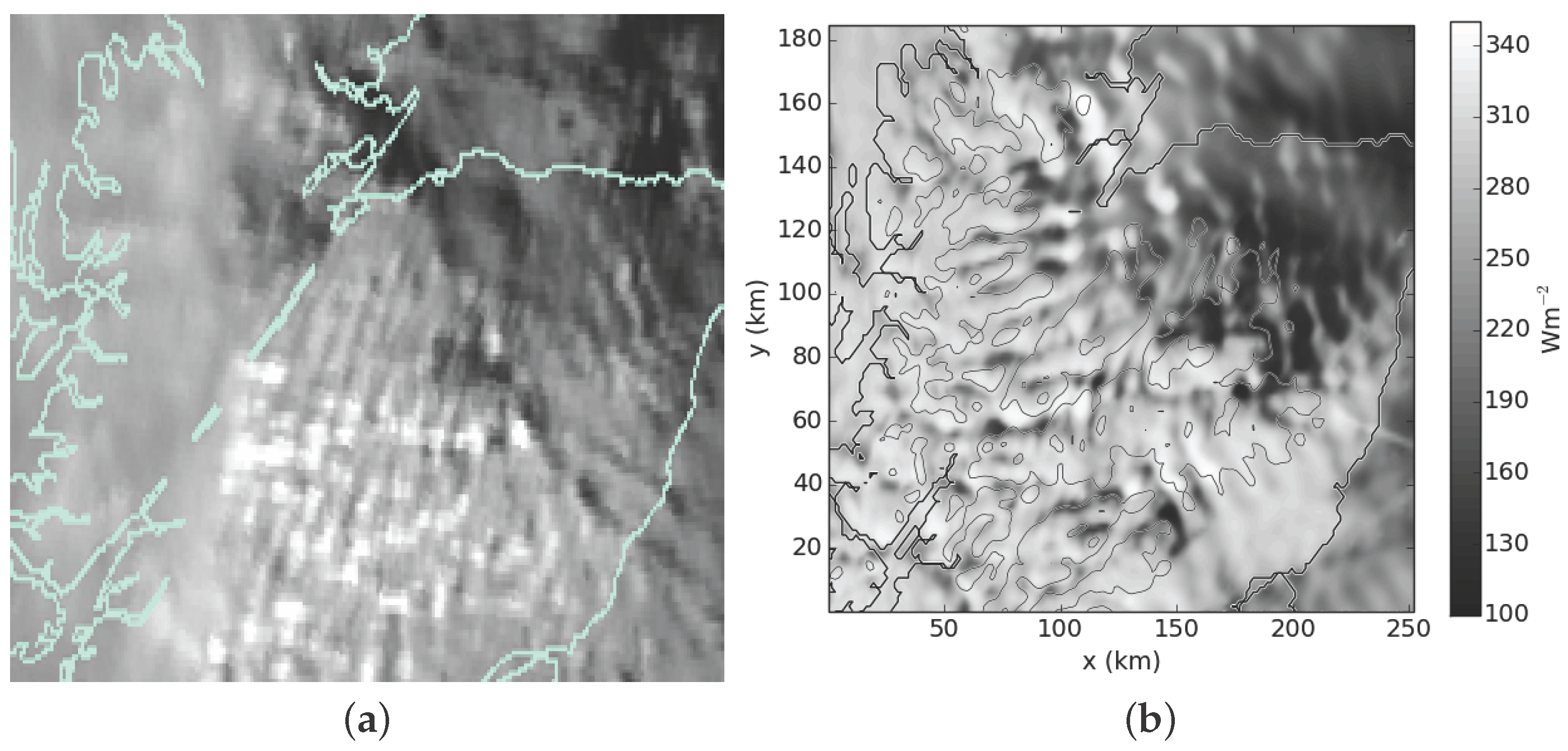
2.3.1. Instrumentation
2.3.2. Calibration and Quality Control
2.3.3. Flight Day
3. Results
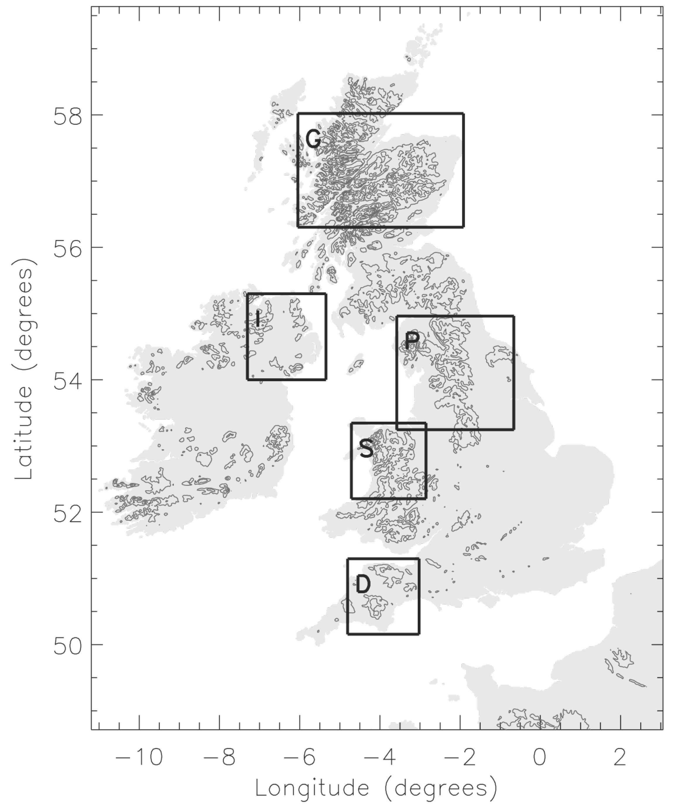
3.1. Lee Wave Statistics
3.2. Diagnosis of Rotor-Like Patterns in Modelled Near-Surface Winds
- (i)
- || > 5 ms and lee waves of moderate or greater amplitude diagnosed
- (ii)
- andor
- (iii)
- + 0.1 ms
3.3. Simulation of Lee Waves within UKV
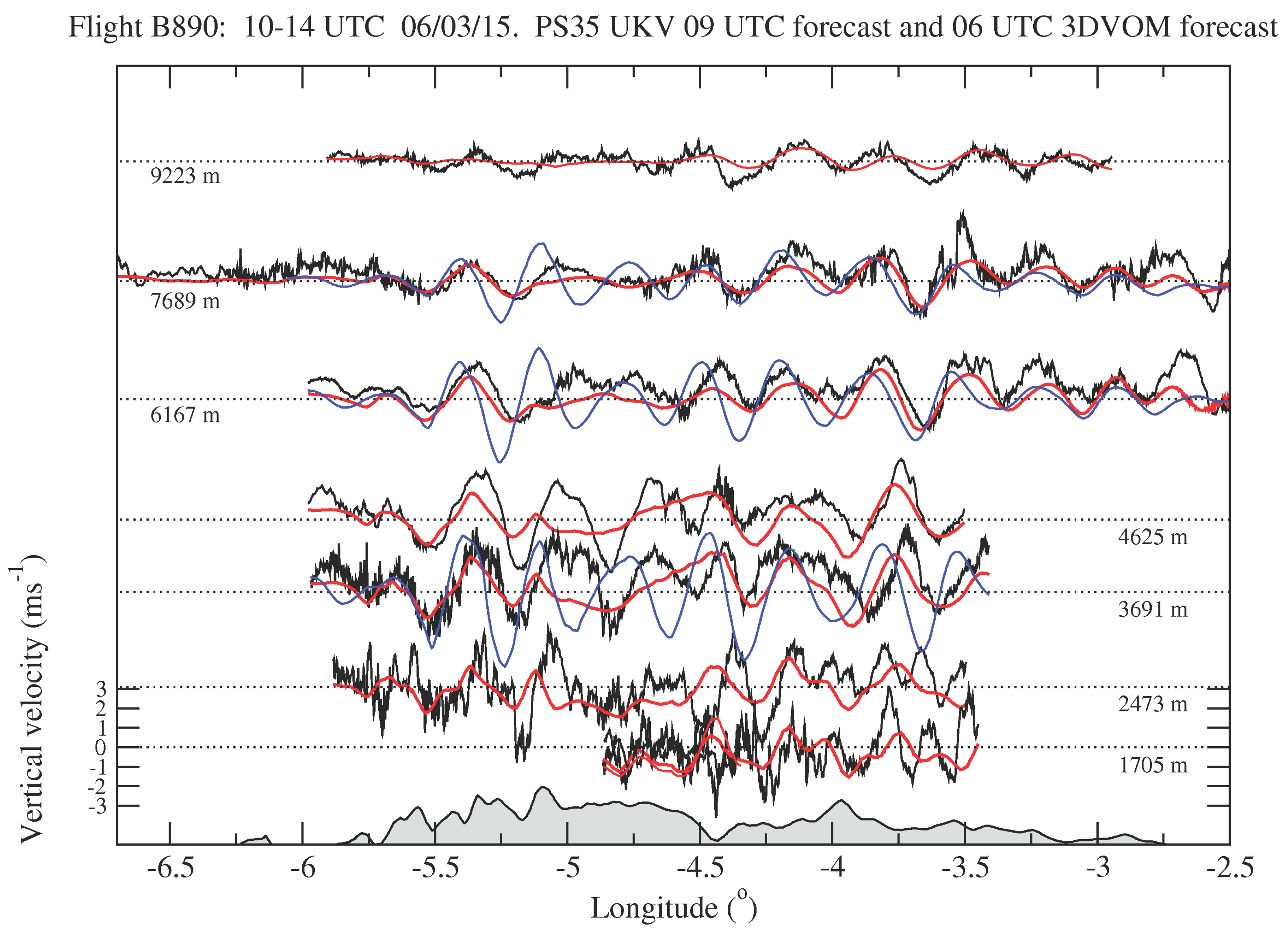
3.3.1. Case Study: 6 March 2015
4. Discussion
- No simplifying (linear) approximations applied to the model equations of motion; the most hazardous mountain wave flows are highly non-linear, e.g., rotors and hydraulic jumps/wave breaking
- Realistic initial and boundary conditions, data assimilation, representation of convergence and convection; problems can occur in 3DVOM when there is significant horizontal variation in conditions and atmospheric forcing (e.g., trough or low centre within the domain), since it is initialised by a single profile
- Thorough representation of moist processes (noting that the U.K. has a very moist climate with cloud and rainfall common); 3DVOM is a dry model, but in reality, reversible latent heating (cloud formation and evaporation) effects favour flow over terrain rather than blocking, also affecting wave amplitude [58]; meanwhile, irreversible latent heating effects (e.g., upslope rainfall) modify the stability profile and, hence, the wave response [59,60,61,62]; further, any orographically-triggered deep convection will negate wave activity
- Direct simulation of the diurnal cycle through radiation, surface and boundary layer parametrisations, including for instance nocturnal stable boundary layers; boundary layer stability strongly affects wave propagation and lee wave decay [64]
- Full and contiguous coverage of the U.K. (and eventually beyond, as future computing resources allow)
- Lee wave impacts become prognostic; the interplay of lee waves with the atmospheric environment in which they form, including other weather phenomena, is represented
- Access to a comprehensive, standardised set of diagnostics, long-term central archiving
5. Conclusions
Acknowledgments
Author Contributions
Conflicts of Interest
References
- Holmboe, J.R.; Klieforth, H. Investigation of Mountain Lee Waves and the Airflow over the Sierra Nevada; Final Report; UCLA: Department of Meteorology, University of California, CA, USA, 1957. [Google Scholar]
- Lilly, D.K.; Zipser, E.J. The front range windstorm of 11 January 1972—A meteorological narrative. Weatherwise 1972, 25, 56–63. [Google Scholar] [CrossRef]
- Durran, D.R. Another look at downslope windstorms. Part I: The development of analogs to supercritical flow in an infinitely deep, continuously stratified fluid. J. Atmos. Sci. 1986, 43, 2527–2543. [Google Scholar] [CrossRef]
- Jiang, Q.; Doyle, J.D. Diurnal Variation of Downslope Winds in Owens Valley during the Sierra Rotor Experiment. Mon. Weather Rev. 2008, 136, 3760–3780. [Google Scholar] [CrossRef]
- Peltier, W.R.; Clark, T.L. The evolution and stability of finite-amplitude mountain waves. Part II: Surface wave drag and severe downslope windstorms. J. Atmos. Sci. 1979, 36, 1498–1529. [Google Scholar] [CrossRef]
- Lin, Y.L.; Wang, T.A. Flow regimes and transient dynamics of two-dimensional stratifed flow over an isolated mountain ridge. J. Atmos. Sci. 1996, 53, 139–158. [Google Scholar] [CrossRef]
- Clark, T.L.; Hall, W.D.; Kerr, R.M.; Middleton, D.; Radke, L.; Martin, F.; Neiman, P.J.; Levinson, D. Origins of aircraft-damaging clear-air turbulence during the 9 December 1992 Colorado downslope windstorm: Numerical simulations and comparison with observations. J. Atmos. Sci. 2000, 57, 1105–1131. [Google Scholar] [CrossRef]
- Jiang, Q.; Doyle, J.D. Gravity Wave Breaking over the Central Alps: Role of Complex Terrain. J. Atmos. Sci. 2004, 61, 2249–2266. [Google Scholar] [CrossRef]
- Doyle, J.D.; Shapiro, M.A.; Jiang, Q.; Bartels, D.L. Large-Amplitude Mountain Wave Breaking over Greenland. J. Atmos. Sci. 2005, 62, 3106–3126. [Google Scholar] [CrossRef]
- Belusic, D.; Zagar, M.; Grisogono, B. Numerical simulation of pulsations in the bora wind. Q. J. R. Meteorol. Soc. 2007, 133, 1371–1388. [Google Scholar] [CrossRef]
- Doyle, J.D.; Durran, D.R. The dynamics of mountain-wave-induced rotors. J. Atmos. Sci. 2002, 59, 186–201. [Google Scholar] [CrossRef]
- Vosper, S.B. Inversion effects on mountain lee waves. Q. J. R. Meteorol. Soc. 2004, 130, 1723–1748. [Google Scholar] [CrossRef]
- Vosper, S.B.; Sheridan, P.F.; Brown, A.R. Flow separation and rotor formation beneath two-dimensional trapped lee waves. Q. J. R. Meteorol. Soc. 2006, 132, 2415–2438. [Google Scholar] [CrossRef]
- Sheridan, P.F.; Horlacher, V.; Rooney, G.G.; Hignett, P.; Mobbs, S.D.; Vosper, S.B. Influence of lee waves on the near-surface flow downwind of the Pennines. Q. J. R. Meteorol. Soc. 2007, 133, 1353–1369. [Google Scholar] [CrossRef]
- Sachsperger, J.; Serafin, S.; Grubisic, V. Dynamics of rotor formation in uniformly stratified two-dimensional flow over a mountain. Q. J. R. Meteorol. Soc. 2016, 142, 1201–1212. [Google Scholar] [CrossRef]
- Strauss, L.; Serafin, S.; Haimov, S.; Grubisic, V. Turbulence in breaking mountain waves and atmospheric rotors estimated from airborne in situ and Doppler radar measurements. Q. J. R. Meteorol. Soc. 2015, 141, 3207–3225. [Google Scholar] [CrossRef] [PubMed]
- Strauss, L.; Serafin, S.; Grubisic, V. Atmospheric Rotors and Severe Turbulence in a Long Deep Valley. J. Atmos. Sci. 2016, 73, 1481–1506. [Google Scholar] [CrossRef]
- Hertenstein, R.F.; Kuettner, J. Rotor types associated with steep lee topography: Influence of the wind profile. Tellus A 2005, 57, 117–135. [Google Scholar] [CrossRef]
- Grisogono, B.; Belusic, D. A review of recent advances in understanding the meso- and micro-scale properties of the severe Bora wind. Tellus A 2009, 61, 1–16. [Google Scholar] [CrossRef]
- Agustsson, H.; Olafsson, H. Mean gust factors in complex terrain. Meteorol. Z. 2004, 13, 149–155. [Google Scholar]
- Scorer, R.S. Theory of waves in the lee of mountains. Q. J. R. Meteorol. Soc. 1949, 75, 41–56. [Google Scholar] [CrossRef]
- Shutts, G.J. Operational lee wave forecasting. Meteorol. Appl. 1997, 4, 23–35. [Google Scholar] [CrossRef]
- Doyle, J.D.; Durran, D.R. Recent developments in the theory of atmospheric rotors. Bull. Am. Meteorol. Soc. 2004, 85, 337–342. [Google Scholar] [CrossRef]
- Doyle, J.D.; Durran, D.R. Rotor and subrotor dynamics in the lee of three-dimensional terrain. J. Atmos. Sci. 2007, 64, 4202–4221. [Google Scholar] [CrossRef]
- Doyle, J.D.; Grubisic, V.; Brown, W.O.J.; Wekker, S.F.J.D.; Doernbrack, A.; Jiang, Q.; Mayor, S.D.; Weissmann, M. Observations and numerical simulations of subrotor vortices during T-REX. J. Atmos. Sci. 2009, 66, 1224–1249. [Google Scholar] [CrossRef]
- Knigge, C.; Etling, D.; Pacib, A.; Eiff, O. Laboratory experiments on mountain-induced rotors. Q. J. R. Meteorol. Soc. 2010, 136, 442–450. [Google Scholar] [CrossRef]
- Teixeira, M. Diagnosing Lee Wave Rotor Onset Using a Linear Model Including a Boundary Layer. Atmosphere 2017, 8, 5. [Google Scholar] [CrossRef]
- Mobbs, S.D.; Vosper, S.B.; Sheridan, P.F.; Cardoso, R.; Burton, R.R.; Arnold, S.J.; Hill, M.K.; Horlacher, V.; Gadian, A.M. Observations of downslope winds and rotors in the Falkland Islands. Q. J. R. Meteorol. Soc. 2005, 131, 329–351. [Google Scholar] [CrossRef]
- Sheridan, P.F.; Vosper, S.B. A flow regime diagram for forecasting lee waves, rotors and downslope winds. Meteorol. Appl. 2006, 13, 179–195. [Google Scholar] [CrossRef]
- Sheridan, P.F.; Vosper, S.B. Numerical simulations of rotors, hydraulic jumps and eddy shedding in the Falkland Islands. Atmos. Sci. Lett. 2006, 6, 211–218. [Google Scholar] [CrossRef]
- Mayr, G.J.; Armi, L. The Influence of Downstream Diurnal Heating on the Descent of Flow across the Sierras. J. Appl. Meteorol. Climatol. 2010, 49, 1906–1912. [Google Scholar] [CrossRef]
- Webster, S.; Brown, A.R.; Cameron, D.R.; Jones, C.P. Improvements to the representation of orography in the Met Office Unified Model. Q. J. R. Meteorol. Soc. 2003, 129, 1989–2010. [Google Scholar] [CrossRef]
- Turner, J. Development of a Mountain Wave Turbulence Prediction Scheme for Civil Aviation; Forecasting Research Technical Report No. 265; Met Office: Exeter, UK, 1999. [Google Scholar]
- Sharman, R.; Tebaldi, C.; Wiener, G.; Wolff, J. An integrated approach to mid- and upper-level turbulence forecasting. Weather Forecast. 2006, 21, 268–287. [Google Scholar] [CrossRef]
- Gill, P.G. Objective verification of World Area Forecast Centre clear air turbulence forecasts. Meteorol. Appl. 2014, 21, 3–11. [Google Scholar] [CrossRef]
- Teixeira, M.; Argain, J.L.; Miranda, P.M.A. Orographic Drag Associated with Lee Waves Trapped at an Inversion. J. Atmos. Sci. 2013, 20, 2930–2947. [Google Scholar] [CrossRef]
- Wong, W.K.; Lau, C.S.; Chan, P.W. Aviation model: A fine-scale numerical weather prediction system for aviation applications at the Hong Kong International Airport. Adv. Meteorol. 2013, 2013, 532475. [Google Scholar] [CrossRef]
- Chan, P.W.; Hon, K.K. Performance of super high resolution numerical weather prediction model in forecasting terrain-disrupted airflow at the Hong Kong International Airport: Case studies. Meteorol. Appl. 2016, 23, 101–114. [Google Scholar] [CrossRef]
- Li, L.; Chan, P.W. Numerical simulation study of the effect of buildings and complex terrain on the low-level winds at an airport in typhoon situation. Meteorol. Z. 2012, 21, 183–192. [Google Scholar]
- Carruthers, D.; Ellis, A.; Chan, J.H.P.W. Modelling of wind shear downwind of mountain ridges at Hong Kong International Airport. Meteorol. Appl. 2014, 21, 94–104. [Google Scholar] [CrossRef]
- Rasheed, A.; Suld, J.K.; Kvamsdala, T. A Multiscale Wind and Power Forecast System for Wind Farms. Energy Procedia 2014, 53, 290–299. [Google Scholar] [CrossRef]
- Vosper, S.B. Development and testing of a high resolution mountain-wave forecasting system. Meteorol. Appl. 2003, 10, 75–86. [Google Scholar] [CrossRef]
- Vosper, S.B.; Worthington, R.M. VHF radar measurements and model simulations of mountain waves over Wales. Q. J. R. Meteorol. Soc. 2002, 128, 185–204. [Google Scholar] [CrossRef]
- Vosper, S.B.; Wells, H.; Sinclair, J.A.; Sheridan, P.F. A climatology of lee waves over the UK derived from model forecasts. Meteorol. Appl. 2013, 20, 466–481. [Google Scholar] [CrossRef]
- Grubisic, V.; Doyle, J.D.; Kuettner, J.; Mobbs, S.; Smith, R.B.; Whiteman, C.D.; Dirks, R.; Czyzyk, S.; Cohn, S.A.; Vosper, S.; et al. The Terrain-Induced Rotor Experiment: A field campaign overview including observational highlights. Bull. Am. Meteor. Soc. 2008, 89, 1513–1533. [Google Scholar] [CrossRef]
- Casswell, S.A. A simplified calculation of maximum vertical velocities in mountain lee waves. Meteorol. Mag. 1966, 95, 68–80. [Google Scholar]
- Agustsson, H.; Olafsson, H. Simulating a severe windstorm in complex terrain. Meteorol. Z. 2007, 16, 111–122. [Google Scholar]
- Agustsson, H.; Olafsson, H. The bimodal downslope windstorms at Kvisker. Meteorol. Atmos. Phys. 2012, 116, 27–42. [Google Scholar] [CrossRef]
- Agustsson, H.; Olafsson, H. Simulations of observed lee waves and rotor turbulence. Mon. Weather Rev. 2014, 142, 832–849. [Google Scholar] [CrossRef]
- Tang, Y.; Lean, H.W.; Bornemann, J. The benefits of the Met Office variable resolution NWP model for forecasting convection. Meteorol. Appl. 2013, 20, 417–426. [Google Scholar] [CrossRef]
- Wood, N.; Staniforth, A.; White, A.; Allen, T.; Diamantakis, M.; Gross, M.; Melvin, T.; Smith, C.; Vosper, S.; Zerroukat, M.; et al. An inherently mass-conserving semi-implicit semi-Lagrangian discretisation of the deep-atmosphere global nonhydrostatic equations. Q. J. R. Meteorol. Soc. 2014, 140, 1505–1520. [Google Scholar] [CrossRef]
- Sheridan, P.F.; Vosper, S.B. High-resolution simulations of lee waves and downslope winds over the Sierra Nevada during T-REX IOP 6. J. Appl. Meteorol. Climatol. 2012, 51, 1333–1352. [Google Scholar] [CrossRef]
- Doyle, J.D.; Gabersek, S.; Jiang, Q.; Bernardet, L.; Brown, J.M.; Dornbrack, A.; Filause, E.; Grubisic, V.; Kirshbaum, D.J.; Knoth, O.; et al. Mountain-Wave Simulations and Implications for Mesoscale Predictability. Mon. Weather Rev. 2011, 139, 2811–2831. [Google Scholar] [CrossRef]
- Renfrew, I.A.; Outten, S.D.; Moore, G.W.K. An easterly tip jet off Cape Farewell, Greenland. I: Aircraft observations. Q. J. R. Meteorol. Soc. 2009, 135, 1919–1933. [Google Scholar] [CrossRef] [Green Version]
- Petersen, G.N.; Renfrew, I.A. Aircraft-based observations of air-sea fluxes over Denmark Strait and the Irminger Sea during high wind speed conditions. Q. J. R. Meteorol. Soc. 2009, 135, 2030–2045. [Google Scholar] [CrossRef]
- Beswick, K.M.; Gallagher, M.W.; Webb, A.R.; Norton, E.G.; Perry, F. Application of the Aventech AIMMS20AQ airborne probe for turbulence measurements during the Convective Storm Initiation Project. Atmos. Chem. Phys. 2008, 8, 5449–5463. [Google Scholar] [CrossRef]
- Khelif, D.; Burns, S.P.; Friehe, C.A. Improved wind measurements on research aircraft. J. Atmos. Ocean. Technol. 1999, 16, 860–875. [Google Scholar] [CrossRef]
- Jiang, Q. Moist dynamics and orographic precipitation. Tellus A 2003, 55, 301–316. [Google Scholar] [CrossRef]
- Doyle, J.D.; Smith, R.B. Mountain waves over the Hohe Tauern: Influence of upstream diabatic effects. Q. J. R. Meteorol. Soc. 2003, 129, 799–823. [Google Scholar] [CrossRef]
- Jiang, Q.; Doyle, J.D. The Impact of Moisture on Mountain Waves during T-REX. Mon. Weather Rev. 2009, 137, 3888–3906. [Google Scholar] [CrossRef]
- Worthington, R.M. Radar measurement of the effect of boundary-layer saturation on mountain-wave amplitude. Meteorol. Atmos. Phys. 2009, 105, 29–35. [Google Scholar] [CrossRef]
- Rognvaldsson, O.; Bao, J.W.; Agustsson, H.; Olafsson, H. Downslope windstorm in Iceland—WRF/MM5 model comparison. Atmos. Chem. Phys. 2011, 11, 103–120. [Google Scholar] [CrossRef]
- Smith, R.B.; Jiang, Q.; Doyle, J.D. A theory of gravity wave absorption by boundary layers. J. Atmos. Sci. 2006, 63, 774–781. [Google Scholar] [CrossRef]
- Jiang, Q.; Smith, R.B.; Doyle, J.D. Interaction between trapped waves and boundary layers. J. Atmos. Sci. 2006, 63, 617–633. [Google Scholar] [CrossRef]
- Smith, R.B. Interacting Mountain Waves and Boundary Layers. J. Atmos. Sci. 2007, 64, 594–607. [Google Scholar] [CrossRef]
- Sheridan, P. Review of Techniques and Research for Gust Forecasting and Parameterisation; Forecasting Research Technical Report No. 570; Met Office: Exeter, UK, 2011. [Google Scholar]
- Mirza, A.K.; Ballard, S.P.; Dance, S.L.; Maisey, P.; Rooney, G.G.; Stone, E.K. Comparison of aircraft derived observations with in situ research aircraft measurements. Q. J. R. Meteorol. Soc. 2016, 142, 2949–2967. [Google Scholar] [CrossRef]
- Furevik, B.R.; Schyberg, H.; Noer, G.; Tveter, F.; Roehrs, J. ASAR and ASCAT in Polar Low Situations. J. Atmos. Ocean. Technol. 2015, 32, 783–792. [Google Scholar] [CrossRef]


| Case (Figure) | Validity Time (UTC, dd/mm/yy) | Domain | || (ms−1) | (ms−1) | () | Wave sev. | Rotor Risk (Trigger) |
|---|---|---|---|---|---|---|---|
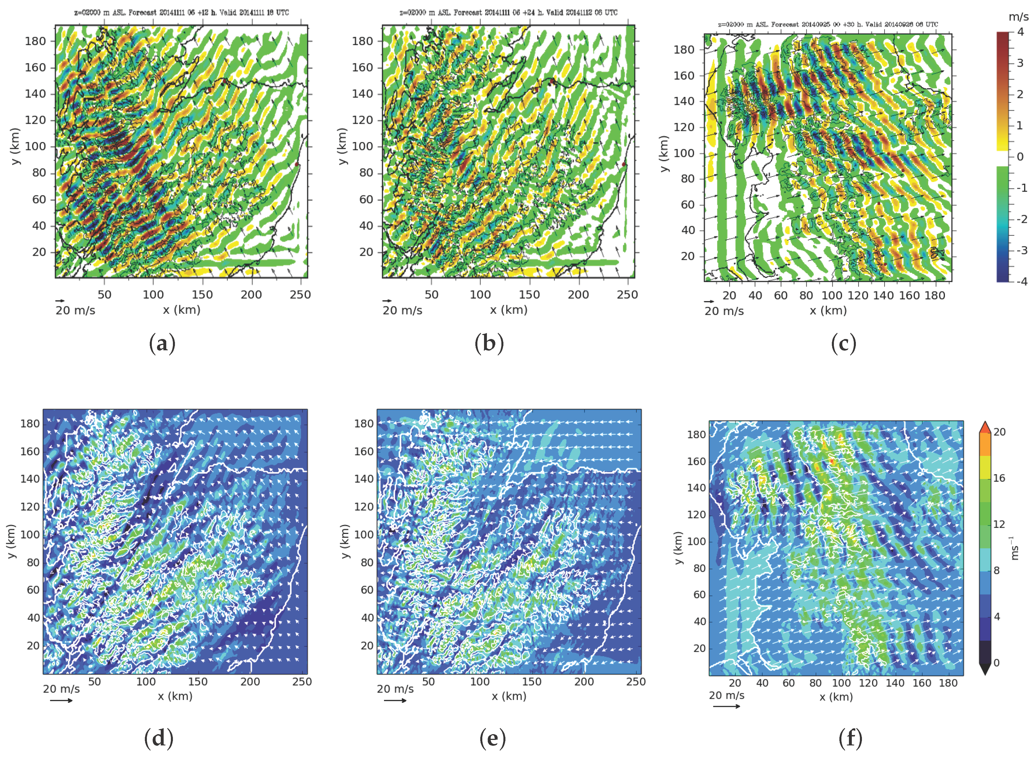
| 1 (4) | 18, 11/11/14 | Grampians | 6.13 | 0.553 | 0.327 (0.250) | severe | yes (w + ) |
| 2 (4) | 06, 12/11/14 | Grampians | 6.35 | 0.288 | 0.249 (0.250) | moderate | no |
| 3 (4) | 06, 25/09/14 | Pennines | 8.03 | 0.429 | 0.211 (0.190) | moderate | yes (w + ) |
| 4 (5) | 00, 18/07/14 | Snowdon | 8.67 | 0.245 | 0.227 (0.180) | moderate | yes () |
| 5 (5) | 06, 03/10/14 | Snowdon | 11.20 | 0.246 | 0.145 (0.180) | moderate | no |
| 6 (5) | 18, 08/05/14 | Dartmoor | 8.44 | 0.301 | 0.145 (0.150) | moderate | yes (w) |
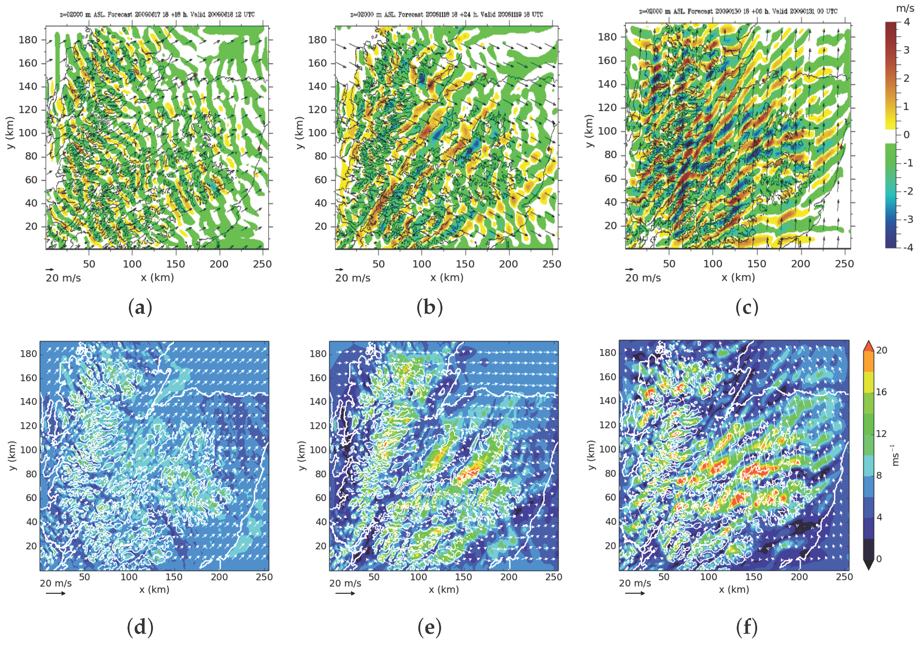
| (2) | 12, 18/06/09 | Grampians | 7.05 | 0.056 | 0.163 (0.250) | nil | no |
| (2) | 18, 19/11/08 | Grampians | 7.02 | 0.262 | 0.383 (0.250) | moderate | yes () |
| (2) | 00, 31/01/09 | Grampians | 7.00 | 0.624 | 0.611 (0.250) | severe | yes (w + ) |
© 2017 by the authors; licensee MDPI, Basel, Switzerland. This article is an open access article distributed under the terms and conditions of the Creative Commons Attribution (CC BY) license (http://creativecommons.org/licenses/by/4.0/).
Share and Cite
Sheridan, P.; Vosper, S.; Brown, P. Mountain Waves in High Resolution Forecast Models: Automated Diagnostics of Wave Severity and Impact on Surface Winds. Atmosphere 2017, 8, 24. https://doi.org/10.3390/atmos8010024
Sheridan P, Vosper S, Brown P. Mountain Waves in High Resolution Forecast Models: Automated Diagnostics of Wave Severity and Impact on Surface Winds. Atmosphere. 2017; 8(1):24. https://doi.org/10.3390/atmos8010024
Chicago/Turabian StyleSheridan, Peter, Simon Vosper, and Philip Brown. 2017. "Mountain Waves in High Resolution Forecast Models: Automated Diagnostics of Wave Severity and Impact on Surface Winds" Atmosphere 8, no. 1: 24. https://doi.org/10.3390/atmos8010024