Predicting PM_2.5 Concentrations at a Regional Background Station Using Second Order Self-Organizing Fuzzy Neural Network

Abstract

This study aims to develop a second order self-organizing fuzzy neural network (SOFNN) to predict the hourly concentrations of fine particulate matter (PM_2.5) for the next 24 h at a regional background station called Shangdianzi (SDZ) in China from 14 to 23 January 2010. The structure of the SOFNN was automatically adjusted according to the sensitivity analysis (SA) of model output and the parameter-learning phase was performed applying a second order gradient (SOG) algorithm. Principal component analysis (PCA) was employed to select the dominating factors for PM_2.5 concentrations as the input variables for the SOFNN. It was found that the dominating variables (relative humidity (RH), pressure (Pre), aerosol optical depth (AOD), wind speed (WS) and wind direction (WD)) extracted by PCA agreed well with the characteristics of PM_2.5 at SDZ where the PM_2.5 concentrations were heavily affected by meteorological parameters and were closely related to AOD. The forecasting results showed that the proposed SOG-SASOFNN performed better than other models with higher coefficient of determination (R²) during both training phase and test phase (0.89 and 0.84, respectively) in predicting PM_2.5 concentrations at SDZ. In conclusion, the developed SOG-SASOFNN provided satisfying results for modeling the hourly distribution of PM_2.5 at SDZ during the studied period.

1. Introduction

China has suffered from conspicuously rising air pollution due to the rapid urbanization since 1980s. Gaseous and particulate emissions from various anthropogenic sources such as coal combustion, motor vehicles and industrial processes lead to poor air quality (AQ) [1]. One of the most harmful pollutants is known as fine particulate matter (PM_2.5), a complex mixture of particles with aerodynamic diameters of 2.5 μm or less [2]. Chronic exposure to ambient PM_2.5 causes the public to be faced with increased morbidity and mortality as it can lodge deeply into the lungs [3,4]. In Atlanta, a 10 μg/m³ increase of PM_2.5 is associated with 3.3% increases in emergency department visits for cardiovascular disease [5] and 1.6% increases for respiratory disease [6]. In addition, aerosols affect climate change in a way that a dramatic emission reduction (35%–80%) in anthropogenic aerosols results in approximately 1 °C of extra warming and approximately 0.1 mm·day⁻¹ of extra precipitation globally averaged by the end of the 21st century [7]. Moreover, visibility and PM_2.5 are negatively correlated with Pearson correlations of −0.663 for a regional background station in the boundary of North China Plain (NCP) [8]. In order to take preventive and regulatory measures to manage AQ as well as to provide specific information about concentrations of PM_2.5 with the public, it is necessary to develop methods that can predict PM_2.5 concentrations precisely.

Modeling of the real world processes such as forecasting of AQ has proven to be tough due to their highly chaotic and nonlinear phenomenon [9,10]. Generally, models used to estimate air pollutants comprise process-based methods and data-driven statistical methods [11]. The first class of methods is based on chemical transport models (CTMs) which model the atmospheric and chemical processes involved in the production of an air pollutant [12]. Yu et al. [13] evaluated the performance of the Eta-Community Multiscale Air Quality (CMAQ) model in predicting PM_2.5 and its chemical species over the eastern United States, where the model captured a majority (73%) of PM_2.5 observations within a factor of 2. However, CTMs are complex to implement as they require detailed information on meteorology, emissions inventories and advanced understanding of chemical process. On the contrary, the latter class of methods is driven by satellite readings or ground monitoring measurements [14], thus there is no need for strong assumptions of the underlying air pollution processes during the modeling process. Among the statistical AQ forecasting models, we can mention those based on linear regressions (LR) and neural networks (NNs). Regression models show optimal results when relationship between the predictors (such as meteorological and AQ variables) and the predictand (pollutant concentrations of interest) are almost linear [15]. Regression models are also likely to under predict high concentrations and over predict low concentrations. To overcome some of these limitations, the artificial neural network (ANN), which can be used to derive non-linear functions relating to the predictand and the predictors, has been adopted and proven to be a reliable air pollution modeling tool in many studies [16,17,18]. Chaloulakou et al. [19] analyzed the performance of multiple linear regressions (MLR) and NNs on the forecasting of PM₁₀ in Athens. Ordieres et al. [20] implemented three types of NNs as well as a LR model and a persistence model to forecast daily averages of PM_2.5 in El Paso and Ciudad Juaŕez. The results of both studies clearly demonstrated that NNs were more accurate than LR models for forecasting of concentrations of air pollutants.

Unfortunately, the mapping rules in NNs are not visible and are difficult to understand. That is, one can only ascertain relationships among meteorology and pollutants concentrations data but never be sure about underlying causal mechanism included in the emission and dispersion pattern of air pollutants through NNs. In contrast, fuzzy system (FS) technologies often deal with issues such as reasoning on a high-level than NNs and can handle imprecise information through linguistic expressions [21,22]. Nevertheless, it is difficult to tune the fuzzy rules from the training data for a human operator since FS has limited learning capability. However, the combination of neural network (NN) and FS which leads to fuzzy neural network (FNN) can strength the prediction capabilities compared to using a single methodology [23]. Mishra et al. [24] developed an artificial intelligence based neuro-fuzzy (NF) model to forecast PM_2.5 concentrations during haze hours in Delhi along with MLR and ANN, where NF model performed better in prediction capabilities compared to MLR and ANN.

For fuzzy neural networks (FNNs), the main training process consists of parameter-learning phase and structure-learning phase [25]. However, in most FNNs, only the learning phase of the parameters is determined using supervised or unsupervised learning algorithm and the structure identification is still difficult [26,27]. It is hard for designers to choose the appropriate number of fuzzy rules to forecast air pollutants, especially PM_2.5, applying FNNs with empirically fixed structure. Several early research works have already dealt with self-organizing FNNs (SOFNNs), of which the structure can be adjusted automatically during training process [28]. Habbi et al. [29] used artificial bee colony optimization strategy to find the structure and the parameters of TS fuzzy systems simultaneously. Han et al. [30] developed a sensitivity analysis (SA) of model output based growing-and-pruning approach to generate fuzzy neural model with highly accurate and compact structure. However, as far as we know, few SOFNNs have been applied to estimate the distributions of air pollutants or to forecast the concentrations of PM_2.5.

Therefore, in this paper, the SA based SOFNN (SASOFNN) was used for forecasting the hourly PM_2.5 concentrations of the next 24 h at Shangdianzi (SDZ) station, which is a regional background station located in the boundary of the NCP, from 14 to 23 January 2010. The parameters of the SASOFNN were optimized by a second order gradient (SOG) algorithm with improved training speed and higher approximation accuracy [31,32], as the first order gradient (FOG) algorithm having limited search ability and the genetic algorithm (GA) being very time and computation expensive. Besides, in order to eliminate the irrelevant input parameters, the principal component analysis (PCA) was used to select dominating variables most correlated to PM_2.5 from temperature (T), relative humidity (RH), wind speed (WS), wind direction (WD), pressure (Pre), visibility (Vis), aerosol optical depth (AOD), CO, NO₂, O₃ and SO₂ as the input parameters for the SOG-SASOFNN [33]. It could be found that the dominating variables (RH, Pre, AOD, WS and WD) extracted by PCA coincided with the characteristics of PM_2.5 at SDZ where there were no significant pollution sources within 30 km of the site and the PM_2.5 concentrations were severely influenced by the meteorological parameters and were tightly associated with the AOD. In addition, the prediction performance of the SOG-SASOFNN was analyzed and compared to that of the SASOFNN with FOG algorithm (FOG-SASOFNN) and the echo state network (ESN) in the study of Xu et al. [11] as well as to the Eta-CMAQ modeling results for the hourly PM_2.5 concentrations at the rural sites over the eastern United States from 15 July to 19 August 2004 [13]. The statistical parameters indexes calculated for the models above demonstrated that the SOG-SASOFNN performed better than the FOG-SASOFNN, the ESN and the Eta-CMAQ in predicting the hourly concentrations of PM_2.5. It can be concluded that the SOG-SASOFNN presented here is valid for estimating the hourly distribution of PM_2.5 24 h ahead at SDZ during the studied period.

2. Study Site and Data

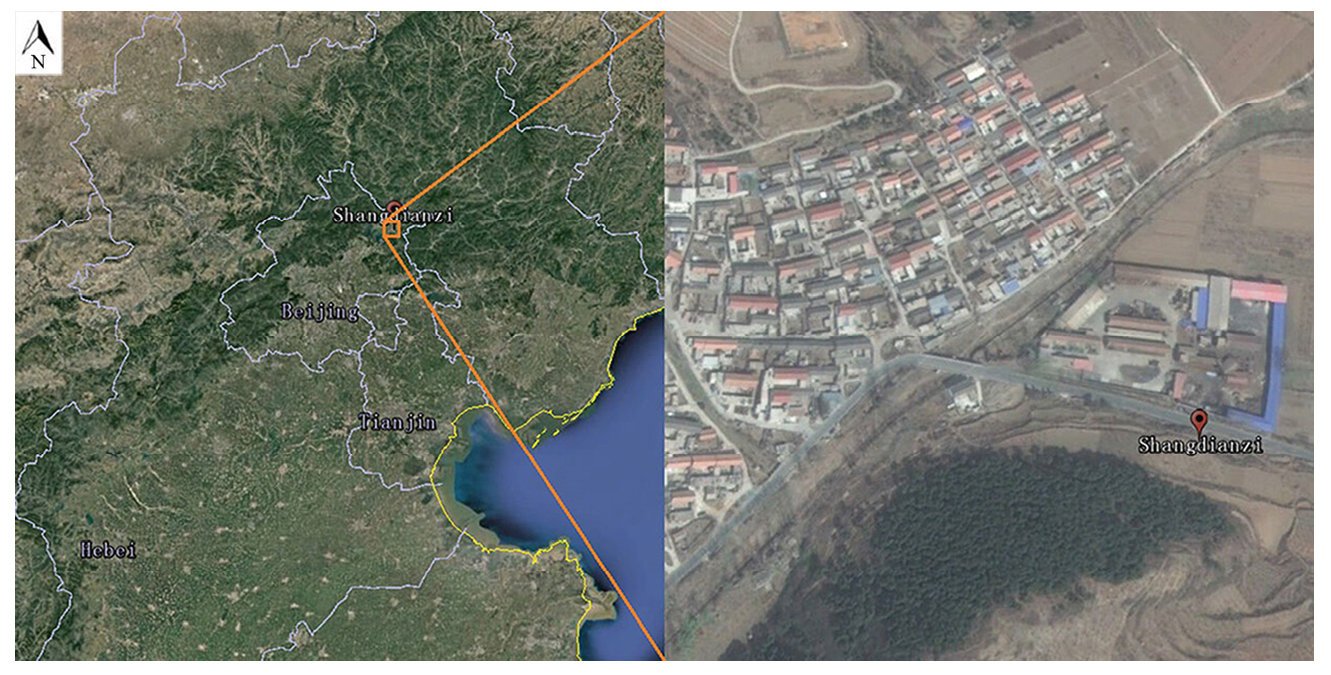
2.1. Study Site

As shown in Figure 1, the SDZ (40°39’ N, 117°07’ E, 293.9 m a.s.l.) site selected for applying the proposed methodology is located in the northern part of NCP and is 100 km northeast of the urban area of Beijing. It is one of the regional Global Atmosphere Watch (GAW) stations in China. There are no densely populated and industrial areas within a distance of 30 km around the station, so the atmospheric pollution level at SDZ station represents the background concentration of atmospheric pollutants in the economically developed regions of north China. The prevailing winds at SDZ are influenced by the valley topography and are from east-northeast and west-southwest. When southwesterly winds arise, the polluted air masses from urban areas and satellite towns of Beijing can be transported to SDZ while relatively clean air masses arrive from other wind directions. There has been detailed information regarding SDZ site presented in previous studies [34,35].

2.2. Data Preparation

The data used in this paper have the time frame of 14 to 23 January 2010 during which a regional haze episode occurred in the Beijing, Tianjin and Hebei Provinces (BTH) area in the NCP from 16 to 19 January 2010. At SDZ station, concentrations of CO, NO₂, O₃, SO₂ and PM_2.5 were observed by a TE48C CO analyzer, TE 42CTL NO_X analyzer, TE49C O₃ analyzer, TE43C SO₂ analyzer and a tapered element oscillating microbalance (TEOM 1400a), respectively. An automatic weather station installed at the SDZ meteorological station measured the hourly meteorological data including T, RH, WS, WD, Pre and Vis. The AOD retrieved with the lidar observation was also presented in the study of Zhao et al. [36]. The meteorological variables and air pollutants except PM_2.5 as well as AOD constitute the predictors and the PM_2.5 is the predictand. The entire data table of the predictors and predictand consists of 240 h of measurements and was uploaded as non-published material during the submission process. Considering that the values of AOD were mostly missed on 19 January due to the presence of cumulus clouds at the top of the planetary boundary layer (PBL), the rows from 13:00 18 January to 23:00 19 January were eliminated. The hourly measurements from 1:00 23 January to 23:00 23 January 2010 were also deleted owing to the missing corresponding predictand values. Finally, only 182 h of measurements were chosen for the present study. The units of most variables are summarized in

Table 1. Units of variables measured at SDZ.

Variables	T	RH	WS	WD	Pre	Vis	CO	NO2	O3	SO2	PM2.5
Units	°C	%	m/s	°	hPa	km	ppm	ppb	ppb	ppb	μg/m3

and the AOD is a non unit variable.

3. Theory and Methodology

PM_2.5 concentrations are affected by emission sources, meteorological conditions and topographical characteristics of the area under study, which makes estimating the PM_2.5 distribution difficult. In order to model the hourly concentrations of PM_2.5 at SDZ precisely, the SOG-SASOFNN was developed to forecast the PM_2.5 concentrations of the next 24 h employing the current hour values of the dominating parameters extracted by PCA.

3.1. Principal Component Analysis

PCA is a classical statistical technique that analyzes the covariance structure of multivariate variables and has been successfully applied for several tasks in AQ domain [37,38]. In this paper, PCA was used to provide the interdependencies of the data measured at SDZ station. PCA selected the dominating variables having the greatest impact on PM_2.5 in the following steps:

• Let 182 × 11 data matrix $\mathbf{X}=[{\mathbf{x}}_1,{\mathbf{x}}_2,\mathrm{...},{\mathbf{x}}_{11}]$ denotes the 182 h of measurements of predictors and ${\mathbf{x}}_1,{\mathbf{x}}_2,...,{\mathbf{x}}_{11}$ are 182 × 1 data vectors of T, RH, WS, WD, Pre, Vis, AOD, CO, NO₂, O₃ and SO₂, respectively. The data matrix should be transformed into a standardized form:

  $$\mathbf{Z}={(z_{ij})}_{182\times 11}={\left(\frac{x_{ij}-{\overline{\mathbf{x}}}_j}{{\delta }_j}\right)}_{182\times 11},i=1,2,...,182;j=1,2,...,11$$

  (1)

  where $\mathbf{Z}$ is the standardized data matrix generated from $\mathbf{X}$; $x_{ij}$ and $z_{ij}$ are the values of predictor j in sample i before and after the standardization; and ${\overline{\mathbf{x}}}_j$ and ${\delta }_j$ are the arithmetic mean value and the standard deviation for predictor j, respectively.
• Calculate the correlation coefficient matrix using Equation (2):

  $$\mathbf{R}=\frac{1}{182}{\mathbf{Z}}^T\mathbf{Z}$$

  (2)
• Compute the eigenvalues ${\lambda }_1,{\lambda }_2,...,{\lambda }_{11}$ and the corresponding eigenvectors ${\mathbf{\gamma }}_1,{\mathbf{\gamma }}_2,...,{\mathbf{\gamma }}_{11}$ of 11 × 11 correlation matrix $\mathbf{R}$.
• Reorder the eigenvalues in descending order to bring ${\lambda }_1^{\text{'}}>{\lambda }_2^{\text{'}}>...>{\lambda }_{11}^{\text{'}}$ and readjust the eigenvectors as ${\mathbf{\gamma }}_1^{\text{'}},{\mathbf{\gamma }}_2^{\text{'}},...,{\mathbf{\gamma }}_{11}^{\text{'}}$ accordingly.
• Obtain the unit orthogonal eigenvectors ${\mathbf{\rho }}_1,{\mathbf{\rho }}_2,...,{\mathbf{\rho }}_{11}$ using the Schmidt orthogonal method on ${\mathbf{\gamma }}_1^{\text{'}},{\mathbf{\gamma }}_2^{\text{'}},...,{\mathbf{\gamma }}_{11}^{\text{'}}$.
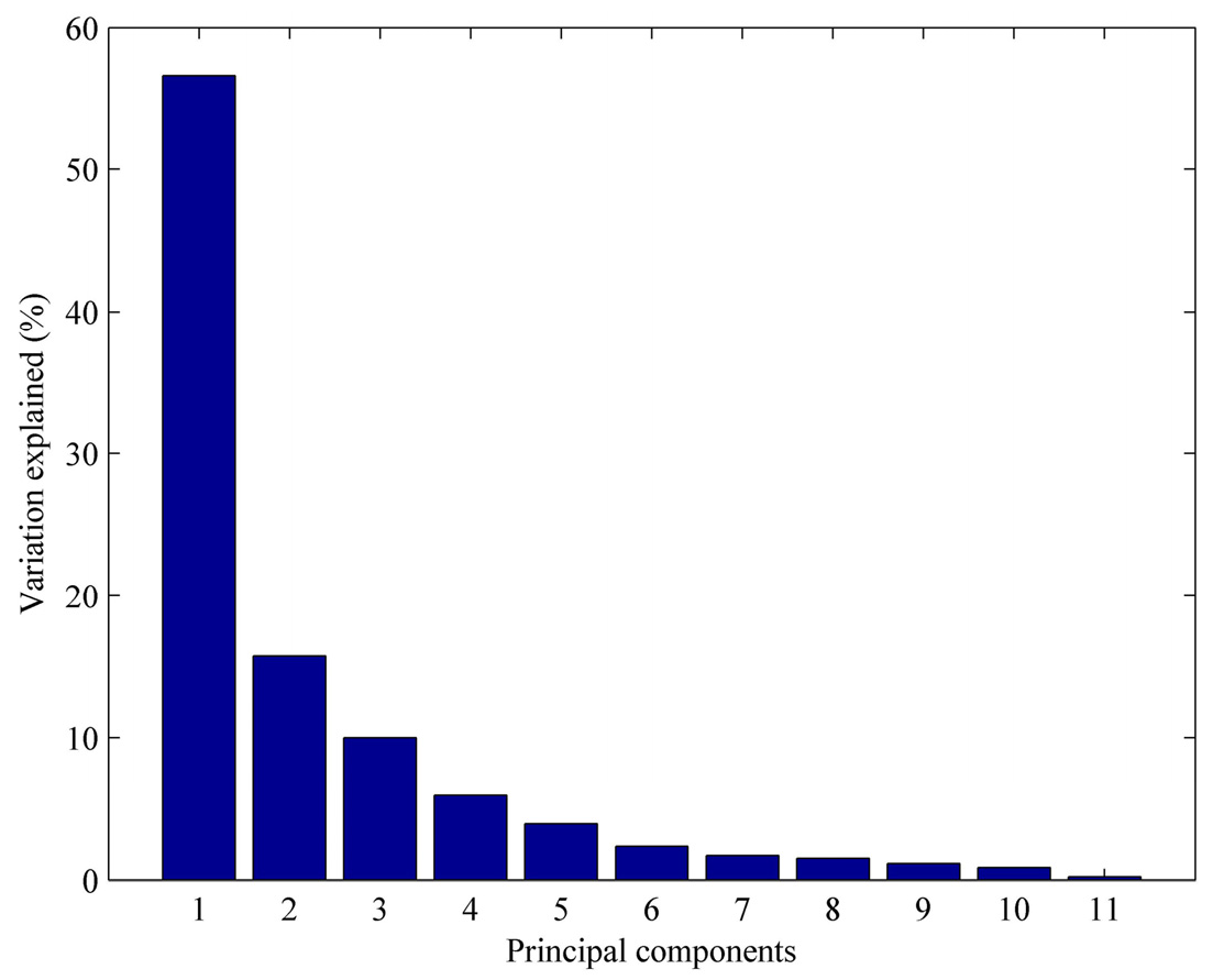
• Calculate the cumulative contribution rate ${\theta }_1,{\theta }_2,...,{\theta }_{11}$ of the eigenvalues ${\lambda }_1^{\text{'}},{\lambda }_2^{\text{'}},...,{\lambda }_{11}^{\text{'}}$ and $\alpha$ variables will be extracted if ${\theta }_{\alpha }\ge \theta$ where $\theta$ is the preset extraction efficiency.
• The data of the dominating variables is acquired by computing the projection of $\mathbf{Z}$ on the extracted unit orthogonal eigenvectors using Equation (3):

  $$\mathbf{Y}=\mathbf{Z}\mathbf{\rho }$$

  (3)

  where $\mathbf{\rho }=[{\mathbf{\rho }}_1,{\mathbf{\rho }}_2,...,{\mathbf{\rho }}_{\alpha }]$.

3.2. Sensitivity Analysis Based Self-Organizing Fuzzy Neural Network with Second Order Gradient Algorithm

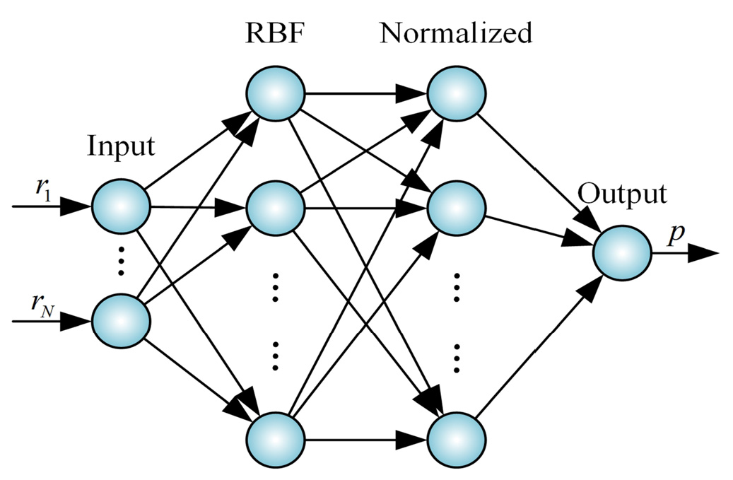
3.2.1. Architecture of the Proposed Model

The SOG-SASOFNN used to search a suitable nonlinear mapping between the dominating variables and the hourly concentrations of PM_2.5 in the present study is based on radial basis function (RBF) neurons. As shown in Figure 2, the initial architecture of the SOG-SASOFNN has four layers, the input layer, the RBF layer, the normalized layer and the output layer.

Mathematically, each layer in the initial SOG-SASOFNN is described as follows:

• Input layer: There are N neurons in this layer and the output value of the ith neuron can be expressed as follows:

  $$u_i=r_i,i=1,2,...,N$$

  (4)

  where $\mathbf{r}=[r_1,r_2,...,r_N]$ represents the dominating variables extracted from the predictors through PCA method.
• RBF layer: The Gaussian membership functions (MFs) of every of RBF neurons in this layer is selected to deal with the input variables. Each RBF neuron represents an if-part of a fuzzy rule, and the outputs of RBF neurons are calculated in the following manner:

  $${\psi }_j=\text{exp}(-{\displaystyle {\sum }_{i=1}^N({(u_i-c_{ij})}^2/2{\sigma }_{ij}^2})),i=1,2,...,N;j=1,2,...,M$$

  (5)

  where ${\psi }_j$ is the output of the jth RBF neuron; $c_{ij}$ and ${\sigma }_{ij}$ are the center and width of the ith membership function (MF) in the jth neuron, respectively; and M is the total number of neurons in this layer.
• Normalized layer: The number of the neurons in the normalized layer is the same as that in the RBF layer. The output values of nodes in this layer are given as follows:

  $$v_l=\frac{\text{exp}(-{\displaystyle {\sum }_{i=1}^N({(u_i-c_{il})}^2/2{\sigma }_{il}^2}))}{{\displaystyle {\sum }_{j=1}^{M}exp(-{\displaystyle {\sum }_{i=1}^N({(u_i-c_{ij})}^2/2{\sigma }_{ij}^2}))}},i=1,2,...,N;j=1,2,...,M;l=1,2,...,M$$

  (6)

  where $v_l$ is the lth output value in the normalized layer.
• Output layer: There is only one neuron in this layer, in which of the output represents the PM_2.5 concentration that can be clarified through the gravity method given as follows:

  $$p=\frac{{\displaystyle {\sum }_{l=1}^M{w}_l\text{exp}(-{\displaystyle {\sum }_{i=1}^N({(u_i-c_{il})}^2/2{\sigma }_{il}^2}))}}{{\displaystyle {\sum }_{j=1}^M\text{exp}(-{\displaystyle {\sum }_{i=1}^N({(u_i-c_{ij})}^2/2{\sigma }_{ij}^2}))}},i=1,2,...,N;j=1,2,...,M;l=1,2,...,M$$

  (7)

  where $w_l$ is the weight connecting the lth neuron in the normalized layer and the neuron in the output layer.

Moreover, 130 h of measurements of dominating variables and PM_2.5 from the total 182 rows of data were randomly selected as training set of the SOG-SASOFNN, and the remaining data were regarded as test set. Thus, both the training set and the test set cover measurements from haze period (from 16 to 19 January 2010) and non-haze days (all other days from 14 to 23 January 2010). All data sets were normalized to the range of [0, 1] by linear scaling. Once the structure and the parameters of the SOG-SASOFNN were optimized through training, this optimized function was used to make prediction on the test data. The statistical parameters index of agreement (IA), coefficient of determination (R²), normalized mean bias (NMB), normalized mean gross error (NMGE), root mean square error (RMSE) and mean bias (MB) were used to assess the models performances between observed and predicted concentrations of PM_2.5 [39,40]. The definitions of these statistical parameters are shown in

Table 2. Definitions of statistical parameters used for assessing the models performances.

Statistical Parameter	Description	Mathematical Function
IA	Expresses the difference between predicted and observed values	$IA=1-\frac{{\displaystyle {\sum }_{i=1}^n{\left|p_i-o_i\right|}^2}}{{\displaystyle {\sum }_{i=1}^n{\left(\left|p_i-\overline{o}\right|+\left|o_i-\overline{o}\right|\right)}^2}}$
R2	A measure of linear relationship between predicted and observed values	$R^2=\frac{{\left({\displaystyle {\sum }_{i=1}^n\left(p_i-\overline{p}\right)\left(o_i-\overline{o}\right)}\right)}^2}{{{\displaystyle {\sum }_{i=1}^n\left(p_i-\overline{p}\right)}}^2{{\displaystyle {\sum }_{i=1}^n\left(o_i-\overline{o}\right)}}^2}$
NMB	Indicates over or under estimation of the model	$NMB=\frac{{\displaystyle {\sum }_{i=1}^n\left(p_i-o_i\right)}}{{\displaystyle {\sum }_{i=1}^n{o}_i}}$
NMGE	Indicates mean error regardless of it is over or under estimation	$NMGE=\frac{{\displaystyle {\sum }_{i=1}^n\left|p_i-o_i\right|}}{{\displaystyle {\sum }_{i=1}^n{o}_i}}$
RMSE	Provides an overall measure of how close predicted values and observed values are	$RMSE=\sqrt{\frac{{\displaystyle {\sum }_{i=1}^n{\left(p_i-o_i\right)}^2}}{n}}$
MB	Measure of model bias	$MB=\frac{{\displaystyle {\sum }_{i=1}^n\left(p_i-o_i\right)}}{n}$

, where $p_i$ refers to the ith predicted value and $o_i$ to the ith observed one for a total of n observations; and $\overline{p}$ and $\overline{o}$ are the averages of predicted values and observed values, respectively. Note that the normalized mean error (NME) used in the study of Yu et al. [13] and the NMGE described in our manuscript are equal in formula [39].

3.2.2. Sensitivity Analysis Method

In this present study, the SA was used to adjust the structure of the SOG-SASOFNN during training phase to understand the dynamic process that produces PM_2.5 from pollution sources. SA is a method that evaluates the dependency of the system output on the input factors. The contribution of the output of each neuron in the normalized layer to the output of the SOG-SASOFNN was measured by global SA method in this paper. The measurement is based on the Fourier decomposition of variance [41,42]. The input parameters used for performing SA are the outputs of the normalized neurons expressed as $\mathbf{v}={[v_1,v_2,...,v_M]}^T$. The SOG-SASOFNN output representing the PM_2.5 concentration can be described as follows:

$$p=f(v_1,v_2,...,v_M)$$

(8)

The first order sensitivity index of the output of the hth normalized neuron to the SOG-SASOFNN output is given by:

$$S_h=\frac{{Var}_{v_h}[E(p|v_h={\beta }_h)]}{Var(p)},h=1,2,...,M$$

(9)

where $E(p|v_h={\beta }_h)$ denotes the expected value of p under the condition that the value of $v_h$ is equal to ${\beta }_h$ and the variance ${Var}_{v_h}$ takes over all the possible values of $v_h$. $Var(p)$ represents the variance of p.

If the range of the input factor $v_h$ is $[a_h,b_h]$, it can be written as:

$$v_h(s)=\frac{b_h+a_h}{2}+\frac{b_h-a_h}{\pi }\text{arcsin}(\text{sin}({\omega }_{h}s)),h=1,2,...,M$$

(10)

where ${\omega }_h$ is the fundamental frequency of $v_h$. The equation allows each factor to oscillate in a given range periodically as the scalar variable s varying in the range [−∞, ∞]. The M-factor model in Equation (8) can be described in the frequency domain using the following relationship:

$$f(s)=f(v_1(s),v_2(s),...,v_M(s))$$

(11)

The expanded Fourier series of $f(s)$ is given by:

$$f(s)={\displaystyle {\sum }_{\omega =-\infty }^{\infty }(A_{\omega }\text{cos}(\omega s)+B_{\omega }\text{sin}(\omega s))}$$

(12)

where the Fourier coefficients at frequency $\omega$ are defined as:

$$\begin{array}{l}{A}_{\omega }=\frac{1}{2\pi }{\displaystyle {\int }_{-\pi }^{\pi }f}(s)\text{cos}(\omega s)ds\\ B_{\omega }=\frac{1}{2\pi }{\displaystyle {\int }_{-\pi }^{\pi }f}(s)\text{sin}(\omega s)ds\end{array}$$

(13)

where s is on the range of $[-\pi ,\pi ]$. The variance of p is calculated by the Fourier translation:

$$Var(p)=2{\displaystyle {\sum }_{\omega =1}^{\infty }(A_{\omega }^2+B_{\omega }^2)}$$

(14)

The portion of the variance of p caused by $v_h$ alone is expressed as:

$${Var}_{v_h}[E(p|v_h={\beta }_h)]=2{\displaystyle {\sum }_{m=1}^{\infty }(A_{m{\omega }_h}^2+B_{m{\omega }_h}^2)},h=1,2,...,M$$

(15)

where $A_{m{\omega }_h}$ and $B_{m{\omega }_h}$ denote the Fourier coefficients for the fundamental frequency of $v_h$ and its higher harmonics $m{\omega }_h$. Consequently, the expansion of the first order sensitivity index is given by:

$$S_h=\frac{{\displaystyle {\sum }_{m=1}^{\infty }(A_{m{\omega }_h}^2+B_{m{\omega }_h}^2)}}{{\displaystyle {\sum }_{\omega =1}^{\infty }(A_{\omega }^2+B_{\omega }^2)}},h=1,2,...,M$$

(16)

Because the Fourier amplitude decreases as the frequency goes up, it is expected that the high order Fourier coefficients have negligible influence on the variation of the model output. Thus, the first order sensitivity index is approximated as:

$$S_h\approx \frac{{\displaystyle {\sum }_{m=1}^P(A_{m{\omega }_h}^2+B_{m{\omega }_h}^2)}}{{\displaystyle {\sum }_{\omega =1}^{P{\omega }_{\text{max}}}(A_{\omega }^2+B_{\omega }^2)}},h=1,2,...,M$$

(17)

where P is called the interference factor, which is usually set to 4 or 6 in the SA community, and ${\omega }_{max}$ is the maximum value of the fundamental frequencies of all input factors.

In order to obtain the total sensitivity index, set ${\omega }_h=2P\text{max}({\omega }_{~h})$ where $\text{max}({\omega }_{~h})$ is the highest fundamental frequency of the remaining set of factors $v_{~h}$ (all the factors except the hth factor) to ensure that the frequencies generated by all interactions involving $v_h$ will not interfere with the frequencies induced by the nonlinear effect involving $v_{~h}$ alone. Then, the estimation of the total sensitivity index ${\text{SW}}_h$ is as follows:

$${\text{SW}}_h=\frac{{\displaystyle {\sum }_{\omega =P\text{max}({\omega }_{~h})+1}^{P{\omega }_h}(A_{\omega }^2+B_{\omega }^2)}}{{\displaystyle {\sum }_{\omega =1}^{P{\omega }_h}(A_{\omega }^2+B_{\omega }^2)}},h=1,2,...,M$$

(18)

Because the outputs of neurons in the normalized layer are independent with each other, the total sensitivity index ${\text{SW}}_h$ can be acquired by the calculation of Fourier amplitude at fundamental frequency barely and is simplified as follows:

$${\text{SW}}_h=\frac{A_{{\omega }_h}^2+B_{{\omega }_h}^2}{{\displaystyle {\sum }_{j=1}^M(A_{{\omega }_j}^2+B_{{\omega }_j}^2)}},h=1,2,...,M$$

(19)

Based on the analysis above, the standardized total sensitivity index ${\text{ST}}_h$ of the output of the hth neuron in the normalized layer over the SOG-SASOFNN output is computed as follows:

$${\text{ST}}_h=\frac{{\text{SW}}_h}{{\displaystyle {\sum }_{j=1}^M{\text{SW}}_j}},h=1,2,...,M$$

(20)

3.2.3. Second Order Gradient Algorithm

To further improve the accuracy of prediction of hourly PM_2.5 distribution, the parameter-learning phase of the SOG-SASOFNN was performed through the SOG algorithm proposed in the study of Xie et al. [32]. The SOG algorithm does not suffer from enormous Jacobian matrix and its side effects when training data are huge. All parameters such as centers, widths and weights of the SOG-SASOFNN adjusted by the SOG algorithm are expressed as follows:

$$\mathbf{\Phi }(t)=[c_{11}(t),...,c_{NM}(t),{\sigma }_{11}(t),...,{\sigma }_{NM}(t),w_1(t),...,w_M(t)]$$

(21)

where $t$ is the current time (or training step). $\mathbf{\Phi }(t)$ is the parameter vector of the SOG-SASOFNN at time t.

Following the Levenberg–Marquardt (LM) algorithm [31], the update rule is given by:

$$\mathbf{\Phi }(t+1)=\mathbf{\Phi }(t)+{(\mathbf{Q}(t)+\mu (t)\mathbf{I})}^{-1}\mathbf{g}(t)$$

(22)

where $\mathbf{Q}(t)$ is the quasi Hessian matrix computed as the sum of the sub matrix ${\mathbf{q}}_k(t)$ for the kth training pattern:

$$\mathbf{Q}(t)={\displaystyle {\sum }_{k=1}^K{\mathbf{q}}_k(t)},{\mathbf{q}}_k(t)={\mathbf{j}}_k^T(t){\mathbf{j}}_k(t)$$

(23)

and the gradient vector $\mathbf{g}(t)$ is calculated as the sum of the sub vector ${\mathbf{\eta }}_k(t)$ for the kth training pattern:

$$\mathbf{g}(t)={\displaystyle {\sum }_{k=1}^K{\mathbf{\eta }}_k(t)},{\mathbf{\eta }}_k(t)={\mathbf{j}}_k^T(t)e_k(t)$$

(24)

where K is the amount of rows of training pattern with value of 130. ${\mathbf{j}}_k(t)$ is one of the rows of Jacobian matrix for pattern k described as follows:

$${\mathbf{j}}_k(t)=[\frac{\partial e_k(t)}{\partial c_{11}(t)},...,\frac{\partial e_k(t)}{\partial c_{NM}(t)},\frac{\partial e_k(t)}{\partial {\sigma }_{11}(t)},...,\frac{\partial e_k(t)}{\partial {\sigma }_{NM}(t)},\frac{\partial e_k(t)}{\partial w_1(t)},...,\frac{\partial e_k(t)}{\partial w_M(t)}]$$

(25)

where $e_k(t)$ is the error calculated by:

$$e_k(t)=o_k(t)-p_k(t)$$

(26)

where $o_k(t)$ and $p_k(t)$ are the observed output and predicted output when the kth training pattern is presented at time t, respectively.

Be aware that the combination coefficient $\mu (t)=\Vert \mathbf{g}(t)\Vert$ and I is the identity matrix.

3.2.4. Design of the Second Order Sensitivity Analysis Based Self-Organizing Fuzzy Neural Network

The SOG-SASOFNN applied to forecast the hourly concentrations of PM_2.5 for the next 24 h at SDZ from 14 to 23 January was trained with SA method and SOG algorithm. The computation procedure of the SOG-SASOFNN is described as follows:

• Initialization of the SOG-SASOFNN: The initial SOG-SASOFNN is with random number of neurons in the normalized layer and the inputs of the SOG-SASOFNN are dominating variables selected through PCA method. There is one neuron in the output layer in which of the output represents the PM_2.5 concentration. The parameters such as centers, widths, and weights of the SOG-SASOFNN are initially distributed on the random range of [0, 1].
• Parameter learning: Adjust the parameters of the SOG-SASOFNN using Equation (22) with all training set for several training steps.
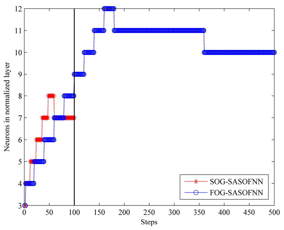
• Growing phase: After some time ($\Theta$) steps, calculate the standardized total sensitivity index of output of each normalized neuron to the network output using Equation (20). The hth normalized neuron is overactive and will be spilt into two new normalized neurons if ${\text{ST}}_h$ is larger than ${\epsilon }_1$. In order to guarantee the convergence, the outputs of the SOG-SASOFNN before and after the structure has been adjusted must be identical and the initial parameters of the two new normalized neurons are set as follows:

  $$\begin{array}{l}{\mathbf{c}}_{•new1}={\mathbf{c}}_{•new2}={\mathbf{c}}_{•h}(t)\\ {\mathbf{\sigma }}_{•new1}={\mathbf{\sigma }}_{•new2}={\mathbf{\sigma }}_{•h}(t)\\ w_{new1}=\tau w_h(t),w_{new2}=(1-\tau )w_h(t)\end{array}$$

  (27)

  where new1 and new2 denote the two new normalized neurons. ${\mathbf{c}}_{•new1}$, ${\mathbf{\sigma }}_{•new1}$ and $w_{new1}$ are the center vector, width vector and weight of neuron new1, respectively. ${\mathbf{c}}_{•new2}$, ${\mathbf{\sigma }}_{•new2}$ and $w_{new2}$ are the center vector, width vector and weight of neuron new2, respectively. ${\mathbf{c}}_{•h}(t)$, ${\mathbf{\sigma }}_{•h}(t)$ and $w_h(t)$ are the center vector, width vector and weight of the hth normalized neuron before the structure has been adjusted at step t, respectively. $\tau$ is a random number which is distributed in the range of [0, 1].
• Pruning phase: The hth normalized neuron is useless and will be pruned if ${\text{ST}}_h$ is less than ${\epsilon }_2$. To reduce the fluctuation of the output of the network, the parameters of the nearest neuron are compensated as:

  $$\begin{array}{l}{\mathbf{c}}_{•nea}={\mathbf{c}}_{•nea}(t)\\ {\mathbf{\sigma }}_{•nea}={\mathbf{\sigma }}_{•nea}(t)\\ w_{nea}=w_{nea}(t)+w_h(t)v_h(t)/v_{nea}(t)\end{array}$$

  (28)

  where nea is the normalized neuron with the minimum Euclidean distance to the hth normalized neuron and ${\text{ST}}_{nea}\ge {\epsilon }_2$. ${\mathbf{c}}_{•nea}$, ${\mathbf{\sigma }}_{•nea}$ and $w_{nea}$ are the center vector, width vector and weight of neuron nea after pruning at step t, respectively. ${\mathbf{c}}_{•nea}(t)$, ${\mathbf{\sigma }}_{•nea}(t)$ and $w_{nea}(t)$ are the center vector, width vector and weight of neuron nea before pruning at step t, respectively. $w_h(t)$ is the weight of the hth normalized neuron before pruning when training to step t. $v_h(t)$ and $v_{nea}(t)$ are the output of the hth normalized neuron and neuron nea before pruning when training to step t, respectively.
• Relearning of parameters: Turn the algorithm to procedure 2 to make the parameters under relearning applying Equation (22). The training process terminates when the process achieves the expected training RMSE E_d or reaches the pre-set running step R_max.
• Test stage: Once the SOG-SASOFNN is optimized by the training set, this optimized nonlinear function is used to make prediction on the test data.

4. Results and Discussion

In this paper, the dominating variables most correlated to PM_2.5 were firstly selected by the PCA method using the data measured at SDZ from 14 to 23 January 2010. Then, the SOG-SASOFNN was developed to forecast the PM_2.5 concentrations of the next 24 h with the current hour values of dominating variables at SDZ during the studied period. Finally, the prediction performance of the SOG-SASOFNN was compared with that of the FOG-SASOFNN and the ESN as well as with the performance of the Eta-CMAQ in modeling the hourly PM_2.5 concentrations at the rural sites over the eastern United States from 15 July to 19 August 2004 to verify the effectiveness of using SOG-SASOFNN to estimate the hourly PM_2.5 distribution at SDZ.

4.1. Variation of PM_2.5 Concentrations with Meteorological Conditions and Aerosol Optical Depth at SDZ

A regional haze episode occurred in the BTH region in the NCP from 16 to 19 January 2010 and was caused by a surface high-pressure system from 16 to 18 January 2010 and a low-pressure system on 20 January, which was unfavorable for the dispersion of pollutants. Figure 3 shows the measured temporal variation of PM_2.5 and the modeled results for the SOG-SASOFNN, the FOG-SASOFNN and the ESN. According to Figure 3, the PM_2.5 concentrations at SDZ during the haze period are much higher than that in non-haze days although there were no significant pollution sources within 30 km of the site, mainly owing to the regional transportation from the southern urban area. The surface wind at SDZ turning from east-northeast to southwest in the afternoon of 18 January, which carried pollutants to this area, led to the highest aerosol loading on 19 January. During the haze period, the T increased continuously day by day and the RH remained high at SDZ. PM_2.5 concentrations in the haze episode were also high enough to extinct the light and the low Vis recorded in daytime indicated the haze phenomenon. Similar to the variation of PM_2.5 concentration, the AOD began to increase on 16 January and increased significantly in the afternoon of 18 January to reach its maxima on 19 January. Under the Mongolia anticyclone with strong northerly wind, the haze episode was finally terminated on 20 January. Evidently, the variation of the PM_2.5 concentrations at SDZ station relies seriously on the meteorological variables and is closely related to the AOD. Besides, we could find that the modeled result of the SOG-SASOFNN is more reasonable than that of the FOG-SASOFNN and the ESN.

4.2. Dominating Variables Selected by Principal Component Analysis

PCA was performed to extract the dominating factors for PM_2.5 among the predictors at SDZ station. The percentages of process variance explained by principal components (PCs) defined as $\text{PCs}=[\text{PCs}1,\text{PCs}2,...,\text{PCs}11]$ are shown in Figure 4 and

Table 3. Percent and additive percent of process variance caused by PCs.

PCs	1	2	3	4	5	6	7	8	9	10	11
Percent (%)	56.55	15.71	10.00	5.98	4.01	2.34	1.71	1.50	1.13	0.86	0.21
Additive percent (%)	56.55	72.26	82.26	88.24	92.25	94.59	96.30	97.80	98.93	99.79	100

.

As shown in Table 3, over 90% of the variation within the data can be explained by the former five PCs, and the most important variables (dominating variables) for the former five PCs are RH, Pre, AOD, WS and WD according to the coefficients of the selected PCs given in Equation (29):

$$\begin{array}{l}\text{PCs}1=[-0.06\hspace{0.17em}0.07\hspace{0.17em}0.24\hspace{0.17em}0.06-0.04-0.27-0.42-0.22-0.31\hspace{0.17em}0.20-0.11]\\ \text{PCs}2=[0.33-0.10-0.34-0.05\hspace{0.17em}0.49\hspace{0.17em}0.04-0.34-0.38\hspace{0.17em}0.25-0.40\hspace{0.17em}0.16]\\ \text{PCs}3=[-0.28\hspace{0.17em}0.39-0.16\hspace{0.17em}0.15\hspace{0.17em}0.49\hspace{0.17em}0.18\hspace{0.17em}0.61-0.25-0.04\hspace{0.17em}0.09-0.04]\\ \text{PCs}4=[0.12-0.13\hspace{0.17em}0.80-0.36\hspace{0.17em}0.42\hspace{0.17em}0.07\hspace{0.17em}0.08-0.01-0.06\hspace{0.17em}0.03\hspace{0.17em}0.01]\\ \text{PCs}5=[-0.20-0.38-0.27\hspace{0.17em}0.77\hspace{0.17em}0.15-0.25-0.11-0.22-0.06-0.03\hspace{0.17em}0.01]\end{array}$$

(29)

It could be noted that the dominating variables (RH, Pre, AOD, WS and WD) extracted through PCA are consistent with the characteristics of PM_2.5 at SDZ where the PM_2.5 concentrations are severely correlated to the meteorological parameters and the AOD.

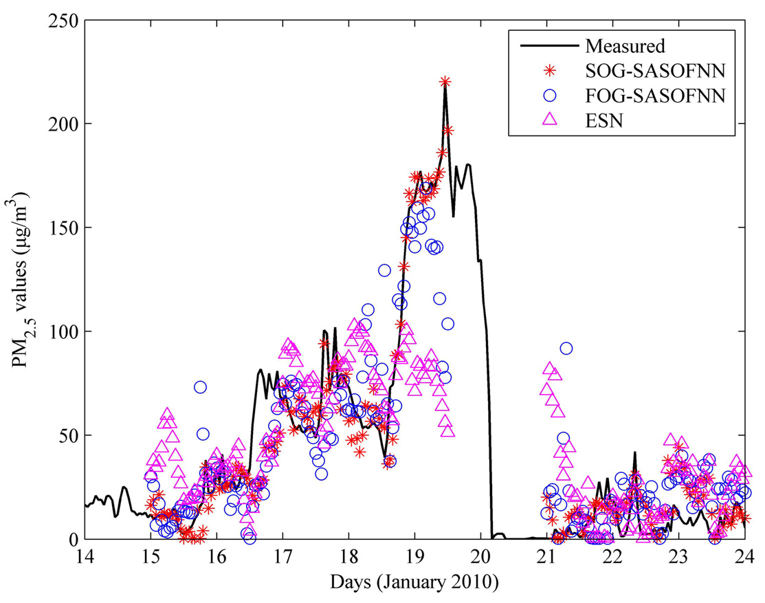
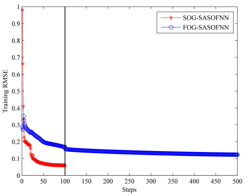
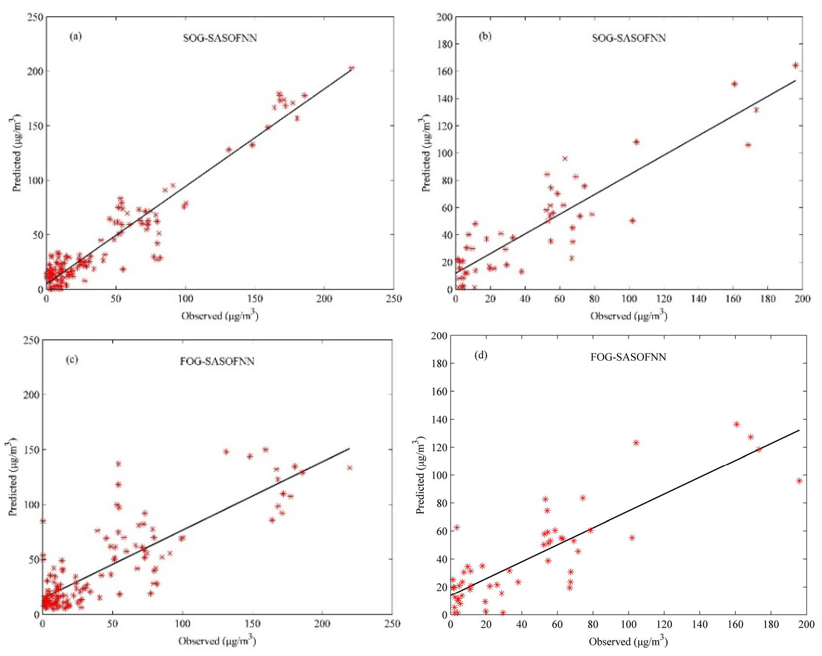
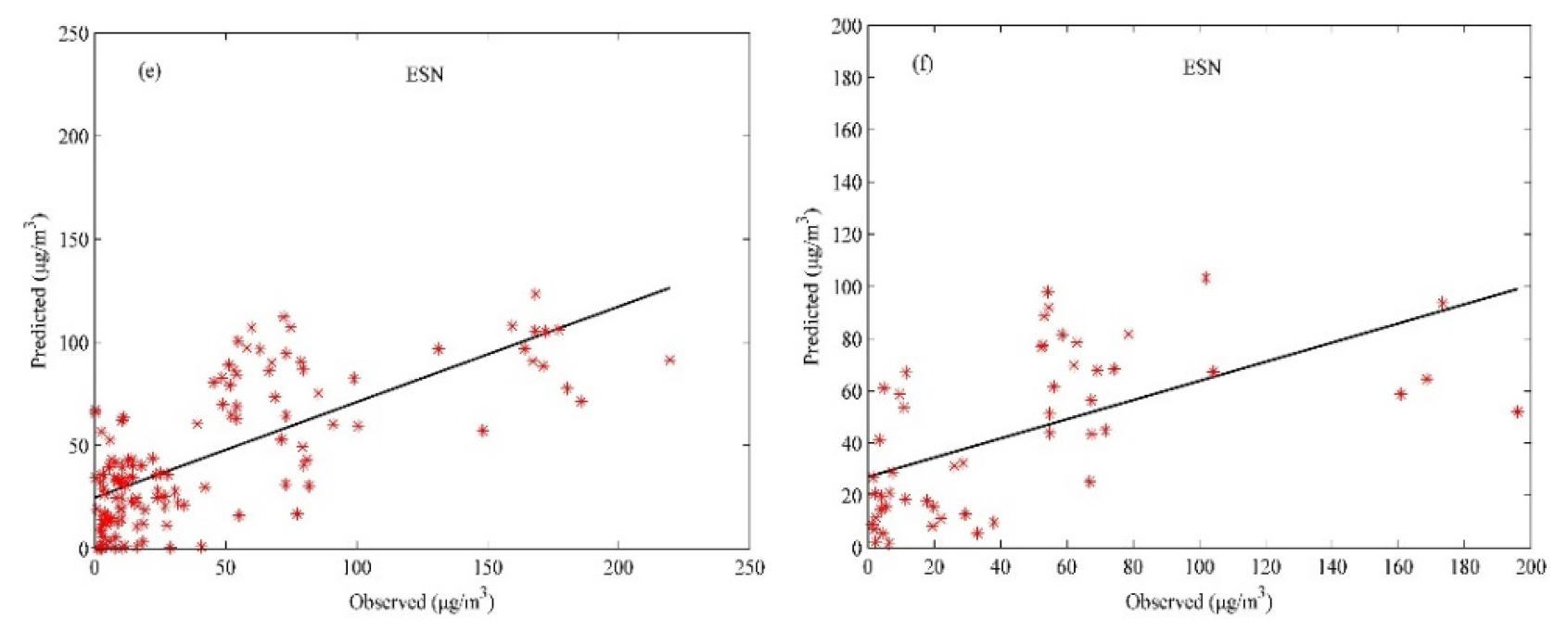
4.3. Modeling: Training and Validation

The SOG-SASOFNN was developed to predict the hourly PM_2.5 concentrations 24 h ahead at SDZ along with the FOG-SASOFNN and the ESN in the present study. For SOG-SASOFNN, the first 130 h of 182 rows of randomized and normalized measurements of dominating variables and PM_2.5 were used as training set and the rest 52 observations were taken as test set. The input layer of the SOG-SASOFNN consisted of five parameters containing RH, Pre, AOD, WS and WD selected by PCA. There were three neurons in the normalized layer before the input data have been loaded. The parameters (centers, widths and weights) of the SOG-SASOFNN were initialized on the random range of [0, 1]. The structure of the SOG-SASOFNN was adjusted based on the contribution of the output of each normalized neuron to the output of network measured by global SA method. The parameter-learning phase was performed using Equation (22). The network was trained for 100 steps with $\Theta =10$ unless the training RMSE was less than 0.01. The input parameters of the FOG-SASOFNN and the ESN were the same as that of the SOG-SASOFNN. The FOG-SASOFNN was optimized after it was trained for 500 steps or the training RMSE was less than 0.01. The weight-learning process for the ESN was implemented applying linear regression equation [11]. The description and the evaluation of the PM_2.5 forecasts over the eastern United States using the Eta-CMAQ model was presented in detail in the study of Yu et al. [13].

The change of the training RMSE of the SOG-SASOFNN and the FOG-SASOFNN during learning phase is shown in Figure 5. The growing and pruning process of the neurons in the normalized layer of the SOG-SASOFNN and the FOG-SASOFNN for the training period has been shown in Figure 6. In Figure 5 and Figure 6, we could find that the SOG-SASOFNN converges with lower training RMSE and more compact structure under much less training steps compared to the FOG-SASOFNN.

Figure 7 shows the scatter plots between the observed and predicted concentrations of PM_2.5 during training phase and test phase for the SOG-SASOFNN, the FOG-SASOFNN and the ESN. As can be seen in Figure 7, the SOG-SASOFNN possesses stronger learning ability and better generalization performance compared to the FOG-SASOFNN and the ESN.

The models’ performances were evaluated by the calculation of several statistical parameters indexes described in Table 2. The statistical performances for the SOG-SASOFNN, the FOG-SASOFNN, the ESN and the Eta-CMAQ are given in

Table 4. Statistical performances of SOG-SASOFNN, FOG-SASOFNN, ESN and Eta-Community Multiscale Air Quality (Eta-CMAQ) model.

Statistical Parameter	Ideal Value	SOG-SASOFNN		FOG-SASOFNN		ESN		Eta-CMAQ
		Training	Test	Training	Test	Training	Test
IA	1	0.97	0.95	0.91	0.86	0.80	0.70	~
R2	1	0.89	0.84	0.72	0.70	0.51	0.30	0.22 *
NMB	0	−0.01	−0.05	−0.17	−0.23	−0.26	0.31	−0.32 *
NMGE	0	0.25	0.37	0.42	0.43	0.52	0.57	0.51*
RMSE (μg/m3)	0	13.56	17.90	26,84	29.31	35.35	39.79	11.6 *
MB (μg/m3)	0	−0.16	−1.86	−2.01	−3.6	−5.61	6.33	−5.2 *

~ The value does not shown in original paper; * The results are the same as the original paper.

. It can be found that the values of R², NMB, NMGE and MB for the SOG-SASOFNN in both training phase and test phase are closer to their corresponding ideal values contrasted to that for the FOG-SASOFNN, the ESN as well as the Eta-CMAQ. The training RMSE and test RMSE of the SOG-SASOFNN are larger than the Eta-CMAQ RMSE, which may be due to the data used in our paper covers wider PM_2.5 concentrations scope compared with the data for the Eta-CMAQ. Through the analysis above, we can conclude that the SOG-SASOFNN performs better than the FOG-SASOFNN, the ESN and the Eta-CMAQ in predicting the hourly concentrations of PM_2.5. Overall, the performance of the proposed SOG-SASOFNN model is satisfactory.

5. Conclusions

Estimating the distribution of PM_2.5 has proven to be tough due to the highly chaotic and nonlinear phenomena existing in the atmospheric and chemical processes that result in air pollution. In order to understand the complex time series of PM_2.5 precisely, it is necessary to use the SOFNN to analyze the underlying dynamic process that produces PM_2.5. However, as far as we know, few studies have applied the SOFNN to forecast the PM_2.5 concentrations. In this paper, the SOG-SASOFNN with SA for structure-learning phase and SOG algorithm for parameter-learning phase was developed to model the hourly concentrations of PM_2.5 of the next 24 h from 14 to 23 January 2010 at SDZ. The input parameters for the SOG-SASOFNN were selected through PCA method to eliminate the irrelevant variables. It is worth mentioning that the dominating variables (RH, Pre, AOD, WS and WD) extracted by PCA were consistent with the characteristics of PM_2.5 at SDZ where there were no significant pollution sources within 30 km of the site and the PM_2.5 concentrations showed strong correlation with the meteorological parameters and the AOD. The prediction results showed that the SOG-SASOFNN performed better than the FOG-SASOFNN, the ESN and the Eta-CMAQ in estimating the hourly distribution of PM_2.5. Obviously, the developed SOG-SASOFNN model gives satisfying results for prediction of hourly concentrations of PM_2.5 at SDZ during the studied period. Moreover, the SOG-SASOFNN performance could be further improved by considering the effect of the local anthropogenic emission activities on PM_2.5 concentrations and utilizing more sufficient measurements for simulation, which can be guidance for our further work.

Ultimately, it is expected that the SOG-SASOFNN proposed here can be applied to interpret the complex time series of any pollutant affected by emission sources, meteorological conditions and topographical characteristics of the area under study to help in forecasting of the air pollution over other regions of the world.

References

1. Song, Y.; Zhang, Y.H.; Xie, S.D.; Zeng, L.M.; Zheng, M.; Salmon, L.G.; Shao, M.; Slanina, S. Source apportionment of PM2.5 in Beijing by positive matrix factorization. Atmos. Environ. 2006, 40, 1526–1537. [Google Scholar] [CrossRef]
2. Lv, B.L.; Hu, Y.T.; Chang, H.H.; Russell, A.G.; Bai, Y.Q. Improving the accuracy of daily PM2.5 distributions derived from the fusion of ground-level measurements with aerosol optical depth observations, a case study in north China. Environ. Sci. Technol. 2016, 50, 4752–4759. [Google Scholar] [CrossRef] [PubMed]
3. Pope, C.A., III; Dockery, D.W. Health effects of fine particulate air pollution: Lines that connect. J. Air Waste Manag. 2006, 56, 709–742. [Google Scholar] [CrossRef]
4. Lepeule, J.; Laden, F.; Dockery, D.; Schwartz, J. Chronic exposure to fine particles and mortality: An extended follow-up of the Harvard Six Cities study from 1974 to 2009. Environ. Health Perspect. 2012, 120, 965–970. [Google Scholar] [CrossRef] [PubMed] [Green Version]
5. Metzger, K.B.; Tolbert, P.E.; Klein, M.; Peel, J.L.; Flanders, W.D.; Todd, K.; Mulholland, J.A.; Ryan, P.B.; Frumkin, H. Ambient air pollution and cardiovascular emergency department visits. Epidemiology 2004, 15, 46–56. [Google Scholar] [CrossRef] [PubMed]
6. Peel, J.L.; Tolbert, P.E.; Klein, M.; Metzger, K.B.; Flanders, W.D.; Todd, K.; Mulholland, J.A.; Ryan, P.B.; Frumkin, H. Ambient air pollution and respiratory emergency department visits. Epidemiology 2005, 16, 164–174. [Google Scholar] [CrossRef] [PubMed]
7. Levy, H., II; Horowitz, L.W.; Schwarzkopf, M.D.; Ming, Y.; Golaz, J.C.; Naik, V.; Ramaswarmy, V. The roles of aerosol direct and indirect effects in past and future climate change. J. Geophys. Res. 2013, 118, 4521–4532. [Google Scholar]
8. Zhao, P.S.; Zhang, X.L.; Xu, X.F.; Zhao, X.J. Long-term visibility trends and characteristics in the region of Beijing, Tianjin, and Hebei, China. Atmos. Res. 2011, 101, 711–718. [Google Scholar] [CrossRef]
9. Valverde, V.; Pay, M.T.; Baldasano, J.M. Circulation-type classification derived on a climatic basis to study air quality dynamics over the Iberian Peninsula. Int. J. Climatol. 2015, 35, 2877–2897. [Google Scholar] [CrossRef] [Green Version]
10. Raga, G.B.; Moyne, L.L. On the nature of air pollution dynamics in Mexico City—I. Nonlinear analysis. Atmos. Environ. 1996, 30, 3987–3993. [Google Scholar] [CrossRef]
11. Xu, Z.; Xia, X.P.; Liu, X.N.; Qian, Z.G. Combining DMSP/OLS nighttime light with echo state network for prediction of daily PM2.5 average concentrations in Shanghai, China. Atmosphere 2015, 6, 1507–1520. [Google Scholar] [CrossRef]
12. Chemel, C.; Fisher, B.E.A.; Kong, X.; Francis, X.V.; Sokhi, R.S.; Good, N.; Collins, W.J.; Folberth, G.A. Application of chemical transport model CMAQ to policy decisions regarding PM2.5 in the UK. Atmos. Environ. 2014, 82, 410–417. [Google Scholar] [CrossRef] [Green Version]
13. Yu, S.C.; Mathur, R.; Schere, K.; Kang, D.W.; Pleim, J.; Young, J.; Tong, D.; Pouliot, G.; McKeen, S.A.; Rao, S.T. Evaluation of real-time PM2.5 forecasts and process analysis for PM2.5 formation over the eastern United States using the Eta-CMAQ forecast model during the 2004 ICARTT study. J. Geophys. Res. 2008, 113, D06204. [Google Scholar] [CrossRef]
14. Fernando, H.J.S.; Mammarella, M.C.; Grandoni, C.; Fedele, P.; Marco, R.D.; Dimitrova, R.; Hyde, P. Forecasting PM10 in metropolitan areas: Efficacy of neural networks. Environ. Pollut. 2012, 163, 62–67. [Google Scholar] [CrossRef] [PubMed]
15. Elbayoumi, M.; Ramli, N.A.; Yusof, N.F.F.M.; Yahaya, A.S.B.; Madhoun, W.A.; UI-Saufie, A.Z. Multivariate methods for indoor PM10 and PM2.5 modeling in naturally ventilated schools buildings. Atmos. Environ. 2014, 94, 11–21. [Google Scholar] [CrossRef]
16. Niska, H.; Hiltunen, T.; Karppinen, A.; Ruuskanen, J.; Kolehmainen, M. Evolving the neural network model for forecasting air pollution time series. Eng. Appl. Artif. Intell. 2004, 17, 159–167. [Google Scholar] [CrossRef]
17. Nagendra, S.M.S.; Khare, M. Artificial neural network approach for modelling nitrogen dioxide dispersion from vehicular exhaust emissions. Ecol. Model. 2006, 190, 99–115. [Google Scholar] [CrossRef]
18. Corani, G. Air quality prediction in Milan: Feed-forward neural networks, pruned neural networks and lazy learning. Ecol. Model. 2005, 185, 513–529. [Google Scholar] [CrossRef]
19. Chaloulakou, A.; Grivas, G.; Spyrellis, N. Neural network and multiple regression models for PM10 prediction in Athens: A comparative assessment. J. Air Waste Manage. 2003, 53, 1183–1190. [Google Scholar] [CrossRef]
20. Ordieres, J.B.; Vergara, E.P.; Capuz, R.S.; Salazar, R.E. Neural network prediction model for fine particulate matter (PM2.5) on the US-Mexico border in El Paso (Texas) and Ciudad Juaŕez (Chihuahua). Environ. Model. Softw. 2005, 20, 547–559. [Google Scholar] [CrossRef]
21. Lin, C.J. An efficient immune-based symbiotic particle swarm optimization learning algorithm for TSK-type neuro-fuzzy networks design. Fuzzy Sets Syst. 2008, 159, 2890–2909. [Google Scholar] [CrossRef]
22. Assimakopoulos, M.N.; Dounis, A.; Spanou, A.; Santamouris, M. Indoor air quality in a metropolitan area metro using fuzzy logic assessment system. Sci. Total Environ. 2013, 449, 461–469. [Google Scholar] [CrossRef] [PubMed]
23. Mishra, D.; Goyal, P. Neuro-fuzzy approach to forecast NO2 pollutants addressed to air quality dispersion model over Delhi, India. Aerosol Air Qual. Res. 2016, 16, 166–174. [Google Scholar] [CrossRef]
24. Mishra, D.; Goyal, P.; Upadhyay, A. Artificial intelligence based approach to forecast PM2.5 during haze episodes: A case study of Delhi, India. Atmos. Environ. 2015, 102, 239–248. [Google Scholar] [CrossRef]
25. Wu, S.Q.; Er, M.J.; Gao, Y. A fast approach for automatic generation of fuzzy rules by generalized dynamic fuzzy neural networks. IEEE Trans. Fuzzy Syst. 2001, 9, 578–594. [Google Scholar] [CrossRef]
26. Wu, S.Q.; Er, M.J. Dynamic fuzzy neural networks-a novel approach to function approximation. IEEE Trans. Syst. Man. Cybern. B. Cybern. 2000, 30, 358–364. [Google Scholar] [PubMed]
27. Kupongsak, S.; Tan, J. Application of fuzzy set and neural network techniques in determining food process control set points. Fuzzy Sets Syst. 2006, 157, 1169–1178. [Google Scholar] [CrossRef]
28. Leng, G.; McGinnity, T.M.; Prasad, G. Design for self-organizing fuzzy neural networks based on genetic algorithms. IEEE Trans. Fuzzy Syst. 2006, 14, 755–766. [Google Scholar] [CrossRef]
29. Habbi, H.; Boudouaoui, Y.; Karaboga, D.; Ozturk, C. Self-generated fuzzy systems design using artificial bee colony optimization. Inf. Sci. 2015, 295, 145–159. [Google Scholar] [CrossRef]
30. Han, H.G.; Qiao, J.F. A self-organizing fuzzy neural network based on a growing-and-pruning algorithm. IEEE Trans. Fuzzy Syst. 2010, 18, 1129–1143. [Google Scholar] [CrossRef]
31. Wilamowski, B.M.; Yu, H. Improved computation for Levenberg-Marquardt training. IEEE Trans. Neural Netw. 2010, 21, 930–937. [Google Scholar] [CrossRef] [PubMed]
32. Xie, T.T.; Yu, H.; Hewlett, J.; Rozycki, P.; Wilamowski, B. Fast and efficient second-order method for training radial basis function networks. IEEE Trans. Neural Netw. Learn. Syst. 2012, 23, 609–619. [Google Scholar] [PubMed]
33. Voukantsis, D.; Karatzas, K.; Kukkonen, J.; Räsänen, T.; Karppinen, A.; Kolehmainen, M. Intercomparison of air quality data using principal component analysis, and forecasting of PM10 and PM2.5 concentrations using artificial neural networks, in Thessaloniki and Helsinki. Sci. Total Environ. 2011, 409, 1266–1276. [Google Scholar] [CrossRef] [PubMed]
34. Lin, W.; Xu, X.; Zhang, X.; Tang, J. Contributions of pollutants from North China Plain to surface ozone at the Shangdianzi GAW Station. Atmos. Chem. Phys. 2008, 8, 5889–5898. [Google Scholar] [CrossRef]
35. Zhao, X.J.; Zhang, X.L.; Xu, X.F.; Xu, J.; Meng, W.; Pu, W.W. Seasonal and diurnal variations of ambient PM2.5 concentration in urban and rural environments in Beijing. Atmos. Environ. 2009, 43, 2893–2900. [Google Scholar] [CrossRef]
36. Zhao, X.J.; Zhao, P.S.; Xu, J.; Meng, W.; Pu, W.W.; Dong, F.; He, D.; Shi, Q.F. Analysis of a winter regional haze event and its formation mechanism in the North China Plain. Atmos. Chem. Phys. 2013, 13, 5685–5696. [Google Scholar] [CrossRef]
37. Chavent, M.; Guegan, H.; Kuentz, V.; Patouille, B.; Saracco, J. PCA- and PMF-based methodology for air pollution sources identification and apportionment. Environmetrics 2009, 20, 928–942. [Google Scholar] [CrossRef]
38. Viana, M.; Querol, X.; Alastuey, A.; Gil, J.I.; Menendez, M. Identification of PM sources by principal component analysis (PCA) coupled with wind direction data. Chemosphere 2006, 65, 2411–2418. [Google Scholar] [CrossRef] [PubMed]
39. Carslaw, D.C.; Ropkins, K. Openair-an R package for air quality data analysis. Environ. Model. Softw. 2012, 27, 52–61. [Google Scholar] [CrossRef]
40. Elangasinghe, M.A.; Singhal, N.; Dirks, K.N.; Salmond, J.A.; Samarasinghe, S. Complex time series analysis of PM10 and PM2.5 for a coastal site using artificial neural network modeling and k-means clustering. Atmos. Environ. 2014, 94, 106–116. [Google Scholar] [CrossRef]
41. Lauret, P.; Fock, E.; Mara, T.A. A node pruning algorithm based on a Fourier amplitude sensitivity test method. IEEE Trans. Neural Netw. 2006, 17, 273–293. [Google Scholar] [CrossRef] [PubMed]
42. Han, H.G.; Qiao, J.F. A structure optimisation algorithm for feedforward neural network construction. Neurocomput 2013, 99, 347–357. [Google Scholar] [CrossRef]
Figure 1. Location of Shangdianzi (SDZ) site.
Atmosphere 08 00010 g001
Figure 2. Initial architecture of sensitivity analysis based self-organizing fuzzy neural network with second order gradient algorithm (SOG-SASOFNN).
Atmosphere 08 00010 g002
Figure 3. Time series variation of measured PM2.5 concentrations and the modeled results of SOG-SASOFNN, SASOFNN with first order gradient algorithm (FOG-SASOFNN) and echo state network (ESN) at SDZ from 14 to 23 January 2010.
Atmosphere 08 00010 g003
Figure 4. Percentages of process variance explained by principal components (PCs).
Atmosphere 08 00010 g004
Figure 5. Training root mean square error (RMSE) values of SOG-SASOFNN and FOG-SASOFNN.
Atmosphere 08 00010 g005
Figure 6. Dynamic structure process of SOG-SASOFNN and FOG-SASOFNN.
Atmosphere 08 00010 g006
Figure 7. Scatter plots between the observed and the predicted PM2.5 concentrations for models: (a) SOG-SASOFNN for training set; (b) SOG-SASOFNN for test set; (c) FOG-SASOFNN for training set; (d) FOG-SASOFNN for test set; (e) ESN for training set; and (f) ESN for test set.
Atmosphere 08 00010 g007aAtmosphere 08 00010 g007b