Article

Land Use Regression Modeling of PM2.5 Concentrations at Optimized Spatial Scales

1
National Geographic Conditions Monitoring Research Center, Chinese Academy of Surveying and Mapping, Beijing 100830, China
2
School of Geosciences and Info-Physics, Central South University, Changsha 410083, China
3
Key Laboratory of Metallogenic Prediction of Nonferrous Metals and Geological Environment Monitoring (Central South University), Ministry of Education, Changsha 410083, China
4
Department of Geography, University of Utah, Salt Lake, UT 84112, USA
*
Author to whom correspondence should be addressed.
Atmosphere 2017, 8(1), 1; https://doi.org/10.3390/atmos8010001
Submission received: 28 November 2016 / Revised: 9 December 2016 / Accepted: 20 December 2016 / Published: 23 December 2016
(This article belongs to the Special Issue Urban Air Pollution)

Abstract

:
Though land use regression (LUR) models have been widely utilized to simulate air pollution distribution, unclear spatial scale effects of contributing characteristic variables usually make results study-specific. In this study, LUR models for PM2.5 in Houston Metropolitan Area, US were developed under scales of 100 m, 300 m, 500 m, 800 m, and 1000–5000 m with intervals of 500 m by employing the idea of statistically optimized analysis. Results show that the annual average PM2.5 concentration in Houston was significantly influenced by area ratios of open space urban and medium intensity urban at a 100 m scale, as well as of high intensity urban at a 500 m scale, whose correlation coefficients valued −0.64, 0.72, and 0.56, respectively. The fitting degree of LUR model at the optimized spatial scale (adj. R2 = 0.78) is obviously better than those at any other unified spatial scales (adj. R2 ranging from 0.19 to 0.65). Differences of PM2.5 concentrations produced by LUR models with best-, moderate-, weakest fitting degree, as well as ordinary kriging were evident, while the LUR model achieved the best cross-validation accuracy at the optimized spatial scale. Results suggested that statistical based optimized spatial scales of characteristic variables might possibly ensure the performance of LUR models in mapping PM2.5 distribution.

1. Introduction

Fine particulate matter (PM2.5) in air pollution has become a significant threat to global human health. Due to its minuscule diameter (≤2.5 microns) PM2.5 is inhaled and penetrates into the circulatory, respiratory, and immune systems, triggering cancer, mutagenesis, and other skin diseases [1,2,3]. PM2.5 refers to the solid or liquid fine particulate that is characterized by irregular shapes, strong enrichment effects, and the absorption of abundant hazardous substances [4]. Various measures have been attempted to reduce PM2.5 pollution, such as improvements of vehicle technology and energy use efficiency, yet global PM2.5 pollution levels still remain at a harmful level due to increasing fuel consumption and urbanization.
A team from US (United States) NASA (National Aeronautics and Space Administration) utilizing the MODIS (MODerate Resolution Imaging Spectroradiometer)/MISR (Multiangle Imaging SpectroRadiometer) based aerosol optical depth (AOD) data and the GEOS-Chem (Geostationary Ocean Color Imager) chemical transmission model identified that most of the world experienced annual average PM2.5 concentrations that exceeded the WHO defined safety limit (i.e., 10 μg·m−3) [5]. Mean PM2.5 concentrations were greater than 50 μg·m−3 and particularly high in North Africa and East Asia [6]. The Global Burden of Disease Study 2010 reported that PM2.5 pollution caused 3.2 million premature deaths and a loss of 76 million healthy life years annually around the world [7]. There were several previous studies focused on the components and health effects (e.g. mortality, emergency hospital admissions, emergency department visits) of PM2.5 related in Houston [8,9,10]. This situation suggests that public health has suffered serious risks associated with PM2.5 pollution. Therefore, clearly and correctly understanding the spatial-temporal characteristics of PM2.5 distribution is essential to effectively evaluate and decrease human exposure risks.
To accurately simulate the spatial and temporal distribution of PM2.5 concentrations, several methods, including spatial interpolation, air pollution dispersion modeling, MODIS remote-sensing retrieval, land use regression (LUR), geographically weighted regression (GWR), timely structure adaptive model (TSAM), and artificial neural network [11,12,13,14,15,16,17], have been proposed to estimate PM2.5 concentrations. LUR utilizes observed concentrations as well as characteristic variables at air quality monitoring sites within a certain area, and can be used to predict the air pollution concentration of spatial locations in the area [18]. This method has been considered an ideal proxy for PM2.5 estimation because of the comprehensive element consideration, acceptable simulation accuracy, spatial resolution, and wide applicability in simulating PM2.5 distribution ins situation where currently there is no clear physical-chemical dispersion mechanism of PM2.5 [13,16].
Since its introduction in 1997, the LUR method has been widely applied in globally distributed air pollution simulation studies of NO2 (nitrogen dioxide), NO (nitric oxide), PM10 (inhalable particles), and PM2.5, including in Britain, United States, Netherlands, Canada, and China [19,20,21,22,23,24]. In these studies, the adjusted fitting degree (R2) of reported LUR models ranged from 0.17 to 0.73. One of the most important factors that has contributed to the accuracy differences of the LUR models is the different buffering radius ranging from 20 m–30 km used to measure value of characteristic variable [25,26,27,28]. However, to the best of our knowledge, an effective method for determining the reasonable spatial scale of a characteristic variable is still lacking due to the complex physical-chemical mechanism of PM2.5 pollution.
However, fortunately, statistical experience analysis has been proven as the reasonable way to preliminarily detect the relationship between two factors with possible association, while the true interactive mechanism of these factors in the real world is not clear [29,30,31]. Therefore, this study aims to explore the spatial scale dependence of associated characteristic variables on the observed PM2.5 concentrations at monitoring sites, and further evaluate whether the performance of the LUR model with characteristic variables at optimized spatial scale can be enhanced without the integration of a clear physical-chemical mechanism of PM2.5 pollution. The research results could provide a theoretical basis for assessing the contribution of characteristic variables to PM2.5 concentrations at surrounding spatial locations. More importantly, this study is going to discuss about the spatial scale dependence of LUR modeling, and will greatly promote the reliability and stability of the LUR method in urban/regional PM2.5 mapping in terms of spatial scale optimization.

2. Data and Method

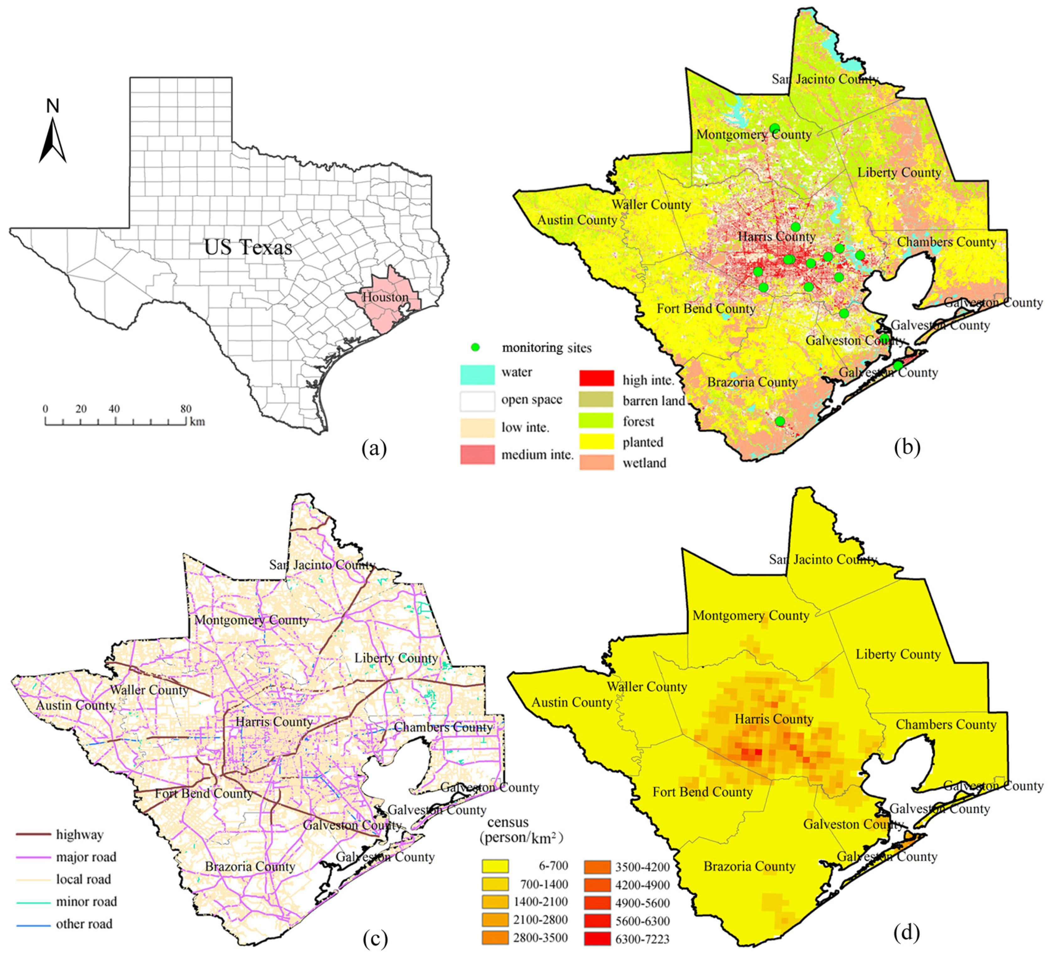
2.1. Study Area and Data Collection
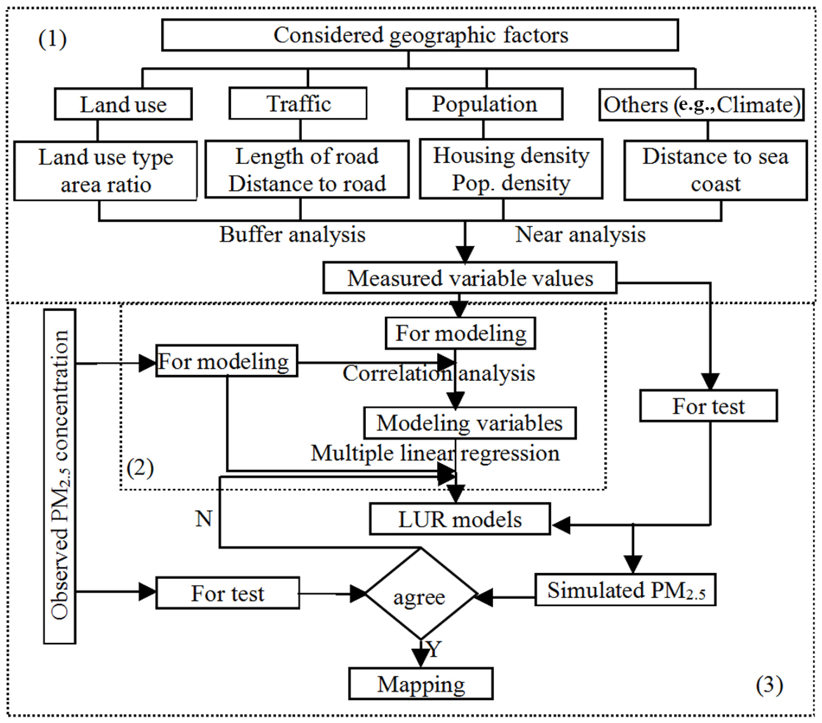
Houston, Texas, USA is a typical urban pollution area with stable geographic and meteorological environment, high air pollution level, and comparatively intensive urban PM2.5 monitoring sites. As the fourth largest metropolitan area in the US, Houston displays significant characteristics that are relevant to urban air pollution. Flat and built on former swampland, the city has a subtropical climate with 1224 mm of precipitation annually and an average temperature of 20.7 °C. It is well known for its petroleum industry, high economic development, and 26% population growth from 2000–2010. In 2011, 17 PM2.5 monitoring sites, which including federal reference monitors (FRM) and federal equivalent method (FEM) monitors which provide measurements on days when FRMs are not recording and at locations without FRMs, were installed across greater Houston. Due to the local industrial production and traffic emission, the annual mean of observed particulate matter concentration ranged from 9.87 μg·m−3 (minimum) to 14.24 μg·m−3 (maximum), and the average value was 11.66 μg·m−3, while, there was only one station within the WHO PM2.5 concentration safety limit (10 μg·m−3) in this region.
Land use (e.g., fraction of built, forest, water, and grass), road traffic, road (e.g., road length, distance to the nearest road), coast (e.g., distance to the nearest coast), population distribution, geographical location, and climate characteristics were considered to be the general factors associated with PM2.5 emission and dispersion in previous LUR research findings [16,23,27,28,32,33,34,35]. Data collected for LUR modeling in this study therefore contains annual average PM2.5 concentration [36], land use/cover in 2011 [37], road network in 2011 [38], and census data in 2010 [39]. The basic geographical data and PM2.5 monitoring sites distribution within the Houston area are shown in Figure 1.

2.2. Study Design

As shown in Figure 2, this study was divided into three parts including extraction of characteristic variables, correlation analysis, and impact analysis of spatial scale on LUR modeling and mapping.

2.2.1. Extraction of Characteristic Variables

As the rules mentioned above, characteristic variables utilized for LUR modeling in this study included area ratio of land use, total road length, distance to nearest road, population density, housing density, and distance to sea coast. All these factors, except distance to nearest road, had obvious spatial scale effects. That is to say, the measured values would vary with the changes of the buffering radius of PM2.5 monitoring sites. The buffering radiuses were set as 100 m, 300 m, 500 m, 800 m, and 1000–5000 m with intervals of 500 m, according to previous research findings [27,28]. For the area ratio (%) of a specific land use type of PM2.5 monitoring site, it was implemented by measuring the area of this land use type and then dividing it by the total area of all land use types within the certain buffering radius of this site. In this process, the original land use types were reclassified into “forest” (Forest11), “open space urban” (O-urban12), “medium intensity urban” (M-urban13), “high intensity urban” (H-urban14), and “barren land” (Barren15) based on the similarity of reducing or increasing PM2.5 concentration diffusion. For characteristic variables of “total road length” (T-length21) and “distance to nearest road” (D-road22), the measured values (unit: km) were computed for the length based on all level roads including highway, major road, local road, minor road, and other road, within certain buffering radius. Similarly, “population density” (P-density31, unit: person/km2) and “housing density” (H-density32, unit: house/km2) were calculated by counting the number of populations and houses, respectively, and then dividing them by the area of each buffering radius. Additionally, spatial scale free variable of “distance to sea coast” (D-coast41, unit: km) was also extracted to indirectly represent the possible influences of other geographical and climate characteristic factors (e.g., wind speed, temperature, and humidity).

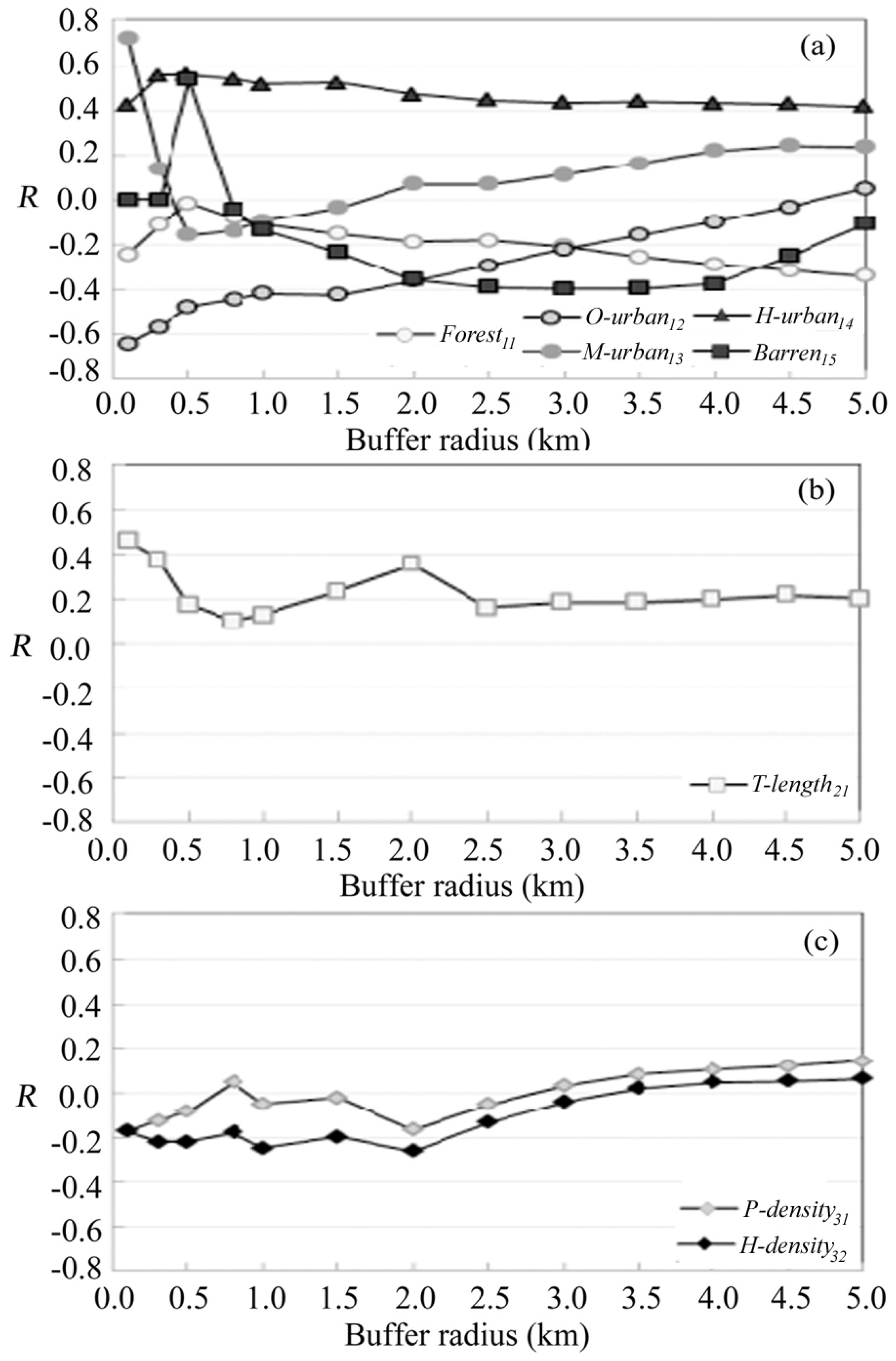
2.2.2. Correlation Analysis

Based on the clear characteristic variables of the model, the aforementioned step for LUR modeling was used to extract the ‘measured values’ of these variables at different preset buffering radiuses. However, these measured values usually varied with the spatial scales, as shown in Table 1, and reported LUR models were plagued on account of a lack of reasonable methods to determine the ideal spatial scales of these measured values [31,40,41]. Therefore, this study attempted to develop a way to initially discern the measured values of characteristic variables at an ideal buffering radius (i.e., optimized spatial scale) to improve the performance of LUR. This procedure was conducted by conducting correlation analyses between all the measured values of characteristic variables at preset various buffering radiuses. The annual mean PM2.5 concentrations were calculated based on the observed measurements from the regulatory monitoring stations. As a result, the measured value of each of the characteristic variables at a relatively ideal buffering radius with regards to the maximum Pearson coefficient could be kept. In contrast, those measured values of variables at irrelevant buffering radiuses would be screened out due to the statistically weaker values of “Pearson coefficient” [42].

2.2.3. Impact Analysis of Spatial Scale on LUR Modeling and Mapping

To validate the feasibility of statistically determining the ideal spatial scale of a characteristic variable in LUR modeling using correlation analysis and its impact on the accuracy of LUR mapping, this study developed all the LUR models both at the ideal buffering radius and relatively irrelevant buffering radiuses. These LUR models were built using SAS analysis (SAS Institute, Cary, NC, USA) and backward multi linear regression (MLR) with non-spatial variables (i.e., distance to sea coast, distance to nearest road). The significant level of t tests less than 0.05 and VIF (Variance Inflation Factors) values less than 5, which were used to control the collinearity between modeling variables, were used as the additional conditions for characteristic variables to determine whether they were introduced into the LUR model or not. Differences of simulation results among LUR models were firstly validated by comparing predicted annual average PM2.5 concentrations with observed concentrations at monitoring sites using the N-1 cross validation strategy. Consequently, in order to demonstrate the outperformance of the LUR model at the optimized spatial scale, annual average PM2.5 concentration surfaces of Houston were produced by LUR models with best, moderate-, and weakest fitting degrees, respectively, as well as ordinary kriging, which is a preferred geostatistical method in air pollution modeling [14]. In this process, a Levene’s test [43] and an F test [44] were also employed to verify the difference between the concentrations extracted from above surfaces with a regular grid size of 3 km × 3 km.

3. Results

3.1. Preliminary Identification of PM2.5 Related Characteristic Variables

Figure 3 demonstrates that the Pearson correlation coefficients between the characteristic variables and annual average PM2.5 concentrations varied with the changes of buffering radiuses (i.e., spatial scales). These correlation coefficients ranged from −0.64 to 0.72 for land use class (Figure 3a), from 0.10 to 0.46 for total road length (Figure 3b), and from −0.26 to 0.14 for population- and housing density (Figure 3c). More importantly, the cross-scale comparison of correlation coefficients identified unique spatial scale effects of different variables. For instance, the area ratios of forest (Forest11) and open space urban (O-urban12) were negatively correlated with annual average PM2.5 concentrations, peaking at 100 m and 5000 m, respectively. The correlations of medium intensity urban (M-urban13), high intensity urban (H-urban14), and barren land (Barren15) with annual average PM2.5 concentrations were most influenced by the scales of 100 m, 500 m, and 3 km. The total road length (T-length21) was positively correlated with annual average PM2.5 concentration, particularly at the 100 m scale, while the correlation coefficients decreased rapidly as the buffering radius increased to 500 m. However, this decreasing trend fluctuated after the buffering radius of 500 m and remained relatively stable at about 0.20. The correlation coefficients of population- (P-density31) and housing density (H-density32) with annual average PM2.5 concentrations varied greatly within 2000 m and decreased thereafter, while the optimized scales for them were 100 m and 2 km, respectively.

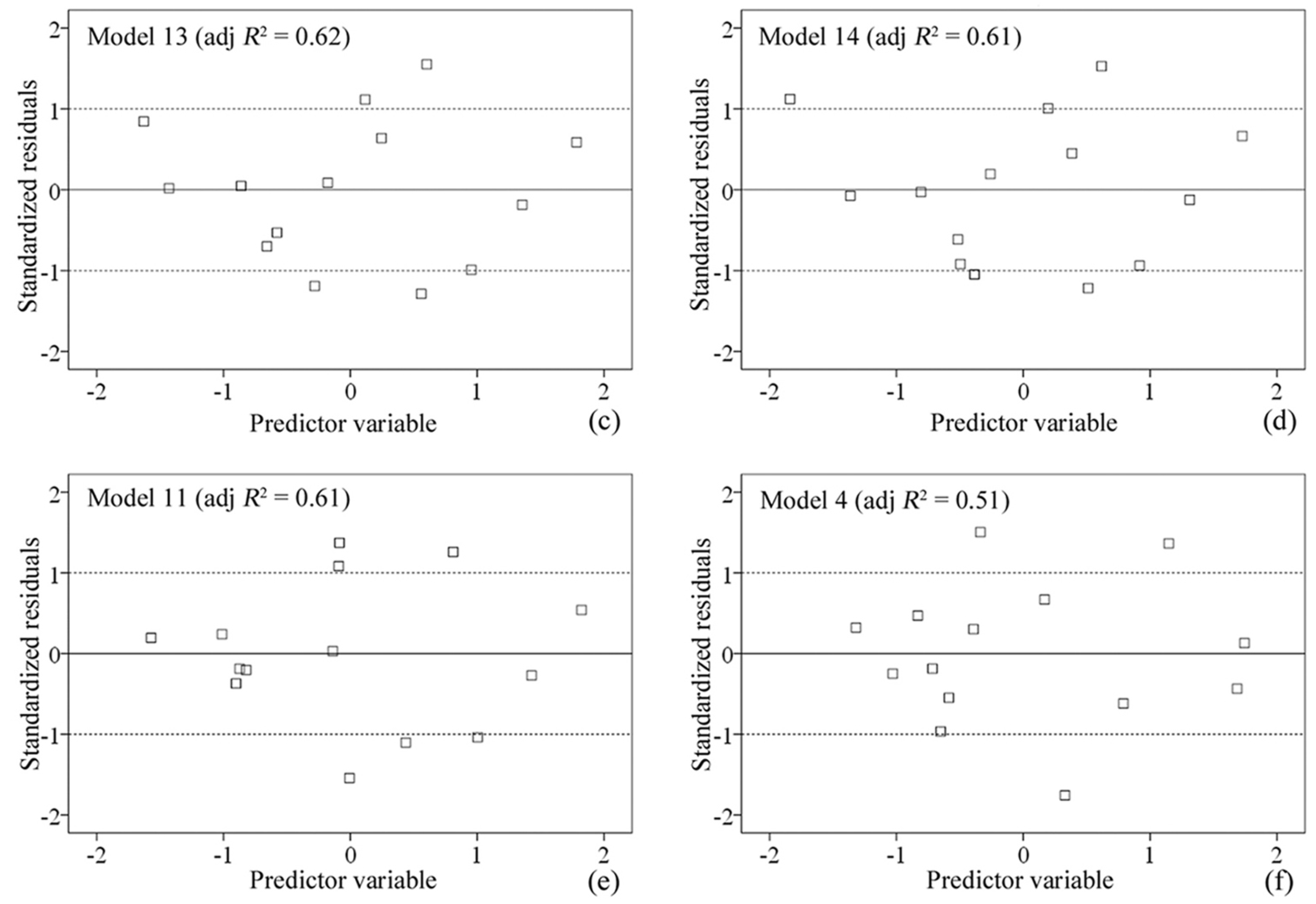
3.2. Performance Validation of LUR Models under Different Spatial Scales

Table 2 illustrates the PM2.5 LUR models built both at ideal buffering radius (optimized spatial scale) and less correlated (non-optimized spatial scale) buffering radiuses, assisted with variables without spatial scale effects but had strong correlations. It can be observed that the LUR model based on variables’ optimized spatial scale measured values obtained the best fitting result (adj. R2 = 0.78). This was followed by models based on variables’ measured values at other less correlated scales of 4 km (adj. R2 = 0.65), 4.5 km (adj. R2 = 0.62), 5 km and 3.5 km (adj. R2 = 0.61), 500 m (adj. R2 = 0.51), and 100 m (adj. R2 = 0.48). Other LUR models had a comparatively lower fitting degree for adjusted R2 ranging from 0.19 to 0.39 at scales from 1 km to 3 km. Moreover, the LUR models in Table 2 also obviously indicated the fluctuations of the predictive variables. Under smaller spatial scales the predictive variables favored medium- (M-urban13) and high intensity urban ratios (H-urban14), total road length (T-length21), as well as distance to nearest road (D-road22). The contributions of housing density (P-density31), high intensity urban ratios (H-density32), and distance to sea coast (D-coast41) increased gradually with the increase in the spatial scales.
To avoid the col-linearity in the MLR process, residual analyses of the six LUR models with relative higher fitting degrees were also conducted in this study. The results in Figure 4 show that all standardized residuals were stochastically distributed, roughly falling at the horizontal zonal area (|r| ≤ 2) without any potential trend. Additionally, the comparison of mean error rate (MER) and root mean squared error (RMSE) for LUR models of PM2.5 simulation concentration in Table 3 further confirmed the reliability of LUR models, with MER under 20%. The model that was established by variables at the optimized spatial scale (Model 1) had the smallest MER of 11.84% and the RMSE value of 1.43.

3.3. PM2.5 Concentration Surfaces Mapped by LUR Models and Ordinary Kriging

As an implementation of LUR modeling, mapping performance is particularly important for correctly understanding the PM2.5 pollution pattern of an area, as illustrated by Figure 5 in this study. Figure 5 shows that there was clearly different annual average PM2.5 concentration surfaces for Houston produced by the LUR models with best- (i.e., Model 1), moderate- (i.e., Model 2), weakest (i.e., Model 7) adjusted R2, as well as ordinary kriging. These differences mean the relative large biases of mapping results of Model 2, Model 7, and ordinary kriging based on the performance validation results of LUR models in Section 3.2. Specifically, for models 1 and 2 the higher annual mean PM2.5 concentrations (i.e., >10 μg·m−3) were distributed in urban Harris County and the surrounding area, except that these high level PM2.5 polluted areas in Model 2 were greater than those in Model 1. However, on the other hand, the results of Model 7 disclosed that almost the entire annual average PM2.5 concentrations in the Houston area were less than 9 μg·m−3, which were inconsistent with the observed PM2.5 concentration values from the regulatory monitoring sites. In addition, results from Levene’s test and F test with p values less than 0.05 in this study echoed these significant differences demonstrated in Figure 5, which indirectly confirms the reliability of the LUR model built at the optimized spatial scale.

4. Discussion

Using LUR-based PM2.5 concentration simulation in Houston, US as a case study, this study explored for the first time the influences of spatial scales of characteristic variables on LUR modeling by employing the idea of statistically optimized analysis. We found that the accuracy of LUR models changed significantly with different spatial scales. The model based on the optimized spatial scale achieved a much higher “fitting degree” (adj. R2 = 0.78) than at any other scales (adj. R2 range from 0.19 to 0.65), which performed better than previous similar study [45]. However, further improvements are needed to broaden the applicability of these research results.

4.1. Results Analysis

Our results demonstrated that land use and road traffic were more related with annual average PM2.5 concentration than population distribution and distance to sea coast. Medium-, high intensity-, and open space urban had the strongest land use correlations; for road traffic, total road length within the 100 m buffer and distance to nearest road were the main correlations. The reason may lie in the fact that PM2.5 in Houston predominately comes from industrial production and transportation emissions [46,47]. Places with greater urbanization and intensive road traffic generally experienced more serious PM2.5 pollution, resulting in the stronger correlations between medium-, high intensity urban and PM2.5 concentrations. However, the impact of population and distance to sea coast was much weaker. PM2.5 from transport emissions diffused slowly and accumulated near roads because of low-lying terrain and building obstructions which increased the correlations between total road lengths, distance to nearest road, and annual average PM2.5 concentrations. This exemplifies why road traffic is the major factor affecting urban PM2.5 pollution worldwide.
Variations of correlation coefficients between the characteristic variables and annual average PM2.5 concentration under different spatial scales identified how the spatial scale setting can significantly influence correlations. At different spatial scales the correlation coefficients changed in both direction and value. Optimized spatial scales differed from different variables, including 5 km for forest, 100 m for open space urban and medium intensity urban, 500 m for high intensity urban, 3 km for barren land, 100 m for total road length, and 2 km for housing density. The variability reflects how diverse geographical factors have different influencing radiuses for PM2.5 pollution. For example, road traffic is an important emission source of PM2.5 and sites closer to road will be exposed to more serious PM2.5 pollution levels that cause a stronger correlation at smaller spatial scales. Similarly, open space urban, medium-, and high intensity urban land use space would have less impact on PM2.5, leading to a smaller influencing radius. However, since only a large amount of forests can significantly reduce PM2.5 pollution dispersion, they may influence PM2.5 pollution at a larger spatial scale (i.e., the optimized spatial scale of forest area ratio in this study was 5 km).
Comparatively, the LUR model in our study based on variables at the optimized spatial scales achieved an impressive R2 (0.78), mean error rate (11.84%), and RMSE (1.43). These results were not only better than those based on variables at other spatial scales in this study (i.e., at the non-optimized spatial scale, the fitting degree ranged between 0.19 and 0.65; maximum mean error rate and RMSE reached to 28.37% and 4.35, respectively), but they also significantly outperform some previous reported adjusted R2 of PM2.5 LUR models for New York, El Paso, and California. The values of adjusted R2 for those studies were 0.64, 0.49, and 0.65, respectively [26,48,49]. In addition, the annual average PM2.5 concentration maps, which were separately produced by the LUR models with the best-, moderate-, weakest adjusted R2, showed that the LUR model with weakest fitting degree could not simulate the distribution of PM2.5 concentrations well, while models with moderate and best fitting degree both showed better simulation results than ordinary kriging with wider concentration scope. This result actually again confirms the significance of the identification of the optimized spatial scale in LUR modeling, which means the PM2.5 distribution disclosed by LUR Model 1 with the best adjusted R2 was more similar with the true scenario.

4.2. Limitations

In Houston, PM2.5 primarily originates from industrial and vehicle emissions, occasional biomass burning, and floating dust. Though this study emphasized several factors (land use, road traffic, population distribution, distance to sea coast, and other geographical features) during LUR modeling and achieved a surrounding annual average PM2.5 concentration simulation, further improvements on the coverage of geographical factors are still required. For example, variables such as real industrial emissions and urban morphologies of microenvironments (e.g., urban ecological landscape index, street canyon, vegetation index, etc.) can be incorporated into PM2.5 LUR modeling [26,50,51]. These variables may provide additional representative descriptions of PM2.5 pollution. Additionally, a recent study shows PM2.5 emissions from unscheduled maintenance, startup, or shutdown activities continue to increase in recent years [52]. LUR models have limited ability to capture such emission events from industries in Houston.
Based on previous research findings, this study took multiple spatial scales of variables into account. While analyses proved the feasibility of deriving an optimized spatial scale in a statistical manner under the currently unclear physical-chemical dispersion mechanism of PM2.5, isometric discrete spatial scales might fail to continuously identify the spatial scale dependence of characteristic variables because it is a relatively crude scheme. Additionally, the spatial scale range from 100 m to 5 km, though it covered the influence radiuses of most variables, may not be able to fully reflect the relationship between some variables with a scope for very small or very large influence (e.g., road traffic, PM2.5 pollution source, distance to chimney, forest, etc.) on PM2.5 pollution [53]. Therefore, future spatial scale dependence analyses could expand or narrow the spatial scale range of the current study and consider differences in variables’ physical and chemical dispersion mechanisms of PM2.5 pollution with more abundant data.
This study applied MLR to establish the PM2.5 LUR model. Although MLR is the most popular LUR regression model with reliable simulation effect [54], it assumes that variables make the same spatial contributions to PM2.5 pollution in any location in the modeling area. However, under real situations, geographical factors have different levels of spatial heterogeneity (except for spatial correlation). Therefore, future LUR model applications can consider adding spatial weights (e.g., establish a geographical weighted model) into existing models to enhance the simulation accuracy of LUR. Meanwhile, the semi-parametric regression model, which takes linear and non-parametric variables into consideration at the same time, might also be a promising way to improve the accuracy of LUR [55].
In addition, the training sample size might be another important factor influencing the accuracy of LUR models. Although the number of monitoring sites used as training samples in the previously reported PM2.5 LUR models ranged from 13 to more than 100 and the surrounding simulation results also had been achieved under few monitoring data [20,53], the results in this study have to be cautiously explained due to the limited monitoring sites employed. Further validation work in regards to considerations surrounding area through the use of many more sampling sites will greatly promote the exploration of the relationship between monitoring sites and the LUR model’s accuracy, which is a critical problem having not been fully considered in LUR modeling field so far.

5. Conclusions

This study represents the first time that a systematic exploration of the influence of spatial scales of characteristic variables on LUR-based PM2.5 concentration estimation modeling was carried out in a statistical manner. It used LUR-based PM2.5 concentration estimation modeling in Houston, US as an example to illustrate how the challenge of the spatial scale clarity can be investigated. Results indicate that statistical based identification of optimized spatial scales of characteristic variables is necessary to ensure the performance of LUR models in mapping PM2.5 distribution without current clearly understood physical-chemical dispersion mechanisms. LUR models at optimized spatial scales were observed to perform better than unified spatial scales. More importantly, this study provides a scientific basis for the spatial scale selection of characteristic variables in future LUR based air pollution mapping.

Acknowledgments

This research work was supported by the National Key Research and Development Program (2016YFC0206205), the National Natural Science Foundation of China (No. 41201384), the Key Laboratory of Geo-informatics of State Bureau of Surveying and Mapping (No. JC201503), the Open Fund of University Innovation Platform, Hunan under Grant 15K132, and the National Geographic Conditions Monitoring of Hunan (HNGQJC201503). Program for the 2016 Young Academic and Technological Leaders of NASG, funded by Key Laboratory of Geo-informatics of NASG. Thanks Guoqing Sun for his contributions in the paper revision.

Author Contributions

Liang Zhai and Bin Zou conceived and designed the experiments; Xin Fang and Yanqing Luo performed the experiments; Liang Zhai, Neng Wan, and Bin Zou analyzed the data; Shuang Li contributed reagents/materials/analysis tools; Bin Zou and Yanqing Luo wrote the paper.

Conflicts of Interest

The authors declare no conflict of interest.

References

  1. Dominici, F.; McDermott, A.; Zeger, S.L.; Samet, J.M. National maps of the effects of particulate matter on mortality: Exploring geographical variation. Environ. Health Perspect. 2003, 111, 39–44. [Google Scholar] [CrossRef] [PubMed]
  2. Dominici, F.; Peng, R.D.; Bell, M.L.; Pham, L.; McDermott, A.; Zeger, S.L.; Samet, J.M. Fine particulate air pollution and hospital admission for cardiovascular and respiratory and respiratory diseases. J. Am. Med. Assoc. 2006, 295, 1127–1134. [Google Scholar] [CrossRef] [PubMed]
  3. Kam, W.; Delfino, R.J.; Schauer, J.J.; Sioutas, C. A comparative assessment of PM2.5 exposures in light-rail, subway, freeway, and surface street environments in Los Angeles and estimated lung cancer risk. Environ. Sci.: Processes Impacts 2013, 15, 234–243. [Google Scholar]
  4. Dergham, M.; Billet, S.; Verdin, A.; Courcot, D.; Cazier, F.; Shirali, P.; Garçon, G. Toxicological impact of air pollution particulate matter (PM2.5) collected under urban, industrial or rural influence: Occurrence of Oxidative stress and inflammatory reaction in BEAS-2B human bronchial epithelial cells (corrected version). Adv. Mater. Res. 2011, 324, 489–492. [Google Scholar] [CrossRef]
  5. NASA (2010) New Map Offers a Global View of Health-Sapping Air Pollution. Available online: http://www.nasa.gov/topics/earth/features/health-sapping.html (accessed on 11 January 2013).
  6. van Donkelaar, A.; Martin, R.V.; Brauer, M.; Kahn, R.; Levy, R.; Verduzco, C.; Villeneuve, P.J. Global estimates of ambient fine particulate matter concentrations from Satellite-based aerosol optical depth: Development and application. Environ. Health Perspect. 2010, 118, 848–855. [Google Scholar] [CrossRef] [PubMed]
  7. The Lancet (2012) Global Burden of Disease Study 2010. Available online: http://www.thelancet.com/themed/global-burden-of-disease (accessed on 26 April 2013).
  8. Liu, S.; Zhang, K. Fine particulate matter components and mortality in Greater Houston: Did the risk reduce from 2000 to 2011? Sci. Total Environ. 2015, 538, 162–168. [Google Scholar] [CrossRef] [PubMed]
  9. Liu, S.; Ganduglia, C.M.; Li, X.; Delclos, G.L.; Franzini, L.; Zhang, K. Short-term Associations of fine particulate matter components and emergency hospital admissions among a privately insured population in greater Houston. Atmos. Environ. 2016, 147, 369–375. [Google Scholar] [CrossRef]
  10. Liu, S.; Ganduglia, C.M.; Li, X.; Delclos, G.L.; Franzini, L.; Zhang, K. Fine particulate matter components and emergency department visits among a privately insured population in greater Houston. Sci. Total Environ. 2016, 566–567, 521–527. [Google Scholar] [CrossRef] [PubMed]
  11. Zou, B.; Pu, Q.; Bilal, M.; Weng, Q.; Zhai, L.; Nichol, J.E. High-resolution satellite mapping of fine particulates based on geographically weighted regression. IEEE Geosci. Remote Sens. Lett. 2016, 13, 495–499. [Google Scholar] [CrossRef]
  12. Fang, X.; Zou, B.; Liu, X.; Troy, S.; Zhai, L. Satellite-based ground PM2.5 estimation using timely structure adaptive modeling. Remote Sens. Environ. 2016, 186, 152–163. [Google Scholar] [CrossRef]
  13. Hoek, G.; Beelen, R.; Hoogh, K.D.; Vienneau, D.; Gulliver, J.; Fischer, P.; Briggs, D. A review of land-use regression models to assess spatial variation of outdoor air pollution. Atmos. Environ. 2008, 42, 7561–7578. [Google Scholar] [CrossRef]
  14. Zou, B.; Wilson, J.G.; Zhan, F.B.; Zeng, Y. Air pollution exposure assessment methods utilized in epidemiological studies. J. Environ. Monit. 2009, 11, 475–490. [Google Scholar] [CrossRef] [PubMed]
  15. Lee, H.J.; Liu, Y.; Coull, B.A.; Schwartz, J.; Koutrakis, P. A novel calibration approach of MODIS AOD data to predict PM2.5 concentrations. Atmos. Chem. Phys. 2011, 11, 7991–8002. [Google Scholar] [CrossRef]
  16. Zou, B.; Luo, Y.; Wan, N.; Zheng, Z.; Sternberg, T.; Liao, Y. Performance comparison of LUR and OK in PM2.5 concentration mapping: A multidimensional perspective. Sci. Rep. 2015, 5. [Google Scholar] [CrossRef] [PubMed]
  17. Zou, B.; Wang, M.; Wan, N.; Wilson, J.G.; Fang, X.; Tang, Y. Spatial modeling of PM2.5 concentrations with a multifactorial radial basis function neural network. Environ. Sci. Pollut. Res. 2015, 22, 10395–10404. [Google Scholar] [CrossRef] [PubMed]
  18. Gilliland, F.; Avol, E.; Kinney, P.; RJerrett, M.; Dvonch, T.; Lurmann, F.; Buckley, T.; Breysse, P.; Keeler, G.; de Villiers, T.; et al. Air pollution exposure assessment for epidemiologic studies of pregnant women and children: Lessons learned from the centers for children’s environmental health and disease prevention research. Environ. Health Perspect. 2005, 113, 1447–1454. [Google Scholar] [CrossRef] [PubMed]
  19. Briggs, D.J.; Collins, S.; Elliot, P.; Fischer, P.; Kingham, S.; Lebret, E.; Pryl, K.; Reeuwijk, H.V.; Smallbone, K.; der Veen, A.V.; et al. Mapping urban air pollution using GIS: A regression-based approach. Int. J. Geogr. Inf. Sci. 1997, 11, 699–718. [Google Scholar] [CrossRef]
  20. Henderson, S.B.; Beckerman, B.; Jerrett, M.; Brauer, M. Application of land use regression to estimate long-term concentrations of traffic-related nitrogen oxides and fine particulate matter. Environ. Sci. Technol. 2007, 41, 2422–2428. [Google Scholar] [CrossRef] [PubMed]
  21. Mavko, M.E.; Tang, B.; George, L.A. A sub-neighborhood scale land use regression model for predicting NO2. Sci. Total Environ. 2008, 2, 68–74. [Google Scholar] [CrossRef] [PubMed]
  22. Chen, L.; Bai, Z.; Su, D.; You, Y.; You, Y.; Li, H.; Quan, L. Application of land use regression to simulate ambient air PM10 and NO2 concentration in Tianjin City. China Environ. Sci. 2009, 29, 685–691. [Google Scholar]
  23. de Hoogh, K.; Wang, M.; Adam, M.; Badaloni, C.; Beelen, R.; Birk, M.; Cesaroni, G.; Cirach, M.; Declercq, C.; Dėdelė, A.; et al. Development of land Use regression models for particle composition in twenty study areas in Europe. Environ. Sci. Technol. 2013, 47, 5778–5786. [Google Scholar] [CrossRef] [PubMed]
  24. Meng, X.; Chen, L.; Cai, J.; Zou, B.; Wu, C.; Fu, Q.; Zhang, Y.; Liu, Y.; Kan, H. A land use regression model for estimating the NO2 concentration in Shanghai, China. Environ. Res. 2015, 137, 308–315. [Google Scholar] [CrossRef] [PubMed]
  25. Hochadel, M.; Heinrich, J.; Gehring, U.; Morgenstern, V.; Kuhlbusch, T.; Link, E.; Wichmann, H.E.; Kramer, U. Predicting long-term average concentrations of traffic-related air pollutants using GIS-based information. Atmos. Environ. 2006, 40, 542–553. [Google Scholar] [CrossRef]
  26. Ross, Z.; Jerrett, M.; Ito, K.; Tempalski, B.; Thurston, G.D. A land use regression for predicting fine particulate matter concentrations in the New York City region. Atmos. Environ. 2007, 41, 2255–2269. [Google Scholar] [CrossRef]
  27. Ho, C.; Chan, C.; Cho, C.; Lin, H.; Lee, J.; Wu, C. Land use regression modeling with vertical distribution measurements for fine particulate matter and elements in an urban area. Atmos. Environ. 2015, 104, 256–263. [Google Scholar] [CrossRef]
  28. Lee, J.; Wu, C.; Hoek, G.; de Hoogh, K.; Beelen, R.; Brunekreef, B.; Chan, C. LUR models for particulate matters in the Taipei metropolis with high densities of roads and strong activities of industry, commerce and construction. Sci. Total Environ. 2015, 514, 178–184. [Google Scholar] [CrossRef] [PubMed]
  29. Wan, N.; Zou, B.; Strenberg, T. A 3-step floating catchment area method for analyzing spatial access to health services. Int. J. Geogr. Inf. Sci. 2012, 26, 1073–1089. [Google Scholar] [CrossRef]
  30. Wan, N.; Zhan, F.B.; Zou, B.; Chow, E. A relative spatial access assessment approach for analyzing potential spatial access to colorectal cancer services in Texas. Appl. Geogr. 2012, 32, 291–299. [Google Scholar] [CrossRef]
  31. Zou, B.; Peng, F.; Wan, N.; Wilson, J.G.; Xiong, Y. Sulfur dioxide exposure and environmental justice: A multi-scale and source-specific perspective. Atmos. Pollut. Res. 2014, 5, 491–499. [Google Scholar] [CrossRef]
  32. Kloog, I.; Koutrakis, P.; Coull, B.A.; Lee, H.J.; Schwartz, J. Assessing temporally and spatially resolved PM2.5 exposures for epidemiological studies using satellite aerosol optical depth measurements. Atmos. Environ. 2011, 45, 6267–6275. [Google Scholar] [CrossRef]
  33. Hystad, P.; Setton, E.; Cervantes, A.; Poplawski, K.; Deschenes, S.; Brauer, M.; van Donkelaar, A.; Lamsal, L.; Martin, R.; Jerrett, M.; et al. Creating national air pollution models for population exposure assessment in Canada. Environ. Health Perspect. 2011, 119, 1123–1129. [Google Scholar] [CrossRef] [PubMed]
  34. Tunno, B.J.; Michanowicz, D.R.; Shmool, J.L.C.; Kinnee, E.; Cambal, L.; Tripathy, S.; Gillooly, S.; Roper, C.; Chubb, L.; Clougherty, J.E. Spatial variation in inversion-focused vs 24-h integrated samples of PM2.5 and black carbon across Pittsburgh, PA. Expo. Sci. Environ. Epidemiol. 2016, 26, 365–376. [Google Scholar] [CrossRef] [PubMed]
  35. Xu, G.; Jiao, L.M.; Zhao, S.L.; Yuan, M.; Li, X.M.; Han, Y.Y.; Zhang, B.; Dong, T. Examining the impacts of land use on air quality from a spatio-temporal perspective in Wuhan, China. Atmosphere 2016, 7, 62. [Google Scholar] [CrossRef]
  36. U.S. EPA (2011). Available online: http://www.epa.gov/airquality/airdata/ad_data_daily.html (accessed on 12 January 2013).
  37. USGS (2011). Available online: http://seamless.usgs.gov (accessed on 13 January 2013).
  38. ESRI. Available online: http://www.openstreetmap.org/#map=5/51.500/-0.100 (accessed on 22 December 2016).
  39. U.S. census bureau (2010). Available online: http://www.census.gov/main/www/access.html (accessed on 10 February 2013).
  40. Mao, L.; Qiu, Y.; Kusano, C.; Xu, X. Predicting regional space-time variation of PM2.5 with land-use regression model and MODIS data. Environ. Sci. Pollut. Res. 2012, 19, 128–138. [Google Scholar] [CrossRef] [PubMed]
  41. Eeftens, M.; Beelen, R.; de Hoogh, K.; Bellander, T.; Cesaroni, G.; Cirach, M.; Declercq, C.; Dėdelė, A.; Dons, E.; de Nazelle, A.; et al. Development of land use regression models for PM2.5, PM2.5 absorbance, PM10 and PMcoarse in 20 European study areas; results of the ESCAPE project. Environ. Sci. Technol. 2012, 46, 11195–11205. [Google Scholar] [CrossRef] [PubMed]
  42. Pearson, K. On lines and planes of closest fit to systems of points is space. Philos. Mag. J. Sci. 1901, 62, 559–572. [Google Scholar] [CrossRef]
  43. Levene, H. Robust tests for equality of variances. In Contributions to Probability and Statistics; Olkin, I., Ed.; Stanford University Press: Palo Alto, CA, USA, 1960; pp. 278–291. [Google Scholar]
  44. Duncan, D.B. Multiple range and multiple F-test. Biometrics 1995, 11, 1–42. [Google Scholar] [CrossRef]
  45. Zhang, K.; Larson, T.; Gassett, A.; Szpiro, A.; Daviglus, M.; Burke, G.; Kaufman, J.; Adar, S. Characterizing spatial patterns of airborne coarse particulate (PM10–2.5) mass and chemical components in three cities: The Multi-Ethnic Study of Atherosclerosis. Environ. Health Perspect. 2014, 122, 823–830. [Google Scholar]
  46. Fraser, M.P.; Yue, Z.; Buzcu, B. Source apportionment of fine particulate matter in Houston, TX, using organic molecular markers. Atmos. Environ. 2003, 37, 2117–2123. [Google Scholar] [CrossRef]
  47. Zou, B.; Zheng, Z.; Wan, N.; Qiu, Y.H.; Wilson, J.G. An optimized spatial proximity model for fine particulate matter air pollution exposure assessment in areas of sparse monitoring. Int. J. Geogr. Inf. Sci. 2016, 30, 1–21. [Google Scholar] [CrossRef]
  48. Olvera, H.A.; Garcia, M.; Li, W.; Yang, H.; Amaya, M.A.; Myers, O.; Burchiel, S.W.; Berwick, M.; Pingitore, N.E., Jr. Principal component analysis optimization of a PM2.5 land use regression model with small monitoring network. Sci. Total Environ. 2012, 425, 27–34. [Google Scholar] [CrossRef] [PubMed]
  49. Beckerman, B.S.; Jerrett, M.; Martin, R.V.; van Donkelaar, A.; Ross, Z.; Burnett, R.T. Application of the deletion/substitution/addition algorithm to selecting land use regression models for interpolating air pollution measurements in California. Atmos. Environ. 2013, 77, 172–177. [Google Scholar] [CrossRef]
  50. Yu, H.; Wang, C.; Liu, M.; Kuo, Y. Estimation of fine particulate matter in Taipei using land use regression and bayesian maximum entropy methods. Int. J. Environ. Res. Public Health 2011, 8, 2153–2169. [Google Scholar] [CrossRef] [PubMed]
  51. Xu, S.; Zou, B.; Pu, Q.; Guo, Y. Impact Analysis of Land Use/Cover on Air Pollution. J. Geogr. Sci. 2015, 3, 287–297. (In Chinese) [Google Scholar]
  52. Luong, C.; Zhang, K. An Assessment of Emissions Events Trends within the Greater Houston Area during 2003-2013. Air Qual., Atmos. Health 2016. [Google Scholar] [CrossRef]
  53. Chen, C.; Wu, C.; Yu, H.; Chan, C.; Cheng, T. Spatiotemporal modeling with temporal-invariant variogram subgroups to estimate fine particulate matter PM2.5 concentrations. Atmos. Environ. 2012, 54, 1–8. [Google Scholar] [CrossRef]
  54. Ryan, P.H.; LeMasters, G.K. A review of land-use regression models for characterizing intra-urban air pollution exposure. Inhalation Toxicol. 2007, 19, 127–133. [Google Scholar] [CrossRef] [PubMed]
  55. Szyszkowicz, M.; Mahmud, M.; Tremblay, N. A semi-parametric regression model to estimate variability of NO2. Environ. Pollut. 2013, 2, 46–50. [Google Scholar] [CrossRef]
Figure 1. Study area and PM2.5 monitoring site: (a) Study area; (b) PM2.5 monitoring site and land use/cover; (c) road network; (d) census data.
Atmosphere 08 00001 g001
Figure 2. Framework of study procedure. LUR, land use regression. (1) Variables extraction; (2) Variables screen; (3) LUR model fitting and cross-validation.
Atmosphere 08 00001 g002
Figure 3. Correlation coefficients between characteristic variables and annual average PM2.5 concentrations: (a) land use; (b) road traffic; (c) population and housing density.
Atmosphere 08 00001 g003
Figure 4. Standardized residual error map of LUR models: (a) Model 1; (b) Model 12; (c) Model 13; (d) Model 14; (e) Model 11; (f) Model 4.
Atmosphere 08 00001 g004aAtmosphere 08 00001 g004b
Figure 5. PM2.5 concentration surfaces of Houston based on LUR models and ordinary kriging.
Atmosphere 08 00001 g005
Table 1. Statistics of “measured values” (mean (min, max), Units: as listed in Section 2.1).
VariablesMeasured ValuesVariablesMeasured ValuesVariablesMeasured ValuesVariablesMeasured Values
Forest11-500031.95 (0.16, 73.18)M-urban13-500021.07 (5.37, 45.72)Barren15-50000.64 (0.00, 3.48)P-density31-5000574.35 (155.31, 1719.81)
Forest11-450030.25 (0.09, 70.08)M-urban13-450022.09 (5.36, 46.08)Barren15-45000.49 (0.00, 2.19)P-density31-4500568.81 (159.48, 1691.27)
Forest11-400028.41 (0.10, 66.52)M-urban13-400022.48 (5.59, 44.89)Barren15-40000.40 (0.00, 2.25)P-density31-4000543.95 (163.63, 1609.78)
Forest11-350026.30 (0.05, 63.76)M-urban13-350022.47 (5.58, 42.55)Barren15-35000.37 (0.00, 2.54)P-density31-3500554.16 (143.52, 1700.21)
Forest11-300023.86 (0.05, 62.41)M-urban13-300022.71 (5.69, 39.13)Barren15-30000.33 (0.00, 2.34)P-density31-3000706.87 (128.20, 2536.17)
Forest11-250021.46 (0.05, 56.23)M-urban13-250022.93 (7.63, 41.70)Barren15-25000.36 (0.00, 2.22)P-density31-2500552.94 (108.41, 1859.69)
Forest11-200017.98 (0.00, 44.52)M-urban13-200023.65 (10.23, 43.70)Barren15-20000.36 (0.00, 2.07)P-density31-2000686.97 (85.69, 2558.86)
Forest11-150012.96 (0.00, 35.46)M-urban13-150024.25 (10.1, 42.78)Barren15-15000.41 (0.00, 2.70)P-density31-1500609.19 (83.05, 1744.41)
Forest11-10009.95 (0.00, 30.46)M-urban13-100024.57 (7.87, 44.43)Barren15-10000.31 (0.00, 3.26)P-density31-1000687.06 (94.90, 1652.37)
Forest11-8008.36 (0.00, 26.11)M-urban13-80025.56 (7.23, 47.13)Barren15-8000.24 (0.00, 2.39)P-density31-800635.68 (77.56, 1958.88)
Forest11-5005.80 (0.00, 18.82)M-urban13-50025.17 (10.78, 50.59)Barren15-5000.02 (0.00, 0.31)P-density31-500589.57 (24.73, 1359.31)
Forest11-3003.48 (0.00, 19.32)M-urban13-30023.55 (9.13, 41.76)Barren15-3000.00 (0.00, 0.00)P-density31-300555.93 (24.87, 1400.62)
Forest11-1000.75 (0.00, 10.45)M-urban13-10021.79 (0.00, 48.78)Barren15-1000.00 (0.00, 0.00)P-density31-100509.19 (24.67, 1389.24)
O-urban12-500032.22 (11.06, 55.30)H-urban14-500013.49 (3.05, 36.42)T-length21-5000458.93 (202.46, 1104.14)H-density32-5000201.90 (57.11, 669.74)
O-urban12-450033.04 (12.87, 55.22)H-urban14-450014.12 (2.92, 38.63)T-length21-4500390.49 (174.75, 977.80)H-density32-4500197.99 (56.30, 640.30)
O-urban12-400033.79 (12.48, 54.16)H-urban14-400014.91 (2.51, 41.99)T-length21-4000306.33 (123.91, 765.44)H-density32-4000187.03 (48.61, 592.81)
O-urban12-350034.78 (10.95, 52.14)H-urban14-350016.07 (2.36, 45.92)T-length21-3500238.98 (80.52, 605.11)H-density32-3500188.16 (40.68, 618.35)
O-urban12-300036.45 (10.60, 56.73)H-urban14-300016.65 (2.34, 49.67)T-length21-3000188.69 (53.10, 489.08)H-density32-3000240.04 (37.25, 913.73)
O-urban12-250038.16 (10.45, 64.74)H-urban14-250017.09 (3.01, 55.39)T-length21-2500131.09 (30.94, 328.16)H-density32-2500181.78 (33.11, 645.51)
O-urban12-200040.16 (10.92, 71.96)H-urban14-200017.85 (3.25, 59.95)T-length21-200088.05 (23.51, 214.96)H-density32-2000225.16 (28.27, 872.09)
O-urban12-150043.62 (11.07, 75.23)H-urban14-150018.77 (3.25, 68.21)T-length21-150052.19 (18.15, 128.37)H-density32-1500183.94 (27.67, 565.37)
O-urban12-100046.22 (6.75, 79.01)H-urban14-100018.95 (2.92, 77.30)T-length21-100023.27 (9.53, 60.66)H-density32-1000211.81 (31.75, 560.28)
O-urban12-80047.20 (6.50, 77.84)H-urban14-80018.64 (1.83, 79.98)T-length21-80014.90 (5.76, 39.44)H-density32-800183.35 (24.03, 448.72)
O-urban12-50051.72 (6.49, 77.28)H-urban14-50017.29 (1.09, 76.29)T-length21-5005.65 (1.46, 15.22)H-density32-500186.44 (7.97, 450.35)
O-urban12-30056.43 (8.44, 88.25)H-urban14-30016.55 (2.62, 72.68)T-length21-3001.98 (0.22, 5.67)H-density32-300176.91 (8.02, 460.55)
O-urban12-10062.56 (0.00, 100.00)H-urban14-10014.90 (0.00, 69.78)T-length21-1000.21 (0.00, 0.68)H-density32-100169.69 (7.95, 456.81)
D-road2279.67 (0.18, 279.51)D-coast4155.39 (1.38, 125.15)
Table 2. Predictors and adjusted R2 of LUR models for PM2.5 concentration simulation.
Model IDSpatial ScaleModel PredictorsModel R2
1Best scaleM-urban13-100, P-density31-100, Forest11-50000.78
2100 mM-urban13-1000.48
3300 mT-length21-300, H-urban14-300, D-road220.45
4500 mT-lenegth21-500, H-urban14-500, D-road220.51
5800 mT-length21-800, H-urban14-8000.39
61000 mH-urban14-10000.21
71500 mD-coast41, O-urban12-1500, P-density31-15000.19
82000 mH-density32-2000, O-urban12-2000, Forest11-20000.30
92500 mH-density32-2500, H-urban14-25000.38
103000 mH-density32-3000, H-urban14-30000.34
113500 mH-density32-3500, D-coast41, H-urban14-35000.61
124000 mH-density32-4000, D-coast41, H-urban14-40000.65
134500 mH-density32-4500, D-coast41, H-urban14-45000.62
145000 mH-density32-5000, D-coast41, H-urban14-50000.61
Table 3. Comparison of mean error rate (MER) and root mean squared error (RMSE) for LUR models of PM2.5 concentration simulation.
Model IDMER (%) 1RMSE (μg·m−3)
111.841.43
217.222.65
316.732.45
416.781.97
519.933.13
628.264.16
728.374.35
827.323.87
919.303.26
1026.323.69
1114.371.72
1215.031.80
1315.581.87
1413.211.58
1 MER = |Observed concentration − Simulated concentration|/Observed concentration × 100%.

