Article

Intercomparison of Carbon Dioxide Products Retrieved from GOSAT Short-Wavelength Infrared Spectra for Three Years (2010–2012)

1
Institute of Remote Sensing and Digital Earth, Chinese Academy of Sciences, 20A North Datun Road, Beijing 100101, China
2
School of Surveying and Land Information Engineering, Henan Polytechnic University, 2001 Century Road, Jiaozuo 454000, China
3
University of Chinese Academy of Sciences, 19A Yuquan Road, Beijing 100049, China
*
Author to whom correspondence should be addressed.
Atmosphere 2016, 7(9), 109; https://doi.org/10.3390/atmos7090109
Submission received: 28 July 2016 / Revised: 17 August 2016 / Accepted: 18 August 2016 / Published: 23 August 2016

Abstract

:
This paper presents the comparison of two CO2 datasets from the National Institute for Environmental Studies (NIES) of Japan and the Atmospheric CO2 Observations from Space (ACOS) of NASA for three years (2010 to 2012). Both CO2 datasets are retrieved from the Greenhouse gases Observing SATellite (GOSAT) short-wavelength infrared spectra over High gain surface land. In this three-year period, the yield of the NIES CO2 column averaged dry air mole fractions (XCO2) is about 71% of ACOS retrievals. The overall bias is 0.21 ± 1.85 ppm and −0.69 ± 2.13 ppm for ACOS and NIES XCO2, respectively, when compared with ground-based Fourier Transform Spectrometer (FTS) observations from twelve Total Carbon Column Observing Network (TCCON) sites. The differences in XCO2 three-year means and seasonal means are within about 1 to 2 ppm. Strong consistency is obtained for the ACOS and NIES XCO2 monthly averages time series over different regions, with the greatest mean difference of ACOS to NIES monthly means over China (1.43 ± 0.60 ppm) and the least over Brazil (−0.03 ± 0.64 ppm). The intercomparison between the two XCO2 datasets indicates that the ACOS XCO2 is globally higher than NIES by about 1 ppm and has smaller bias and better consistency than NIES data.

1. Introduction

Atmospheric carbon dioxide (CO2) is the most important greenhouse gas. The column averaged dry air mole fractions of atmospheric CO2 (XCO2) has increased dramatically from 280 parts per million (ppm) in the pre-industrial era to 396 ppm in 2013 [1], most probably due to human activities, such as fossil fuel combusting, land use change, cement production and biomass burning. The resulting warming effect of increasing CO2 concentration is predicted to lead to a rising surface temperature, rising sea levels and frequent occurrence of extreme weather conditions [2]. To reliably predict the impact of atmospheric CO2 on global climate change, it is necessary to clarify the distribution and variation of atmospheric CO2 concentration, as well as its source and sink.
Ground-based observations of greenhouse gas can provide accurate and high–frequent CO2 measurements. However, their sparse and uneven global distributions lead to large uncertainties in the estimates of CO2 amount and flux on sub-continental or regional spatial scales [3,4,5]. Theoretical studies show that satellite retrieval of atmospheric CO2 has the potential to significantly reduce the uncertainties in estimated CO2 surface flux if the satellite observations are accurate and precise enough [6,7,8,9].
Greenhouse gases Observing SATellite (GOSAT) [10], launched in January 2009, was the world’s first dedicated carbon satellite and has provided global multi-year observations with significant sensitivity near the surface. Based on the Short-Wavelength InfraRed (SWIR) spectra of GOSAT, two XCO2 products were retrieved independently: the XCO2 official product from the National Institute for Environmental Studies (NIES) of Japan [11,12,13] and the XCO2 data product from Atmospheric CO2 Observations from Space (ACOS) of NASA [14,15,16]. The research on the two products was extensive. Morino et al. [12] validated NIES GOSAT SWIR Level 2 v01.xx XCO2 against the ground-based Fourier Transform Spectrometer (FTS) XCO2 observations from the Total Carbon Column Observing Network (TCCON) and found that the NIES XCO2 was biased by −8.85 ± 4.75 ppm. Yoshida et al. [13] presented that the NIES Level 2 v02.xx XCO2 from an improved retrieval algorithm showed much smaller bias and standard deviation (−1.48 and 2.09 ppm). Inoue et al. [17] compared NIES Level 2 v02.xx XCO2 with aircraft-based data and the NIES XCO2 was biased by −0.68 ± 2.56 ppm. Lei et al. [18] showed the comparison of NIES Level 2 v02.xx XCO2 with model simulations and found that the XCO2 was globally lower than the model by 2 ppm on average. For ACOS XCO2, Crisp et al. [16] reported the estimates of XCO2 and analyzed the XCO2 retrieval error characteristics. The preliminary validation of ACOS Level 2 v3.3 XCO2 against TCCON data showed that the mean bias and standard deviation were 1.34 and 1.83 ppm [19]. Zhang et al. [20] examined the difference between ACOS Level 2 v3.3 XCO2 and model simulations and found that the retrieved XCO2 was higher than model by 0.11 ± 1.81 ppm. Lindqvist et al. [21] evaluated the ACOS v3.5 XCO2 seasonal cycle features with TCCON data. Kulawik et al. [22] validated the precision characteristics, season cycle, yearly growth and daily variability of ACOS v3.5 XCO2 based on TCCON data.
These XCO2 products were validated or compared with ground-based FTS data or model simulations. However, the validations or comparisons of the two XCO2 products were carried out individually. The different characteristics between them remain unknown for different regions and times. Therefore, detailed analyses of the differences and suitabilities between the two XCO2 products are essential for the evaluation of CO2 retrieval algorithms and the combined applications of the two products, for example, combining the two products to generate improved datasets, and, in turn, to improve model prediction of global CO2 source/sink. In this paper, we compare the NIES GOSAT SWIR Level 2 v02.xx XCO2 (NIES XCO2) and ACOS GOSAT Level 2 v3.5 XCO2 (ACOS XCO2) over land surfaces with High gain for the period of 2010 to 2012. We examine the difference of these two XCO2 datasets to provide references for the evaluation of CO2 retrieval algorithms and the suitability of the XCO2 products in applications.
The paper is structured as follows. In Section 2, we describe the GOSAT and instruments, NIES and ACOS GOSAT XCO2 products, and the main differences in ACOS and NIES XCO2 retrieval algorithms. Section 3 presents the intercomparison and analysis between NIES and ACOS XCO2 datasets for three years, and Section 4 provides the conclusions.

2. Data and Method

The analyzed time period spans three years, ranging from January 2010 to December 2012. The NIES GOSAT SWIR Level 2 v02.xx XCO2 product and ACOS GOSAT Level 2 v3.5 XCO2 retrievals are collected for the entire study period. As differences in the retrieval results still remain because of the High/Medium gain and land/ocean differences, the comparisons between NIES and ACOS XCO2 are limited to High gain land surface in this work.

2.1. GOSAT and Instruments

GOSAT, which was launched on 23 January 2009, was the world’s first satellite dedicated to measure the atmospheric CO2 and methane (CH4). GOSAT was put in a sun-synchronous orbit at about 666 km with three-day recurrence. It was equipped with two instruments: Thermal and Near infrared Sensor for carbon Observation-Fourier Transform Spectrometer (TANSO-FTS) and Cloud and Aerosol Imager (TANSO-CAI). TANSO-FTS is a Michelson interferometer and observes high-resolution spectra in three SWIR bands: 12,900 to 13,200 cm−1 with 0.37 cm−1 spectral resolution, 5800 to 6400 cm−1 and 4800 to 5200 cm−1 with 0.26 cm−1 spectral resolution, and a TIR band: 700 to 1800 cm−1 with 0.26 cm−1 spectral resolution. The instantaneous field view of TANSO-FTS is about 15.8 mrad, corresponding to a nadir footprint diameter of about 10.5 km at sea level. The high spectral resolution spectra recorded by TANSO-FTS are analyzed to produce CO2 and CH4 products. TANSO-CAI is a radiometer used to detect optically thick clouds and aerosol inside the TANSO-FTS’s field of view. For details on the GOSAT and the instruments, please refer to Kuze et al. [23].

2.2. NIES and ACOS GOSAT XCO2 Products

The NIES GOSAT XCO2 data analyzed in this paper are the TANSO-FTS SWIR Level 2 v02.xx XCO2 product, which was produced by NIES of Japan. The NIES XCO2 product was retrieved from the absorption spectra within the three SWIR bands and represent XCO2 of a single measure point. All the column abundances of CO2 were successfully retrieved and passed the post-screening criteria [11,12,13]. After an improvement of the retrieval algorithm from v01.xx to 02.xx, the accuracy and precision of NIES GOSAT SWIR XCO2 has been improved significantly. The bias and standard deviation of NIES GOSAT v02.xx XCO2 were estimated to be about −1.48 ppm and 2.09 ppm against the ground-based FTS XCO2 data from the TCCON sites [12,13].
After the loss of the Orbiting Carbon Observatory (OCO), the OCO science team was reformulated as the ACOS team by NASA and was invited to analyze the GOSAT data [15,16]. The ACOS GOSAT XCO2 used here was the Level 2 v3.5 XCO2 retrieved from GOSAT TANSO-FTS SWIR Level 1B data. The ACOS XCO2 standard product contained all the soundings that converged in the retrieval [16,24]. According to the recommendations of ACOS Level 2 Standard Product Data User’s Guide v3.5, the data screening and bias correction were applied to ACOS XCO2 before use [24].

2.3. The Main Differences between ACOS and NIES GOSAT XCO2 Retrieval Algorithms

Although both ACOS and NIES GOSAT SWIR L2 XCO2 retrieval algorithms are based on the optimal estimation methods [11,13,15,16,25,26,27], there are still some specific differences between them. The NIES v02.xx retrieval algorithm conducts strict cloud screening and simultaneously retrieves the vertical profile of four typical aerosol species [13]. While there was no similar sensor sensitive to clouds on OCO-2, the ACOS L2 v3.5 retrieval algorithm applied Oxygen-A band only clear-sky retrieval to screen optically thick clouds, and retrieved the profile of two aerosol types and two cloud types simultaneously [15,24]. These differences in the handling of light scattering may lead to different retrieval results. The CO2 absorption cross-sections around 2.06 um band were scaled by 0.99 to get more consistent results with the 1.61 um band in the ACOS retrieval algorithm [19]. This could cause large changes in the XCO2 retrieval results. There were still some differences in the pre-/post-processing between the two retrieval algorithms, such as the solar zenith angles requirements, and the aerosol optical depth (AOD) filtering [13,15,16,24]. These factors could affect the yields of the retrieval algorithm. In addition, to get high quality retrieval results, the ACOS XCO2 are screened using the updated screening criteria and underwent the bias correction to correct global bias and errors additionally according to the recommendations of ACOS [14,16,24]. This could further improve the consistency of the ACOS retrieval with respect to TCCON observations.

3. Results and Discussion

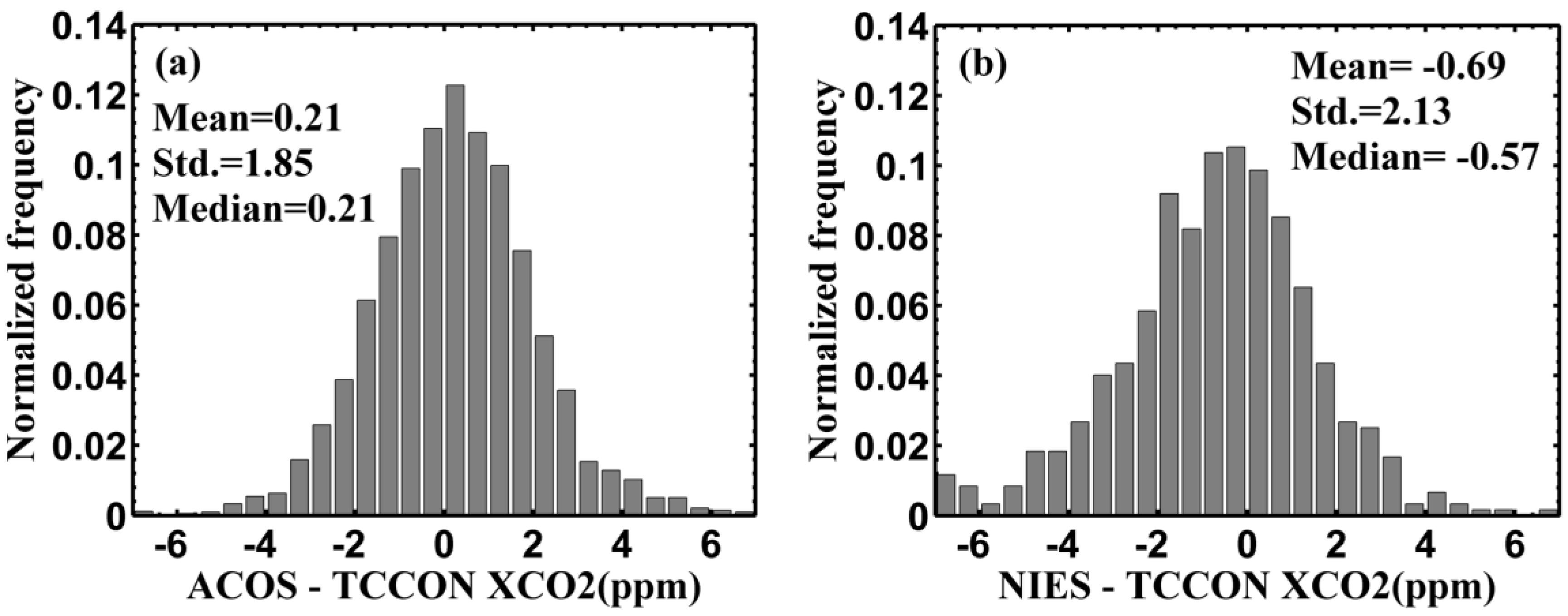
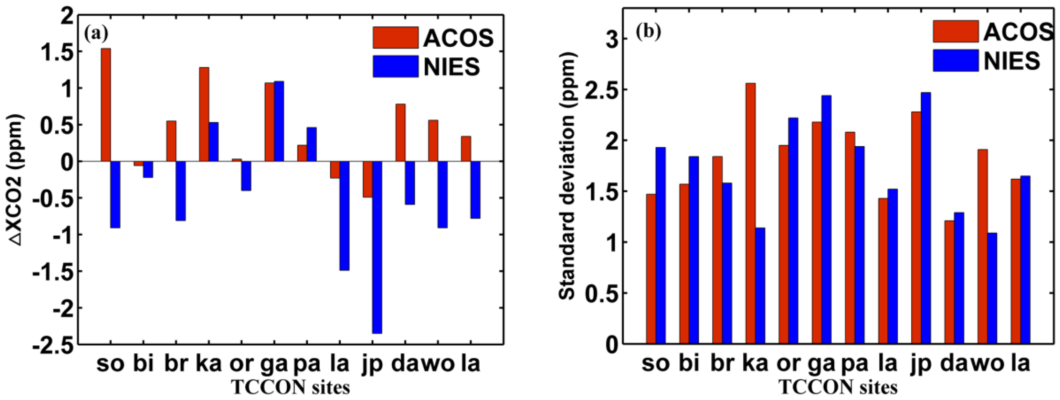
3.1. Comparisons with TCCON XCO2

In order to quantitatively examine the differences between the ACOS and NIES XCO2, the ACOS and NIES XCO2 datasets are compared with ground-based FTS XCO2 observations from twelve TCCON sites shown in Table 1. The ground-based FTS records high spectral resolution (0.02 cm1) direct solar spectra in the near infrared spectrum and the CO2 column concentrations are determined using the GGG software (GGG 2014, California Institute of Technology, California, CA, USA) based on the nonlinear least squares fitting. The uncertainty of the TCCON XCO2 is estimated to be about 0.2% [28,29]. The TCCON data used here are the GGG2014 releases. To get matched data between satellite retrieval and ground-based data, the ground-based FTS data are within ±30 min of GOSAT overpass time and averaged. The satellite retrievals data are collected within a ±3 degrees latitude/longitude box centered at each FTS site. The comparison results are listed in Table 1, and the bias and corresponding standard deviation of each site are shown in Figure 1.
According to Table 1, both ACOS and NIES XCO2 are in good agreement with ground-based data from the correlation coefficients, with the mean correlation coefficients of ACOS and NIES with respect to TCCON 0.76 and 0.73, respectively. The station biases of ACOS XCO2 show most positive values with the exception of Bialystok, Lamont and JPL Pasadena, while the NIES XCO2 shows the mostly negative bias with the exception of Karlsruhe, Garmisch and Park Falls sites. In addition, according to Figure 1, the standard deviation of ACOS is slightly larger than that of NIES for most sites.
Figure 2 shows the histograms of differences of ACOS relative to TCCON and NIES relative to TCCON for all TCCON sites. The overall bias for ACOS and NIES are 0.21 and −0.69 ppm, respectively. The standard deviation of XCO2 differences for ACOS (1.85 ppm) is slightly smaller than NIES (2.13 ppm), indicating better consistency and less potential outliers. The relative accuracy, which indicates the relative regional-scale accuracy, is another important error estimate. The relative accuracy is 0.62 ppm for ACOS and 0.93 ppm for NIES dataset, as reported in Table 1. Through comparison with TCCON XCO2, the ACOS dataset is globally higher than NIES by about 1 ppm on average. In addition, the ACOS has smaller bias and standard deviation than NIES. Since the ACOS retrievals underwent recommended bias correction where the bias-correcting variables and coefficients were derived from TCCON and model data [14,16,24], the agreement between ACOS and TCCON data was improved substantially.

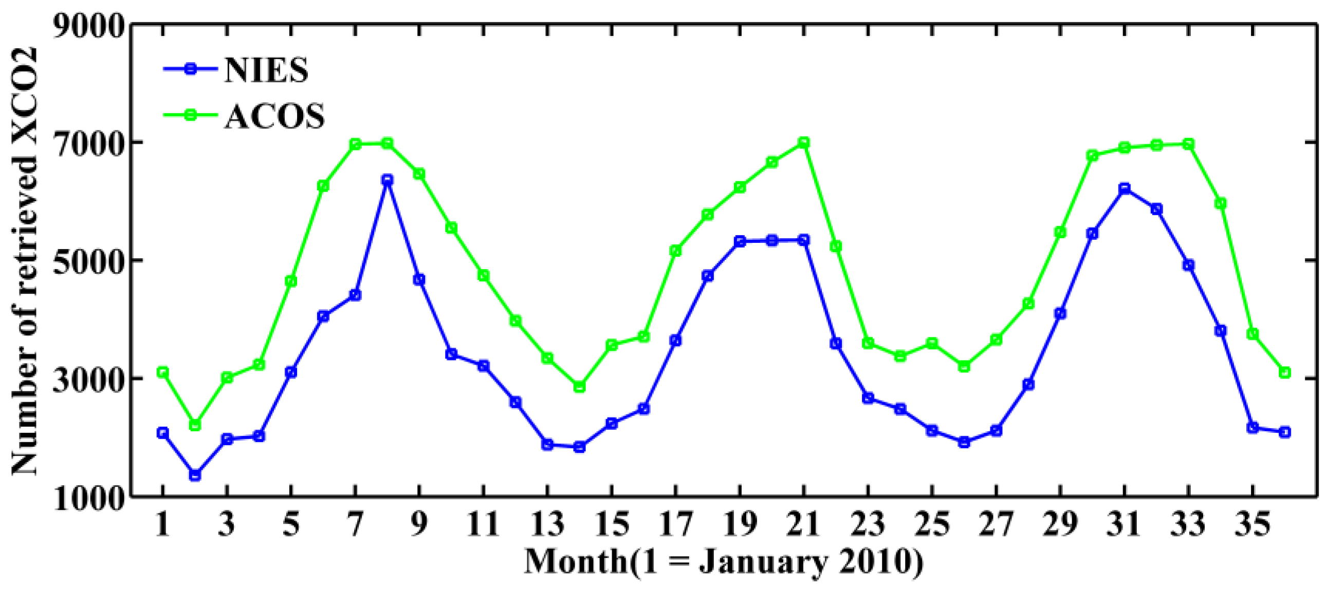
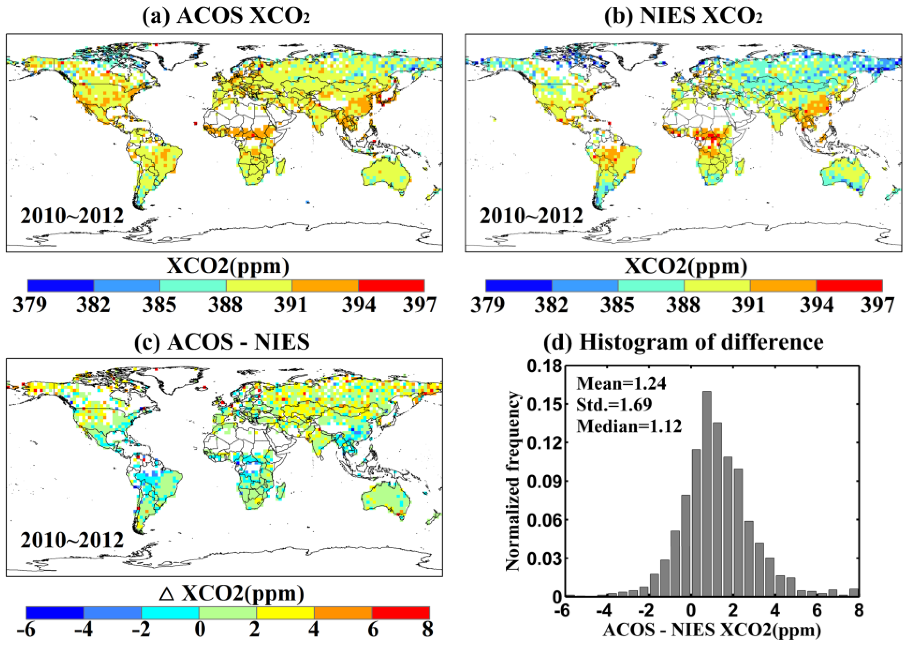
3.2. Comparisons of XCO2 Yields and Three-Year Averages

As seen in Table 1, the number of ACOS retrievals matched with TCCON data is significantly more than NIES. In order to compare the yields of ACOS and NIES XCO2 retrievals, Figure 3 presents the monthly numbers of global ACOS and NIES dataset over High gain land surface. Both ACOS and NIES XCO2 datasets plotted in Figure 3 passed the post-screening filters. According to Figure 3, the yield of NIES XCO2 is averagely 71% of that of ACOS retrievals, with the monthly number rates of NIES to ACOS ranging from 56% to 91%. Multiple factors contribute to the different yields. The NIES retrievals are limited to satellite scenes with solar zenith angles less than 70 degrees, which is less than that of ACOS (85 degrees) [11,16] and eliminates more NIES soundings in the pre-processing. The strategy and methods for cloud screening in ACOS retrievals differ from NIES and could also lead to different yields [11,13,16]. The more rigorous aerosol optical depth (AOD) filter in the NIES post-screening also rejects more retrievals than ACOS [13,16,24]. The number of XCO2 retrievals showing a large seasonal variation also can be seen in Figure 3. This is because the GOSAT soundings with large solar zenith angles in northern high latitudinal regions in winter and early spring are filtered out. The snow-/ice-covered measurements are also removed by the blended albedo filter [13]. Furthermore, the content of desert dust and Asia aerosol is larger in Northern Hemisphere winter and spring and the GOSAT retrievals with high AOD are filtered out [13]. This seasonal characteristic of the desert dust and Asia aerosol could also contribute to the seasonal variations.
Figure 4 shows the three-year average of ACOS and NIES XCO2 and their differences (ACOS–NIES) from 2010 to 2012. The XCO2 means are averaged only when there are more than three XCO2 retrievals in each 2.5° × 2.5° latitude/longitude bin. As can be seen, the distribution of XCO2 three-year averages of ACOS and NIES are very similar, with the correlation coefficient between the three-year averages of ACOS and NIES r = 0.73. The highest values are mainly located in East Asia, Central Africa, Northeast North American, and Central South America from both ACOS and NIES averages, indicating intense human activity and large carbon emissions over these regions. Moreover, about 80.3% of ACOS XCO2 means are greater than NIES data as reported in Figure 4c. The mean difference between ACOS and NIES means is about 1.24 ppm with the standard deviation of 1.69 ppm as reported in Figure 4d.

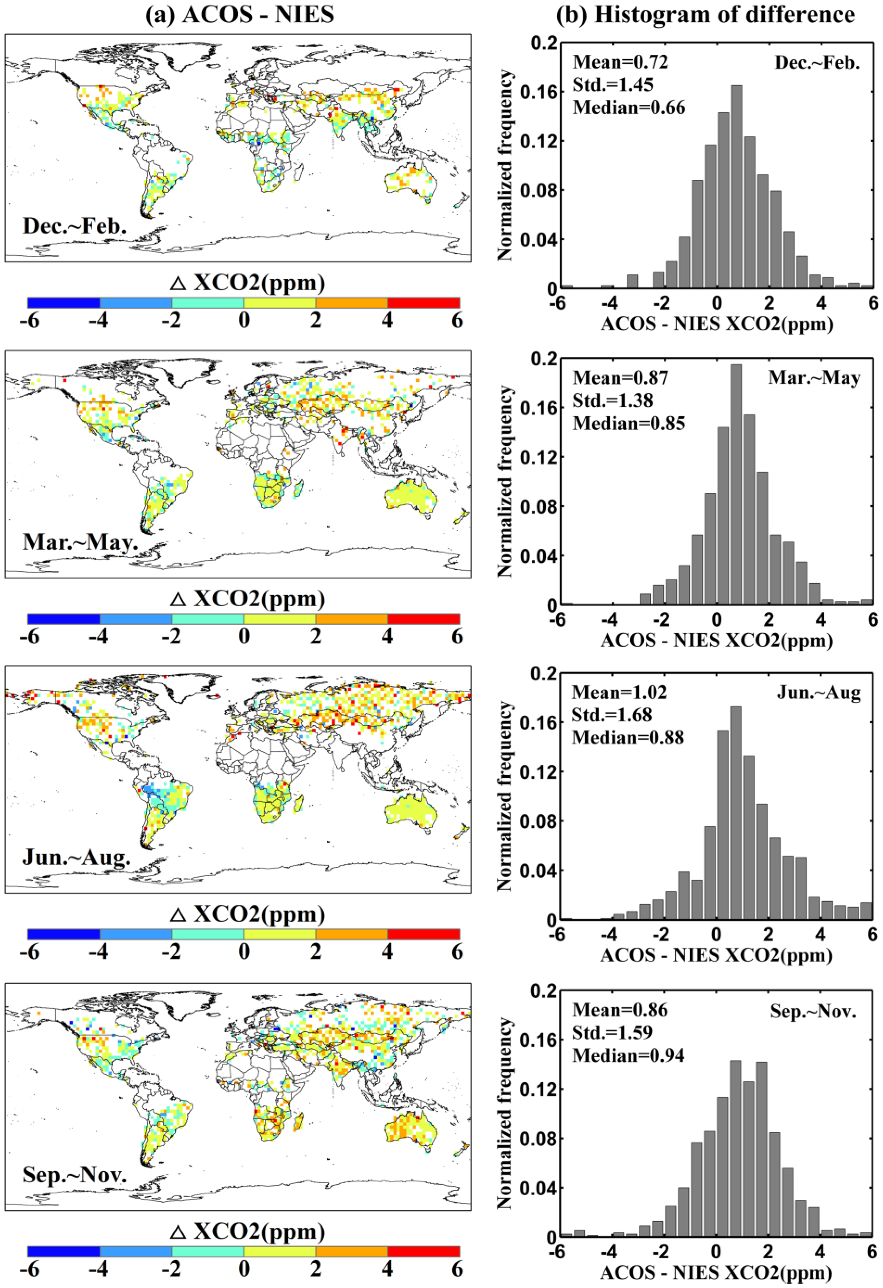
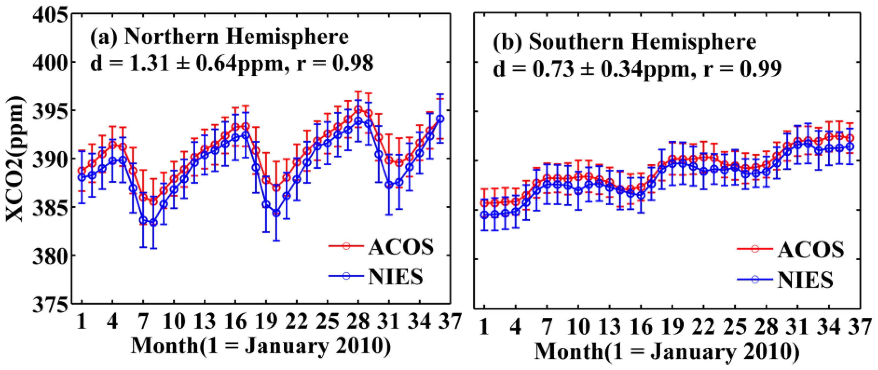
3.3. Seasonal Difference between ACOS and NIES XCO2

To analyze the seasonal difference of XCO2 retrievals, the seasonal means of NIES and ACOS GOSAT XCO2 from December 2011 to November 2012 are selected and compared. The twelve months are grouped into four seasons: winter (December, January and February), spring (March, April and May), summer (June, July and August), and autumn (September, October and November). The corresponding XCO2 seasonal means differences and the histograms of differences are shown in Figure 5. As reported in Figure 5a, more than 80% of the ACOS XCO2 means are greater than NIES for each season. The mean difference between ACOS and NIES XCO2 seasonal means are about 1 ppm with a standard deviation in the range of 1 to 2 ppm. The greatest mean difference of XCO2 occurs in summer and the smallest in winter.

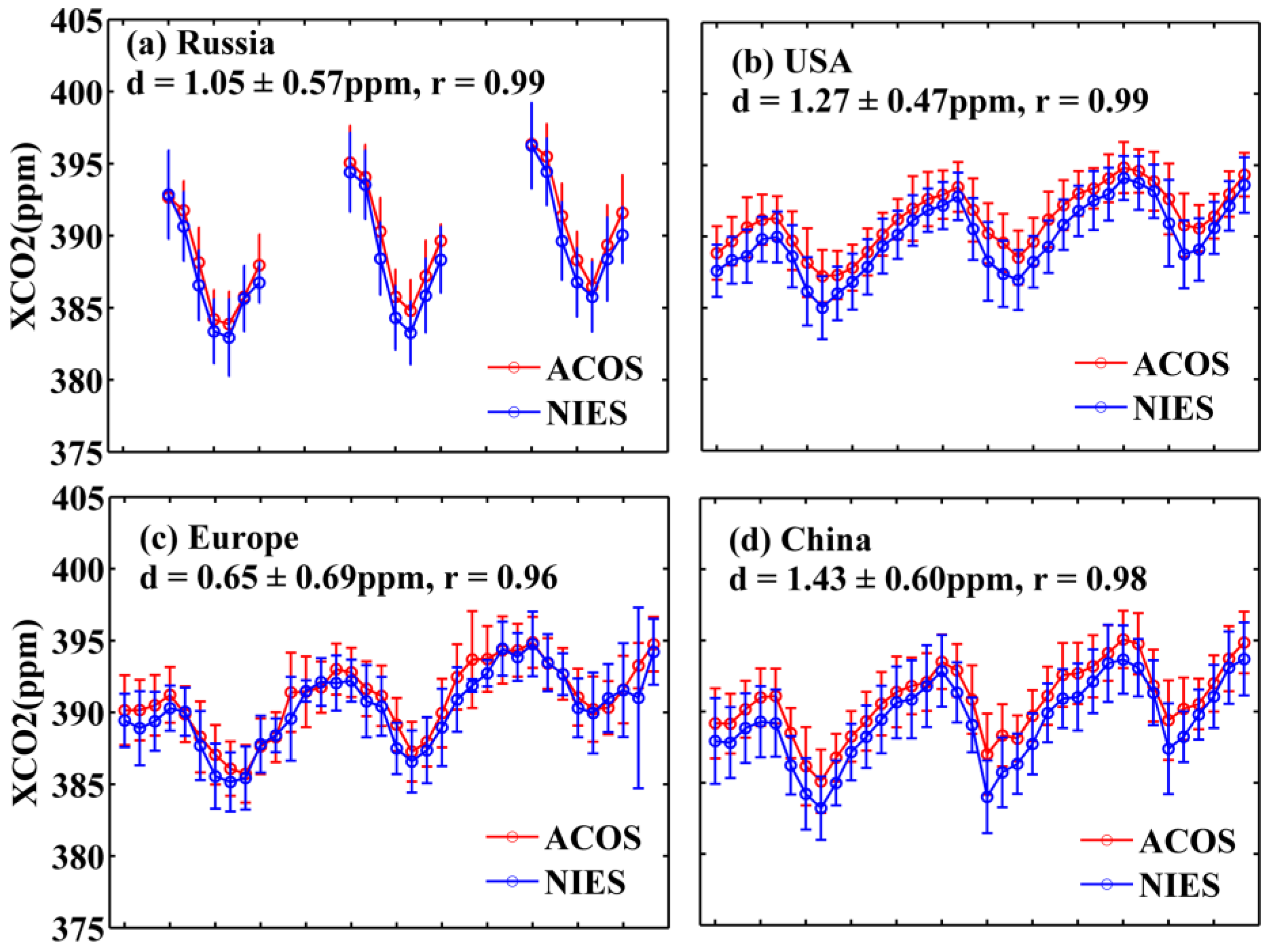
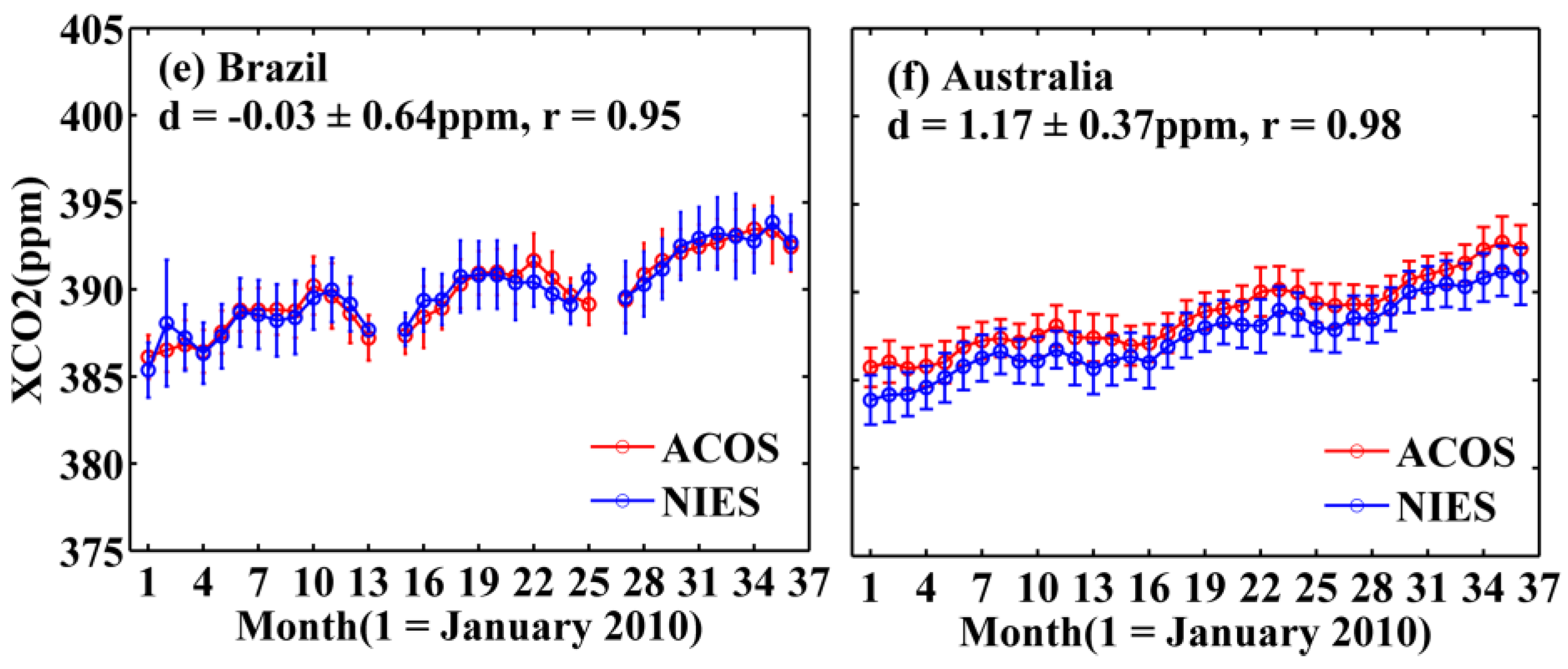
3.4. Comparison between ACOS and NIES XCO2 for Different Regions

Figure 6 shows the time series of XCO2 monthly means over Northern and Southern Hemisphere during the three years. Overall, good agreement is obtained for the monthly averages of NIES and ACOS XCO2 with respect to the amplitude and phase of XCO2 seasonal cycle. Compared with the Southern Hemisphere, the mean difference d of XCO2 monthly means over Northern Hemisphere is slightly larger (1.31 ± 0.64 ppm compared with 0.73 ± 0.34 ppm). In addition, the XCO2 seasonal fluctuation over Northern Hemisphere is significantly higher than Southern Hemisphere from both NIES and ACOS XCO2 monthly means. This is mainly because there is more land surface and the source/sink of CO2 is more obvious in Northern Hemisphere [30].
To further examine the difference between ACOS and NIES XCO2 for different regions, Figure 7 presents the XCO2 monthly means over six typical countries or regions. As can be seen from Figure 7, the differences of XCO2 monthly mean vary depending on the locations and months. Among the four northern countries or regions, the mean difference of XCO2 monthly means is smallest over Europe (0.65 ± 0.69 ppm) and the largest over China (1.43 ± 0.60 ppm). As there are large amounts of human activity and complex CO2 sources/sinks in China region, it may indicate large errors in the retrieval results for China region. In addition, the interference of high content and complex type of aerosol particles over China may also contribute to the difference between ACOS and NIES XCO2 retrievals. The mean difference is slightly larger for the USA (1.27 ± 0.47 ppm) than Russia (1.05 ± 0.57 ppm). In the Southern Hemisphere, the XCO2 monthly mean difference over Australia (1.17 ± 0.37 ppm) is significantly greater than that of Brazil (−0.03 ± 0.64 ppm).

4. Conclusions

The differences of ACOS and NIES GOSAT SWIR XCO2 datasets over High gain land surface for three years (2010–2012) were investigated in this paper. Since both NIES and ACOS XCO2 retrieval algorithms ingested GOSAT SWIR spectra and were based on the optimal estimation methods, good agreement was obtained for the CO2 global distribution, seasonal variation and monthly average time series between them. However, discrepancies still existed in the two XCO2 datasets. The yield of NIES XCO2 was about 71% of ACOS retrievals passing the recommended post-retrieval screening criteria. This was mainly ascribed to difference in the aerosol optical depth (AOD) filtering criteria and the solar zenith degree requirement between the two retrieval algorithms.
The overall XCO2 bias was 0.21 ± 1.85 ppm and −0.69 ± 2.13 ppm for ACOS and NIES, respectively, when compared with TCCON observations. The relative regional-scale accuracy was 0.62 and 0.93 ppm for ACOS and NIES. The ACOS XCO2 three-year means and seasonal means were generally greater than NIES by about 1 to 2 ppm. In addition, the mean differences between ACOS and NIES XCO2 monthly means varied over different regions with the largest difference over China (1.43 ± 0.60 ppm) and the least over Brazil (−0.03 ± 0.64 ppm). The differences in the handling of light scattering in the retrieval algorithms may lead to the difference in retrieval results. Furthermore, the bias correction applied to the ACOS XCO2 retrievals essentially reduced the global bias and enhanced the consistency with respect to TCCON data. The intercomparison between the two datasets indicates that ACOS XCO2 is globally higher than NIES by about 1 ppm and has a smaller bias and better consistency than NIES datasets.
This paper provides a reference for the evaluation of NIES and ACOS XCO2 retrieval algorithms and the suitability of the XCO2 products in applications. As can be seen, the ACOS XCO2 is generally higher than NIES retrievals. The difference between these two datasets is significantly large over the China region. It is suggested to further examine the difference of the two products from the aspects of approaches for retrieving cloud and aerosol optical properties, absorption spectroscopy of CO2 and oxygen (O2), as well as instrument characteristics.

Acknowledgments

This research was supported by the Major Special Project of the China High-Resolution Earth Observation System (NO: Y4D00100GF; 30-Y20A21-9003-15/17), Natural Science Foundation of China (No: 41371015, 41501401, and 41001207), and Youth Innovation Promotion Association of CAS (No: 2011062). We kindly thank the GOSAT team for providing the NIES GOSAT Level 2 data product. We also thank the ACOS/OCO-2 project for the ACOS Level 2 version 3.5 XCO2 product. TCCON data were obtained from the TCCON Data Archive, hosted by the Carbon Dioxide Information Analysis Center (CDIAC).

Author Contributions

Anjian Deng and Tianhai Cheng conceived and designed the experiments; Anjian Deng performed the experiments; Tianhai Cheng, Tao Yu, Xingfa Gu analyzed the data; Fengjie Zheng and Hong Guo helped perform the statistical analysis. Anjian Deng wrote the paper.

Conflicts of Interest

The authors declare no conflict of interest.

References

  1. World Data Centre for Greenhouse Gases. Available online: http://ds.data.jma.go.jp/gmd/wdcgg/pub/global/globalmean.html (accessed on 19 August 2016).
  2. Solomon, S.; Qin, D.; Manning, M.; Chen, Z.; Marquis, M.; Averyt, K.B.; Tignor, M.; Miller, H.L. Climate Change 2007: The Physical Science Basis, Contribution of Working Group 1 to the Fourth Assessment Report of the Intergovernmental Panel on Climate Change (IPCC); Cambridge University Press: Cambridge, UK, 2007. [Google Scholar]
  3. Gurney, K.R.; Law, R.M.; Denning, A.S.; Rayner, P.J.; Baker, D.; Bousquet, P.; Bruhwiler, L.; Chen, Y.-H.; Ciais, P.; Fan, S. Towards robust regional estimates of CO2 sources and sinks using atmospheric transport models. Nature 2002, 415, 626–629. [Google Scholar] [CrossRef] [PubMed]
  4. Stephens, B.B.; Gurney, K.R.; Tans, P.P.; Sweeney, C.; Peters, W.; Bruhwiler, L.; Ciais, P.; Ramonet, M.; Bousquet, P.; Nakazawa, T.; et al. Weak northern and strong tropical land carbon uptake from vertical profiles of atmospheric CO2. Science 2007, 316, 1732–1735. [Google Scholar] [CrossRef] [PubMed]
  5. Hungershoefer, K.; Breon, F.-M.; Peylin, P.; Chevallier, F.; Rayner, P.; Klonecki, A.; Houweling, S.; Marshall, J. Evaluation of various observing systems for the global monitoring of CO2 surface fluxes. Atmos. Chem. Phys. 2010, 10, 503–520. [Google Scholar] [CrossRef]
  6. Rayner, P.J.; O’Brien, D.M. The utility of remotely sensed CO2 concentration data in surface source inversions. Geophys. Res. Lett. 2001, 28, 175–178. [Google Scholar] [CrossRef]
  7. Houweling, S.; Breon, F.M.; Aben, I.; Rodenbeck, C.; Gloor, M.; Heimann, M.; Ciais, P. Inverse modeling of CO2 sources and sinks using satellite data: A synthetic inter-comparison of measurement techniques and their performance as a function of space and time. Atmos. Chem. Phys. 2004, 4, 523–538. [Google Scholar] [CrossRef] [Green Version]
  8. Miller, C.E.; Crisp, D.; DeCola, P.L.; Olsen, S.C.; Randerson, J.T.; Michalak, A.M.; Alkhaled, A.; Rayner, P. Precision requirements for space-based XCO2 data. J. Geophys. Res. 2007, 112, D10314. [Google Scholar] [CrossRef]
  9. Chevallier, F. Impact of correlated observation errors on inverted CO2 surface fluxes from OCO measuremtents. Geophys. Res. Lett. 2007, 34, L24804. [Google Scholar] [CrossRef]
  10. Yokota, T.; Yoshida, Y.; Eguchi, N.; Ota, Y.; Tanaka, T.; Watanabe, H.; Maksyutov, S. Global concentrations of CO2 and CH4 retrieved from GOSAT: First preliminary result. Sola 2009, 5, 160–163. [Google Scholar] [CrossRef]
  11. Yoshida, Y.; Ota, Y.; Eguchi, N.; Kikuchi, N.; Nobuta, K.; Tran, H.; Morino, I.; Yokota, T. Retrieval algorithm for CO2 and CH4 column abundances from short-wavelength infrared spectral observations by the Greenhouse gases observing satellite. Atmos. Meas. Tech. 2011, 4, 717–734. [Google Scholar] [CrossRef]
  12. Morino, I.; Uchino, O.; Inoue, M.; Yoshida, Y.; Yokota, T.; Wennberg, P.O.; Toon, G.C.; Wunch, D.; Roehl, C.M.; Notholt, J.; et al. Preliminary validation of column-averaged volume mixing rations of carbon dioxide and methane retrieved from GOSAT short-wavelength infrared spectra. Atmos. Meas. Tech. 2011, 4, 1061–1076. [Google Scholar] [CrossRef]
  13. Yoshida, Y.; Kikuchi, N.; Morino, I.; Uchhino, O.; Oshchepkov, S.; Bril, A.; Saeki, T.; Schutgens, N.; Toon, G.C.; Wunch, D.; et al. Improvement of the retrieval algorithm for GOSAT SWIR XCO2 and XCH4 and their validation using TCCON data. Atmos. Meas. Tech. 2013, 6, 1533–1547. [Google Scholar] [CrossRef]
  14. Wunch, D.; Wennberg, P.O.; Toon, G.C.; Connor, B.J.; Fisher, B.; Osterman, G.B.; Frankenberg, C.; Mandrake, L.; O’Dell, C.; Ahonen, P.; et al. A method for evaluating bias in global measurements of CO2 total columns from space. Atmos. Chem. Phys. 2011, 11, 20899–20946. [Google Scholar] [CrossRef]
  15. O’Dell, C.W.; Connor, B.; Boesch, H.; O’Brien, D.; Frankenberg, C.; Castano, R.; Christi, M.; Elderling, D.; Fisher, B.; Gunson, M.; et al. The ACOS retrieval algorithm—Part 1: Description and validation against synthetic observations. Atmos. Meas. Tech. 2012, 5, 99–121. [Google Scholar] [CrossRef]
  16. Crisp, D.; Fisher, B.M.; O’Dell, C.; Frankenberg, C.; Basilio, R.; Boesch, H.; Brown, L.R.; Castano, R.; Connor, B.; Deutscher, N.M.; et al. The ACOS CO2 retrieval algorithm-Part 2: Global XCO2 data characterization. Atmos. Meas. Tech. 2012, 5, 687–707. [Google Scholar] [CrossRef]
  17. Inoue, M.; Morino, I.; Uchino, O.; Miyamoto, Y.; Yoshida, Y.; Yokota, T.; Machida, T.; Sawa, Y.; Matsueda, H.; Sweeney, C.; et al. Validation of XCO2 derived from SWIR spectra of GOSAT TANSO-FTS with aircraft measurement data. Atmos. Chem. Phys. 2013, 13, 9771–9788. [Google Scholar] [CrossRef]
  18. Lei, L.P.; Guan, X.H.; Zeng, Z.C.; Zhang, B.; Ru, F.; Bu, R. A comparison of atmospheric CO2 concentration GOSAT-based observations and model simulations. Sci. China Earth Sci. 2014, 57, 1393–1402. [Google Scholar] [CrossRef]
  19. Goddard Earth Science Data Information and Services (GES DISC) of National Aeronautics and Space Administration (NASA). ACOS Level 2 Standard Production Data User’s Guide; v3.3; National Aeronautics and Space Administration: Washington, DC, USA, 2013.
  20. Zhang, H.F.; Chen, B.Z.; Xu, G.; Yan, J.W.; Che, M.L.; Chen, J.; Fang, S.F.; Lin, X.F.; Sun, S.B. Comparing simulated atmospheric carbon dioxide concentration with GOSAT retrievals. Chin. Sci. Bull. 2015, 60, 380–386. [Google Scholar] [CrossRef]
  21. Lindqvist, H.; O’Dell, C.W.; Basu, S.; Boesch, H.; Chevallier, F.; Deutscher, N.; Feng, L.; Fisher, B.; Hase, F.; Inoue, M.; et al. Does GOSAT capture the true seasonal cycle of carbon dioxide? Atmos. Chem. Phys. 2015, 15, 13023–13040. [Google Scholar] [CrossRef]
  22. Kulawik, S.; Wunch, D.; O’Dell, C.; Frankenberg, C.; Reuter, M.; Oda, T.; Chevallier, F.; Sherlock, V.; Buchwitz, M.; Osterman, G.; et al. Consistent evaluation of ACOS-GOSAT, BESD-SCIAMACHY, CarbonTracker, and MACC through comparisons to TCCON. Atmos. Meas. Tech. 2016, 9, 683–709. [Google Scholar] [CrossRef]
  23. Kuze, A.; Suto, H.; Nakajima, M.; Hamazaki, T. Thermal and near infrared sensor for carbon observation Fourier-transform spectrometer on greenhouse gases observing satellite for greenhouse gases monitoring. Appl. Opt. 2009, 48, 6716–6733. [Google Scholar] [CrossRef] [PubMed]
  24. Goddard Earth Science Data Information and Services (GES DISC) of National Aeronautics and Space Administration (NASA). ACOS Level 2 Standard Production Data User’s Guide; v3.5; National Aeronautics and Space Administration: Washington, DC, USA, 2016.
  25. Rodgers, C.D. Inverse Methods for Atmospheric Sounding: Theory and Practice; World Scientific: Singapore, 2000. [Google Scholar]
  26. Boesch, H.; Toon, G.C.; Sen, B.; Washenfelder, R.A.; Wennberg, P.O.; Buchwitz, M.; de Beek, R.; Burrows, J.P.; Crisp, D.; Christi, M.; et al. Space-based near-infrared CO2 measurements: Testing the Orbiting Carbon Observatory retrieval algorithm and validation concept using SCIAMACHY observations over Park Falls, Wisconsin. J. Geophys. Res. 2006, 111, D23303. [Google Scholar]
  27. Connor, B.J.; Boesch, H.; Toon, G.; Sen, B.; Miller, C.; Crsip, D. Orbiting carbon observatory: Inverse method and prospective error analysis. J. Geophys. Res. 2008, 113, D05305. [Google Scholar] [CrossRef]
  28. Wunch, D.; Toon, G.C.; Wennberg, P.O.; Wofsy, S.C.; Stephens, B.B.; Fischer, M.L.; Uchino, O.; Abshire, J.B.; Bernath, P.; Biraud, S.C.; et al. Calibration of the total carbon column observing network using aircraft profile data. Atmos. Meas. Tech. 2010, 3, 1351–1362. [Google Scholar] [CrossRef]
  29. Wunch, D.; Toon, G.C.; Blavier, J.F.L.; Washenfelder, R.A.; Notholt, J.; Connor, B.J.; Griffith, D.W.T.; Sherlock, V.; Wennberg, P.O. The total carbon column observing network. Philos. Trans. R. Soc. A 2011, 369, 2087–2112. [Google Scholar] [CrossRef] [PubMed]
  30. Schneising, O.; Buchwitz, M.; Reuter, M.; Heymann, J.; Bovensmann, H.; Burrows, J.P. Long-term analysis of carbon dioxide and methane column-averaged mole fractions retrieved from SCIAMACHY. Atmos. Chem. Phys. 2011, 11, 2863–2880. [Google Scholar] [CrossRef]
Figure 1. The column averaged dry air mole fractions of atmospheric carbon dioxide (XCO2) bias (a) and standard deviation (b) of the Atmospheric CO2 Observations from Space (ACOS) and the National Institute for Environmental Studies (NIES) versus Total Carbon Column Observing Network (TCCON) observations listed in Table 1. The TCCON sites are arranged from high to low latitude.
Atmosphere 07 00109 g001
Figure 2. Histogram of the difference of ACOS relative to TCCON (a) and NIES relative to TCCON (b) for all TCCON sites listed in Table 1.
Atmosphere 07 00109 g002
Figure 3. The monthly number time series of global retrieved NIES and ACOS XCO2 passing the post-screening filters. The data is limited to High gain land surface.
Atmosphere 07 00109 g003
Figure 4. Global distribution of three-year averages of ACOS (a) and NIES (b) XCO2 and their difference (c) gridded in 2.5° × 2.5° bins from 2010 to 2012; the histogram of difference shown in (c) is presented in (d).
Atmosphere 07 00109 g004
Figure 5. Seasonal difference (a) gridded in 2.5° × 2.5° bins between ACOS and NIES XCO2 means and the histogram of their difference (b) in each season from December 2011 to November 2012.
Atmosphere 07 00109 g005
Figure 6. Time series of NIES and ACOS XCO2 monthly mean in the Northern (a) and Southern (b) Hemispheres for three years. The mean difference d of ACOS to NIES and its corresponding standard deviation, and the correlation coefficient r between NIES and ACOS are evaluated based on the XCO2 monthly means.
Atmosphere 07 00109 g006
Figure 7. The same as Figure 6 but for six countries or regions. There are some XCO2 monthly means unavailable over Russia and Brazil.
Atmosphere 07 00109 g007aAtmosphere 07 00109 g007b
Table 1. Summary of comparison of ACOS and NIES XCO2 versus TCCON observations. Shown are the coincided number n between satellite retrievals and TCCON data, the mean difference d (station bias) and standard deviation std of their difference, and the correlation coefficients r. The global offset, which is averaged d, the regional precision, which is averaged std, the relative accuracy, which is a standard deviation of d, and the mean correlation, which is averaged r, are also given at the bottom of the table.
SitesACOS—TCCONNIES—TCCON
nd (ppm)std (ppm)rnd (ppm)std (ppm)r
Sodankyla (67.37°N, 26.63°E)501.541.470.9145−0.911.930.89
Bialystok (53.23°N, 23.02°E)93−0.061.570.8823−0.221.840.78
Bremen (53.10°N, 8.85°E)440.551.840.827−0.811.580.66
Karlsruhe (49.1°N, 8.44°E)1311.282.560.62100.531.140.85
Orleans (47.97°N, 2.11°E)2030.031.950.7532−0.402.220.48
Garmisch(47.48°N,11.06°E)2121.072.180.75221.092.440.74
Park Falls (45.94°N, 90.27°W)2390.222.080.841300.461.940.85
Lamont (36.6°N, 97.49°W)1170−0.231.430.8827−1.491.520.87
JPL, Pasadena (34.2°N, 118.18°W)267−0.492.280.69111−2.352.470.68
Darwin (12.43°S, 130.89°E)2810.781.210.6185−0.591.290.36
Wollongong (34.41°S, 150.88°E)5080.561.910.6336−0.911.090.88
Lauder (45.04°S, 169.68°E)1260.341.620.7770−0.781.650.76
Global offset (ppm)0.47−0.53
Regional precision (ppm)1.841.76
Relative accuracy (ppm)0.620.93
Mean correlation0.760.73

