Comparison of Ozone Production Regimes between Two Mexican Cities: Guadalajara and Mexico City

Abstract

Ozone concentrations have been increasing in the Guadalajara Metropolitan Area (GMA) in Mexico. To help devise efficient mitigation measures, we investigated the ozone formation regime by a chemical transport model (CTM) system WRF-CMAQ. The CTM system was validated by field measurement data of ground-level volatile organic compounds (VOC) and vertical profiles of ozone in GMA as well as in the Mexico City Metropolitan Area (MCMA). By conducting CTM simulations with modified emission rates of VOC and nitrogen oxides (NO_x), the ozone formation regime in GMA was found to lie between VOC-sensitive and NO_x-sensitive regimes. The result is consistent with the relatively large VOC/NO_x emission ratio in GMA compared to that in MCMA where the ozone formation regime is in the VOC-sensitive regime.

1. Introduction

Guadalajara and the surrounding cities constitute Guadalajara Metropolitan Area (GMA), the second largest Mexican metropolitan area next to Mexico City Metropolitan Area (MCMA). Although air quality in MCMA has improved considerably since its worst times around 1990, that in GMA shows worsening tendency especially in ozone (O₃) concentration that has been increasing recently [1]. To curb the trend, we need to understand the current photochemical state of the GMA lower troposphere.

In contrast to the air pollution in GMA, that in MCMA has been studied extensively, and the mechanism of pollution generation, especially in the gas phase, has been understood fairly well. For O₃, the formation has been determined to be in the VOC-sensitive regime [2] where an increase of VOC (Volatile Organic Compounds) leads to an increase of O₃ while an increase of NO_x (nitric oxide (NO) and nitrogen dioxide (NO₂)) leads to a decrease of O₃ [3]. The VOC-sensitive regime occurs in an atmosphere with a relatively small emission of VOC compared to that of NO_x, a state commonly found in densely populated cities [4,5] unless extended VOC sources such as natural vegetation exist in the neighborhood (e.g., Atlanta, GA, USA, [6]).

There have been only a small number of studies on the atmospheric environment of GMA. Ramirez-Sanchez et al. [7] analyzed the continuous measurement data from 2000 to 2005 of criteria air pollutants (carbon monoxide (CO), NO₂, sulfur dioxide (SO₂), O₃, and PM₁₀ (particulate matter with aerodynamic diameter less than 10 $\mathsf{\mu }$m)) at eight monitoring stations. Although high variability existed, it was found that the Mexican air-quality standards were exceeded for a quarter to half the days of the year. For O₃ that is of primary concern in this paper, the Mexican standard is 110 ppb for one-hour average and 80 ppb for 8-h average, higher than 60 ppb in Japan for one-hour average, 75 ppb and 120 $\mathsf{\mu }$g·m⁻³ (61 ppb for 1013 hPa and 25 °C) in EU for 8-h average. Comparison of air-quality standards for other pollutants can be found in Benitez-Garcia et al. [1]. Benitez-Garcia et al. [1] analyzed the air-quality monitoring data in MCMA, GMA, and Monterrey Metropolitan Area (MMA) from 2000 to 2011. In GMA and MMA, both the annual mean and the 98th-percentile values of daily averaged O₃ concentrations exhibited increasing trends whereas those in MCMA were decreasing. Specifically, the annual average concentration of O₃ in GMA increased by 47% from 2000 to 2011, and the number of days when the Mexican air-quality standard for the hourly average was exceeded at the Centro monitoring station (CEN) increased from 10–30 in the early 2000s to 30–40 in the late 2000s. For NO₂, no clear trend of the annual mean concentration was discernible due to the low data validity in the late 2000s, but the annual 98th-percentile value decreased from about 0.5 ppm in the early 2000s to 0.2 ppm in the late 2000s. Concerning O₃ formation, Jaimes-Lopez et al. [8] investigated using a smog chamber the effect of adding or removing VOC species in the sampled ambient air of MCMA and GMA. They found that removing half the amount of total non-methane hydrocarbons resulted in greater reduction of O₃ than removing only components of liquefied petroleum gas (LPG). Their results are consistent with the low OH-reactivity of LPG components, mostly propane and butane. Mendoza and Garcia [9] applied an Eulerian photochemical air quality model: CIT airshed model [10]. For a period from 16 to 18 May 2001, they obtained an acceptable agreement with the ground-level monitoring data. Using the same model in an iterative manner, they modified the emissions inventory to improve the model performance [11]. Other modeling studies exist that are based on a statistical method [12] or a neural-network method [13]. These studies might be useful for prognosis purposes under the assumption that the current climate or emission condition will remain unchanged. However, to develop effective mitigation measures, methods based on physical and chemical mechanisms are required.

In this study, field measurement campaigns were conducted in GMA to obtain the detailed atmospheric chemical composition. In addition to regular measurement of criteria pollutants at air-monitoring stations, vertical distribution of O₃ concentration was measured by ozonesonde, and concentrations of VOC species were obtained by analysis of canister samples. Chemical transport model (CTM) simulations were conducted using Community Multiscale Air Quality (CMAQ) modeling system [14], a more advanced model than the above-mentioned CIT airshed model developed in the early 1980s. The CMAQ simulations validated by the field observation data were used to determine the O₃ formation regime. Where appropriate, comparison with MCMA is presented to clarify the characteristics of GMA.

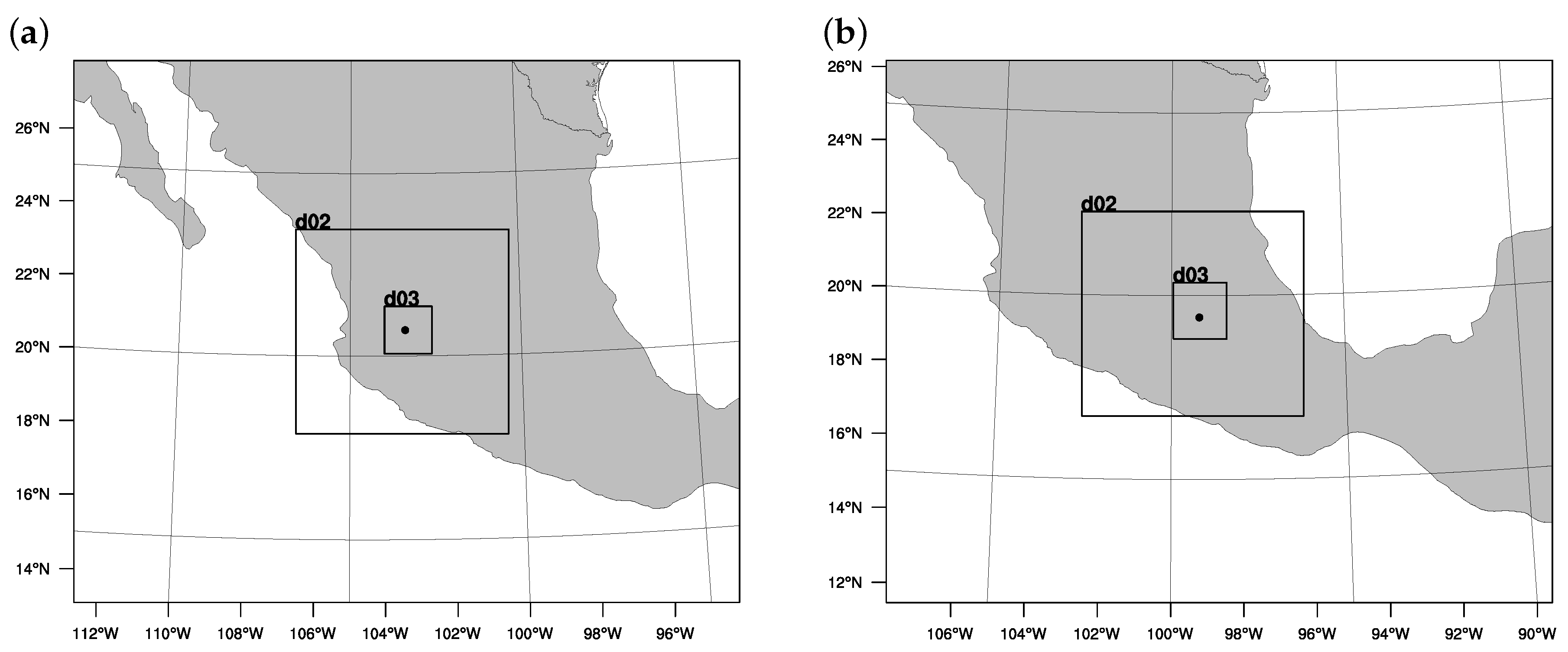
2. Geography and Climate

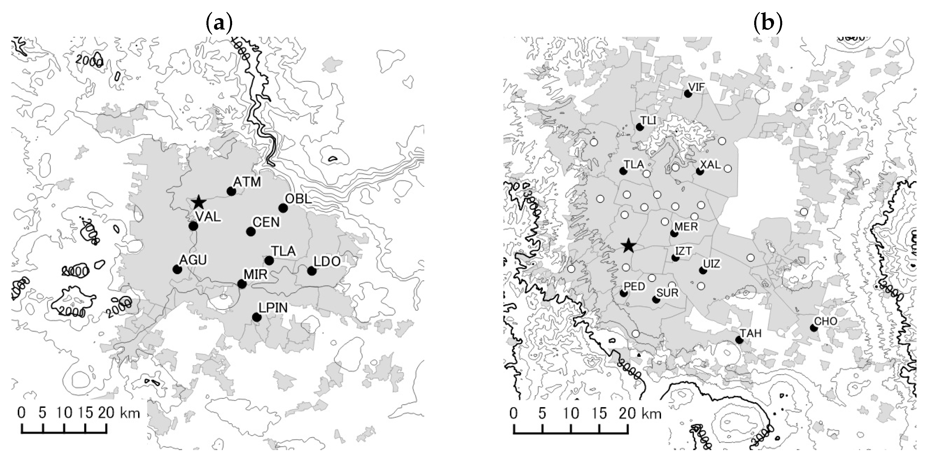
Figure 1 shows the maps of GMA and MCMA.

GMA belongs to the temperate humid subtropical climate (C_wa by the Köppen–Geiger classification) with dry winter and wet summer. The mean elevation is 1540 m above sea level (a.s.l.). The urban core of GMA is bordered by the Primavera Forest (about 2000 m a.s.l.) on the west side and a valley of Rio Grande de Santiago (about 500 m deep) on the northeast side. The prevailing wind in GMA is the westerly sea breeze coming from the Pacific ocean about 230 km to the west.

The population in GMA is about 4 million. The primary economic activity in GMA is commerce. In GMA, there are not many factories of heavy industries, and most air pollutants are emitted from automobiles. Because there is no exhaust-gas inspection scheme in GMA, proportions of old cars are much higher than in MCMA where strict regulations are implemented [1].

MCMA belongs to the temperate highland tropical climate (C_wb by the Köppen–Geiger classification) with dry winter and wet summer as in GMA. The mean elevation is 2240 m a.s.l. The urban core of MCMA is surrounded by mountain ranges on the west, east, and southwest sides. There is a wide opening to the north and a narrow one to the southeast. The local wind circulation is governed by the updraft above the heated basin and convergence from the surrounding lower altitudes that brings adiabatically expanded cool air into the basin [15]. The prevailing wind in MCMA is northerly.

The population in MCMA is 20 million. The main economic activity is commerce. Many of the heavy-industry factories have been relocated out of the Mexico City basin since the worst air-pollution periods around 1990. As in GMA, the largest source of air pollutants is the automobile. Although the number of registered vehicles in MCMA is more than four times than that in GMA, the strictly enforced exhaust-gas regulations suppress the emission per vehicle (described in Section 4.1).

3. Field Data

In both GMA and MCMA, intensive field measurement campaigns were conducted to investigate the formation mechanisms of O₃ and PM_2.5 (particulate matter with aerodynamic diameter less than 2.5 $\mathsf{\mu }$m). Field measurements related to this paper were ozonesonde for vertical profiling of O₃ concentration and VOC analysis of canister samples using gas chromatography (GC).

The MCMA campaign conducted in March 2012 has already been reported for ozonesonde [16,17] and VOC analysis [18]. The O₃-concentration profiles obtained twice daily in the morning and afternoon reflected the meteorological condition on the observation days [17]. It is noteworthy that SO₂ emitted from an active volcano in the southeast and an industrial complex in the north interfered the ozonesonde measurement in MCMA [16]. The VOC analysis by GC with flame ionization detector (FID) and mass spectrometer (MS) confirmed previous findings such as that a large proportion of VOC was LPG related to domestic consumption and that more reactive and toxic species than the LPG components could be attributed to vehicular transport and solvent-related industries [18].

In MCMA, VOC concentrations were obtained from a concurrent campaign conducted by the government of the Federal District (GDF by Spanish acronym) [19]. Two of the measurement sites (Pedregal (PED) and Merced (MER); see Figure 1b) coincided with those of the campaign mentioned above. Non-methane hydrocarbons (C2-C12) were measured using an on-line Syntech Spectras system model GC955 611/811 (Synspec BV, Groningen, Netherlands). To cover the range of hydrocarbons C2-C12, this instrument is designed like a double GC, one for C2-C5 and the other for C6-C12. The accuracy of the instrument was maintained within ±10% through a multipoint calibration using a standard gas mixture. The measurement had a time resolution of 30 min. Because of the time resolution, the GDF dataset was more appropriate for comparison with numerical simulation than that of the canister samples (3 or 24 h).

The GMA campaigns were conducted in May 2012 and May 2014. Because an approaching hurricane during the campaign of May 2012 made the atmosphere not representative of the typical fair weather condition, we will use the data only from the latter campaign conducted from 5 to 9 May 2014. Ozonesonde and radiosonde were launched from the meteorological observatory (20.7067°N, 103.3925°W, 1559 m a.s.l.) located in a large park (the star symbol in Figure 1a). The ozonesonde was launched at 10:30 local standard time (LST) (16:30 UTC), 13:30 LST (19:30 UTC), and 16:00 or 16:30 LST (22:00 or 22:30 UTC). Radiosonde for the measurement of temperature, humidity, and wind components was launched at 7:30 LST (13:30 UTC) and 16:30 (22:30 UTC). Note that daylight saving time (DST) was in effect during the campaign so that LST was one hour behind DST. The launches were canceled because of rain in the afternoon of 7 May 2014, and all day on 8 May 2014. The measurement devices were the same as in the MCMA campaign [16,17], i.e., RS-06G (Meisei Electric Co. Ltd., Isezaki, Japan) for radiosonde and electrochemical concentration cell (ECC) sensor (EnSci Co., Westminster, CO, USA) attached to RS-06G for ozonesonde. At about 1.5 m above the ground, the output of the ECC sensor of the ozonesonde was confirmed to agree within 5 ppb with a UV-absorption-based monitor (OA-781, Kimoto Electric, Japan) that was calibrated against the Standard Reference Photometer #39. The accuracy of ECC sensors of the same type is reported to be $\pm 6$% near the ground, and −7% to +17% in the high troposphere [20].

For VOC measurement in the GMA campaign, the ambient air was sampled by canisters at the CEN station (see Figure 1a) on 5, 6, and 7 May 2014. The sampling duration of each canister was 3 h, and eight samples per day were obtained. Twenty-four-hour samples were also collected on 5 and 8 May 2014. The canister samples were analyzed for the concentrations of VOC species by GC-FID and GC-MS by the same method as in MCMA [18]. The GC-FID and GC-MS systems were calibrated against certified standard gas mixtures with ±10% accuracy. No automated continuous measurement was conducted during the GMA campaign.

In addition to the campaign data, hourly monitoring data of criteria air pollutants were obtained from the web pages of the Jalisco state government for GMA and those of GDF for MCMA. The monitoring instruments were calibrated by the US-EPA protocols.

4. Chemical Transport Simulation

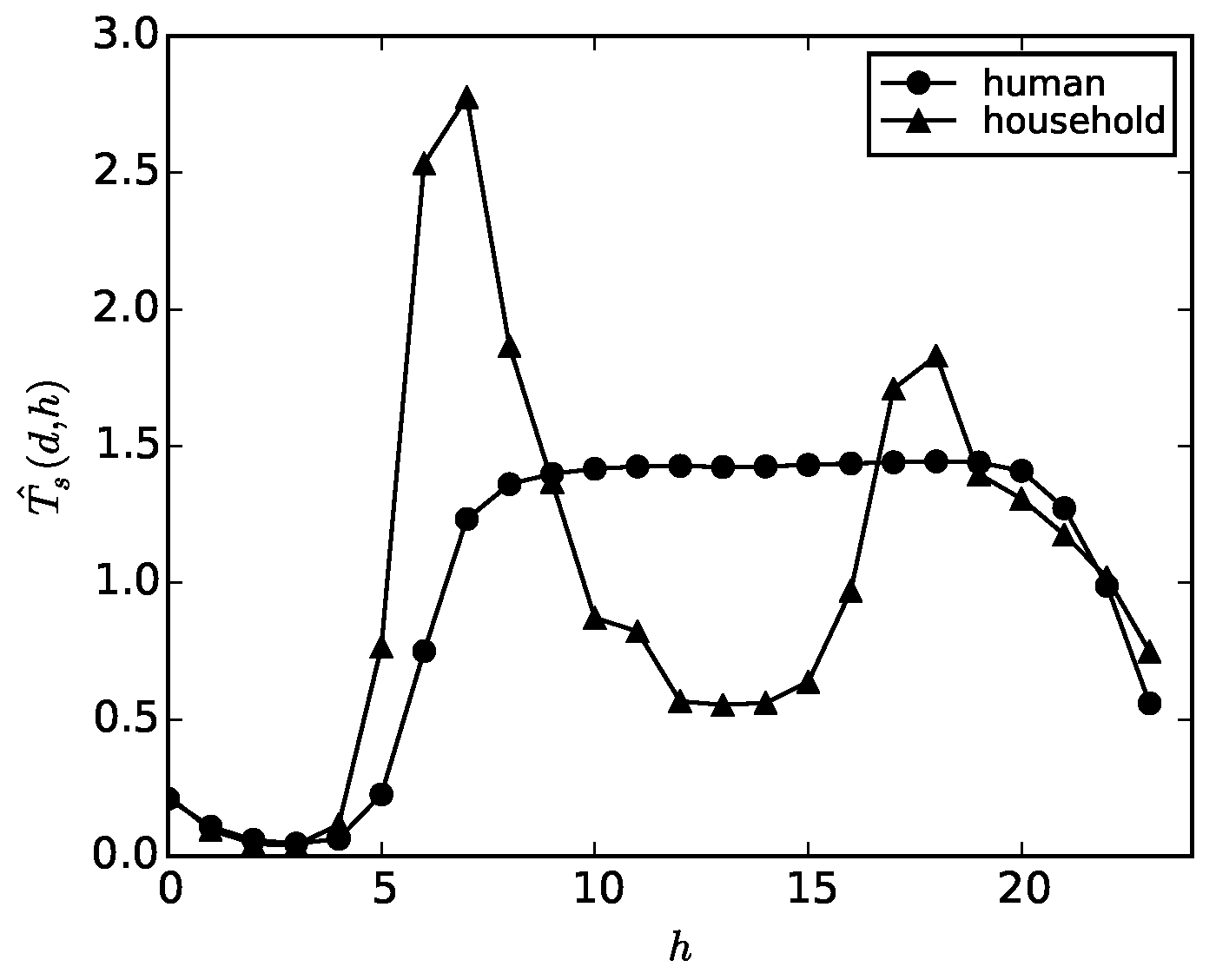
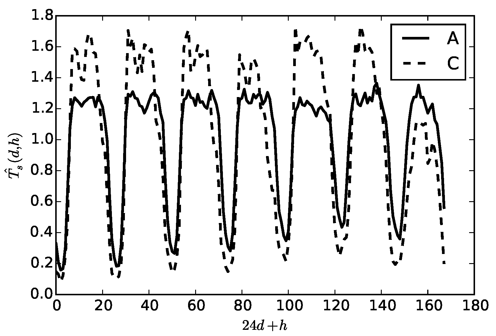
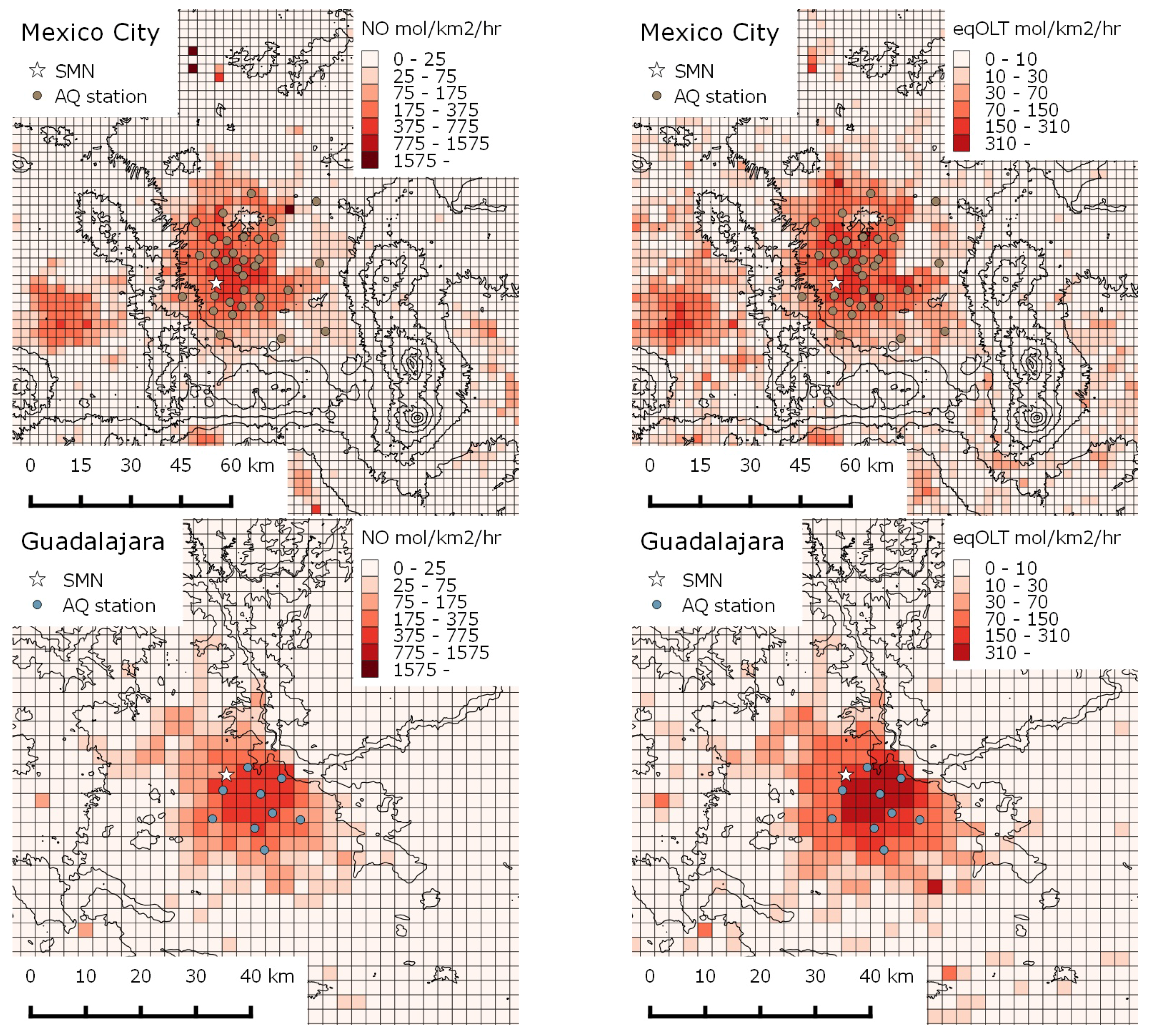
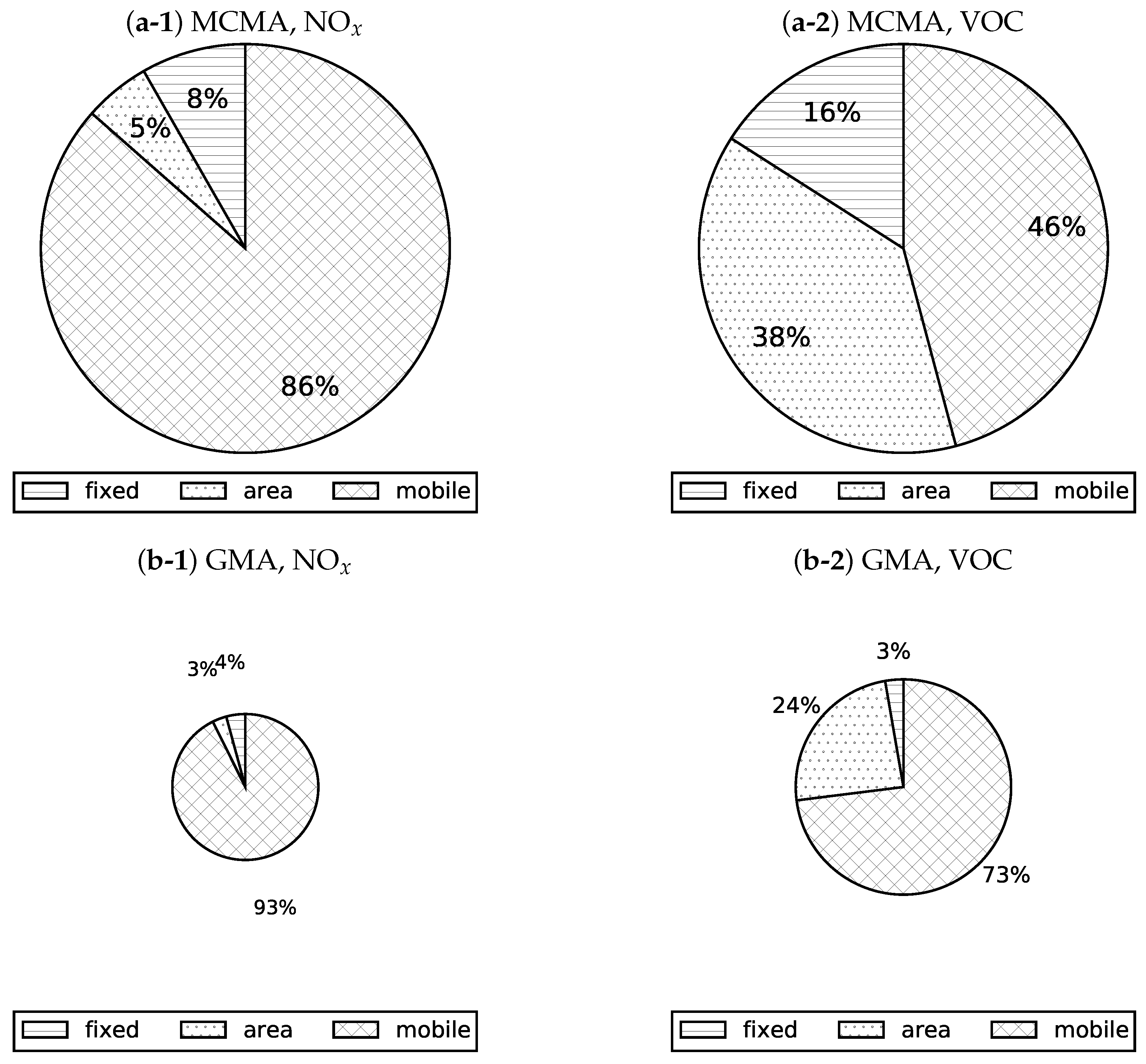
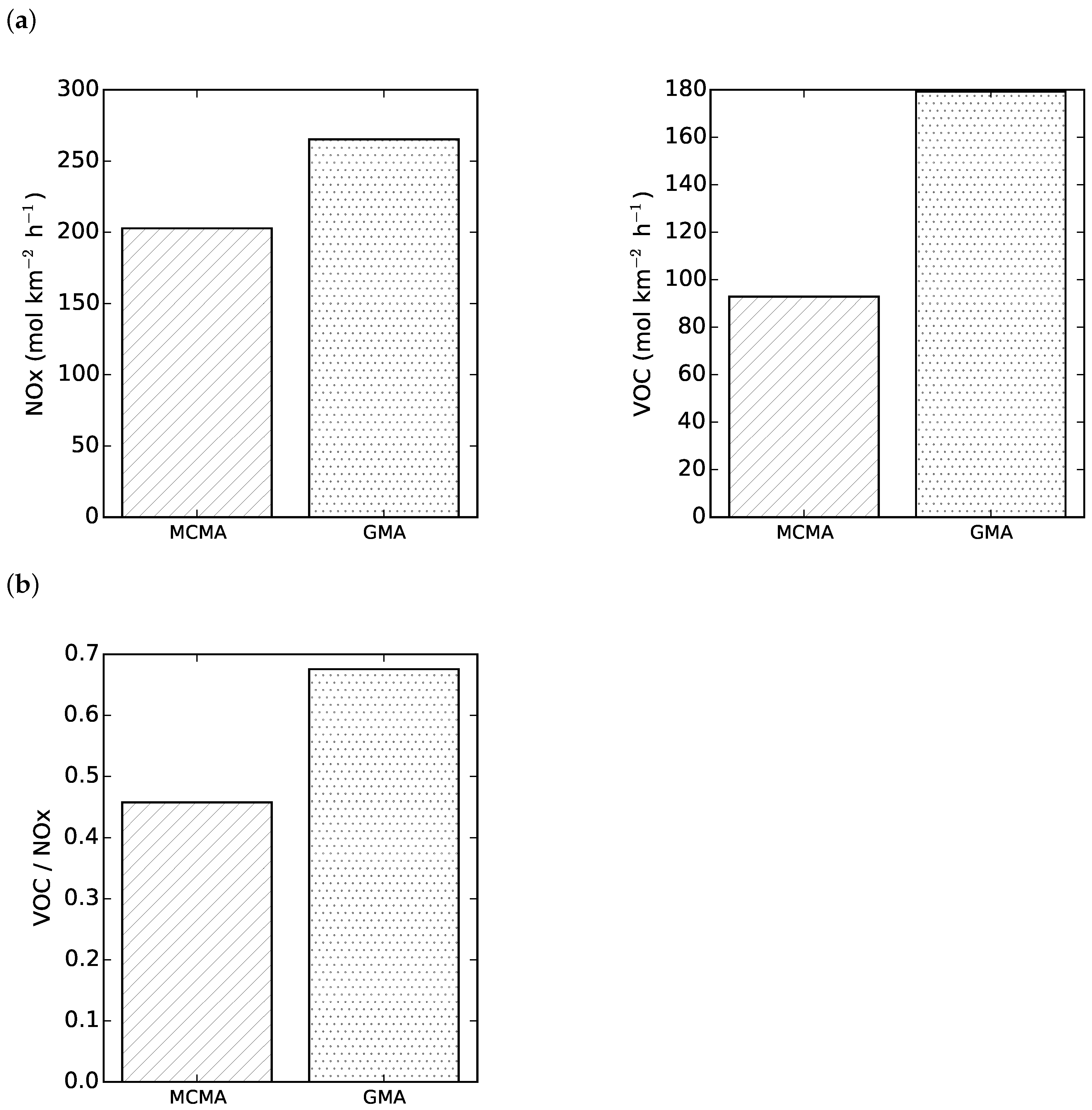
4.1. Emissions Data

CTM simulations require emissions data allocated on the simulation grid. Gridded anthropogenic emissions in MCMA and GMA were constructed from the latest available national emissions inventory Inventario Nacional de Emisiones de Mexico 2008 (INEM2008) compiled by Secretary of Environment and Natural Resources (SEMARNAT by Spanish acronym). INEM2008 classifies anthropogenic emission sources into fixed, area, and mobile types. The emission species are CO, NO_x, SO₂, VOC, ammonia, black carbon, PM₁₀, and PM_2.5.

For fixed sources, INEM2008 lists longitude-latitude locations, operation hours, and stack properties of individual factories. Annual emissions are given for different processes of each factory. Area sources are further classified into sub-categories such as car-painting solvent usage and domestic LPG leakage. Annual emissions are provided for each sub-category in each municipality. Mobile sources are classified into the railway, marine, construction, agriculture, aviation, airport, and road. The road mobile sources are further classified by model year and vehicle types such as light-duty gasoline vehicle and heavy-duty diesel vehicle. For each sub-category, annual emissions are given in each municipality.

The emission data were redistributed onto regular grids of 0.025° intervals in both longitude and latitude, and 20-m interval in the vertical. The fixed emissions were assigned to the grid cells that include the source locations. Stack emissions were allocated to the cells where the tops of stacks lied, emissions from ground-level processes were allocated to the lowest layer with a thickness of 20-m, which is comparable to the lowest layer thickness 26 m of the WRF-CMAQ simulation.

The area emissions were weighted by population or landuse depending on the source type (e.g., population-weighting for domestic use of aerosol products, and landuse-weighting for solvent usage in the industrial coating). The population data as of 2010 were extracted from a geographical information system (GIS) software MAPA DIGITAL v.5 developed by the Mexican National Institute of Statistics and Geography (INEGI by Spanish acronym). The landuse data were downloaded from an INEGI website [21]. All the area emissions were allocated to the lowest layer.

For mobile emissions, airport and aviation categories were allocated to the airport area. Construction and agricultural categories were distributed by landuse. The railway and marine categories were omitted because they are not important sources in MCMA and GMA and also because GIS data for proper emission distribution were not readily available. Road emissions were distributed in proportion to the effective road length in each grid cell. Road network dataset was constructed by combining three databases: “Red Nacional de Caminos” [21], “Carreteras Vialidades Urbanas” [21], and OpenStreetMap [22]. It was assumed that federal and state roads emit four times more pollutants than other roads. This crude estimate based on visual inspection of the urban traffic does not affect the resulting emissions distribution considerably because the grid resolution 0.025° (about 2.8 km in the latitudinal direction) is relatively coarse. All the mobile emissions were allocated to the lowest layer.

Given an annual emission E, the hourly emission e was calculated by

$$e={\widehat{T}}_s(d,h)\frac{E}{365\times 24}$$

(1)

where d (0 = Monday, ⋯, 6 = Sunday) denotes day of the week and h denotes hour of the day. The activity coefficient ${\widehat{T}}_s(d,h)$ satisfies

$$\frac{1}{7\times 24}\sum _{d=0}^6\sum _{h=0}^{23}{\widehat{T}}_s(d,h)=1$$

(2)

Dependence on the month was not considered because the seasonal variation of monthly mean temperature is relatively small (about 5 °C in MCMA and 8 °C in GMA), and heating in winter is not common in MCMA and GMA.

For fixed sources, emissions were allocated uniformly during the operation hours. For area sources, different temporal patterns of daily activity were assumed for different groups of sub-categories. Figure 2 shows “human” and “household” patterns derived from a Japanese survey [23]. It was assumed that the daily life cycle is the same in Japan and Mexico. For example, domestic solvent usage was distributed by the “human” pattern, and domestic LPG combustion was distributed by the “household” pattern. For construction and agricultural mobile sources, emissions were allocated uniformly to typical working hours: 7:00–17:00 LST for agriculture and 8:00–17:00 LST with a lunch break in 13:00–14:00 LST for construction. For airport and aviation, emissions were distributed in proportion to the number of arrivals and departures listed on published timetables. For road mobile sources, mean temporal patterns for passenger cars and trucks derived from a traffic census in 2003 in MCMA (provided by GDF through institutional agreement) were adopted for ${\widehat{T}}_s(d,h)$. In the traffic census, 30 master stations were set up where the passing vehicles were counted by a pneumatic-tube system. Average temporal patterns of the traffic flow rate were determined from the 11 stations where the data quality was good. Figure 3 shows the patterns beginning at 0:00 LST Monday. The following features are noted: (1) passenger cars (A) have less day-night variation than trucks (C); (2) daytime traffic is clearly less on Sunday, but not on Saturday; (3) daytime truck traffic is less on Thursday; and (4) nighttime traffic increases monotonically from Sunday to Friday. The last feature is peculiar to Mexico where many people go outside on Friday nights.

In GMA than in MCMA, people tend to drive shorter distances at higher speed from later in the morning to earlier in the evening because of the less intense commuter traffic. However, because there were no comparable traffic census data in GMA, the same temporal patterns as in MCMA were applied to GMA.

VOC and NO_x were speciated into component species in the following manner. VOC was speciated in two steps: (1) division into chemical compounds based on the category-specific profiles defined in SPECIATE v4.4 [24]; and (2) aggregation into chemical mechanism species based on Carter’s tables [25]. In the second step, either RADM2 or SAPRC99 was adopted as the chemical mechanism. RADM2 that groups together compounds based on OH-reactivity was used for calculating effective VOC emission rates weighted by OH-reactivity. SAPRC99 was used for the CMAQ simulation, which by default does not work with RADM2. NO_x was divided into NO and NO₂ using the NO/NO_x ratio derived from a report on a Japanese emissions inventory [26]. Note that the NO/NO_x ratio for diesel vehicles was set to 0.9, which is appropriate for Japanese diesel vehicles not equipped with devices for reducing exhaust of particulate matter.

For the reason discussed in Section 4.3, emissions from the road mobile source were modified by multiplying a factor 0.6 uniformly on all the species. All the results presented in this paper were obtained using the modified road mobile emissions.

Figure 4 shows the gridded distributions of emission intensities of NO and the effective VOC summed over the vertical layers. The effective VOC was defined as the total molar amount of VOC species weighted by the reaction rate with OH radical (OH-reactivity) relative to that of OLT (terminal olefin such as propene) in RADM2. Note that, in generating Figure 4, ${\widehat{T}}_s(d,h)$ was temporarily set unity for all d and h to show time-averaged distributions. We observe that strong emission is concentrated around the city center, reflecting the high contribution of mobile sources. It should be noted that, in MCMA, there is a factory with an extremely large emission of VOC outside the urban core of MCMA. Considering that the O₃ concentration at a monitoring station downwind of this plant do not exhibit any particularly high values whereas CTM simulations using the default emissions predicted distinctly high O₃ concentration at this station, we suspect that the default emission value for this factory is faulty. However, due to the contract with industries, we are not permitted to describe the specific location, emission amount, or how much the actual proportion of the fixed source would become without this factory. Because the effect of this factory in the CTM simulation was limited to outside the urban core of MCMA, we decided to leave the large emission as in the default INEM2008. In the comparison between CTM and observation (Section 4.3), the monitoring station that was affected substantially was excluded.

Figure 5 shows the proportions of NO_x and OLT-equivalent VOC emissions among fixed, area, and mobile sources. The emissions were summed over the grid cells where more than half the cell area is categorized as urban landuse. Both in MCMA and GMA, mobile sources dominate the NO_x emission. For VOC, the mobile sources occupy nearly half in MCMA and two-thirds in GMA. Because of the suspiciously large emission from a factory mentioned previously, the relatively large proportion of VOC for the fixed sources in MCMA may be much smaller in reality.

The emission ratio of VOC and NO_x is a major factor affecting the O₃ formation regime. Figure 6 shows the emission rates of NO_x and OLT-equivalent VOC in the urban grid cells of MCMA and GMA. Although the total values are greater in MCMA than in GMA, the averaged values per unit area (Figure 6a) are greater in GMA than in MCMA. It should be remarked that the officially defined metropolitan areas include considerable expanses of non-urban landuse areas. The whole areas of MCMA and GMA are 7900 and 2760 km², respectively, much greater than the urban landuse areas (2061 km² in MCMA and 562 km² in GMA). Because the emission rate of VOC is relatively high in GMA, the ratio VOC/NO_x becomes distinctly higher in GMA than in MCMA (Figure 6b).

4.2. Simulation Model

To determine the O₃ production regime in GMA, we conducted CTM simulations using CMAQ combined with Weather Research and Forecasting (WRF) model [27] for reproducing the meteorological field. The versions used were 3.6 for WRF and 5.0.2 for CMAQ. Salient simulation parameters are listed in

Table 1. Parameters for the WRF simulation.

Nesting	triple (d01, d02, and d03 from coarser to finer domain)
Grid Size	27 – 9 – 3 km
Vertical Layers	31 layers up to 50 hPa
Shortwave Radiation	Goddard scheme
Longwave Radiation	RRTM scheme
Microphysics	Lin et al. scheme
Planetary Boundary Layer	YSU scheme
Surface Layer	Revised MM5 Monin–Obukhov scheme
Landuse	unified Noah LSM
Urban Canopy Model	d03 only
Cumulus Clouds	Grell-3 scheme (d01, d02 only)
Boundary Condition	NCEP FNL (d01 only)
Grid Nudging	NCEP FNL (d01 only)

and

Table 2. Parameters for the CMAQ simulation.

Chemical Mechanism	SAPRC99
Radiation	table (off-line)
Emission	EDGAR v4.2 + MEGAN v2.10 (d01,d02)
	INEM2008 + MEGAN v2.10 (d03)
Boundary Condition	MOZART-4/GEOS-5 (d01)
Initial Condition	d01: Default profile
	d02: End state of the first day of d01
	d03: End state of the second day of d02

. The WRF simulation nests are shown in Figure 7. The simulation periods were from 25 February 2012 to 15 March 2012 for MCMA, and from 23 April 2014 to 10 May 2014 for GMA. Counting from the third simulation day when the CMAQ calculation for the inner-most domain (d03) began, the first ozonesonde observation days (7 March 2012 in MCMA, and 5 May 2014 in GMA) correspond to the 10th and 11th day, respectively, for MCMA and GMA. The anthropogenic emission based on INEM2008 was applied on the basis of LST in MCMA and DST in GMA. Natural emissions including biogenic VOCs were modeled by the Model of Emissions of Gases and Aerosols from Nature (MEGAN) v2.1 [28] in all the simulation nests. MEGAN v2.1 generated speciated natural emissions from the databases of leaf area index, plant functional type, and emission factors at a 30-arc-second spatial resolution for the base year 2008. The emission rates at each hour were calculated under the WRF-simulated meteorological condition and were aggregated in the CTM simulation cells.

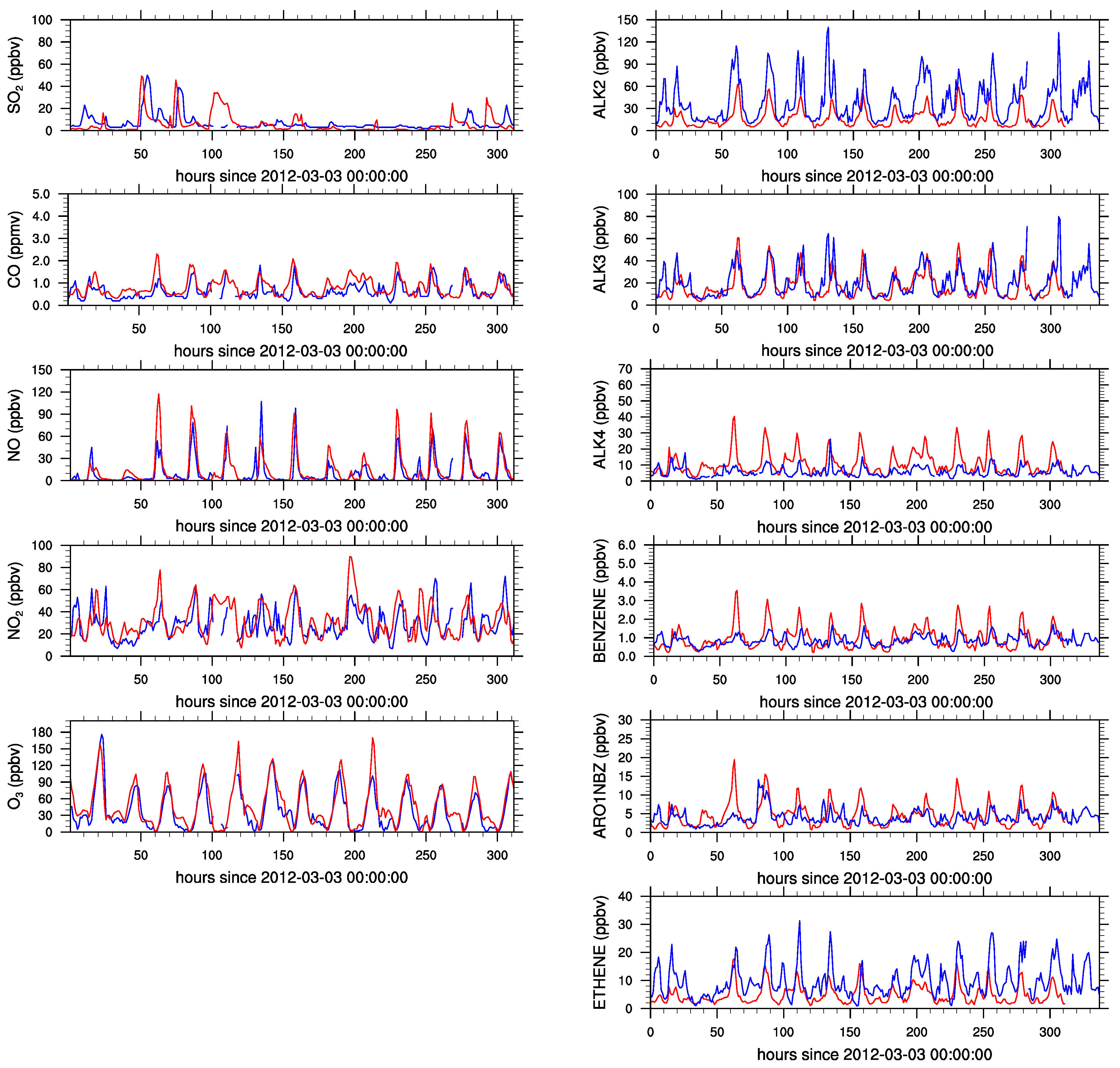
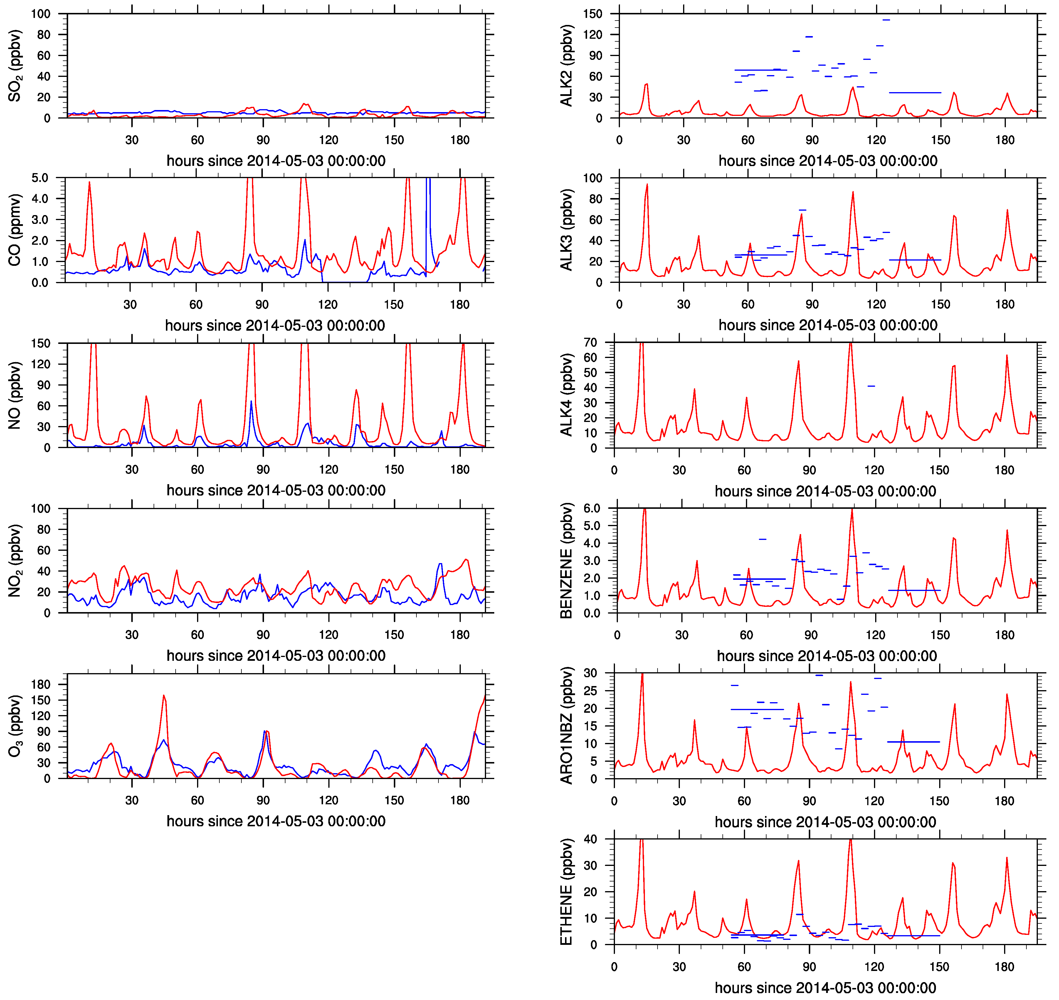
4.3. Comparison with Field Data

4.3.1. Surface Data

The CTM results were compared with the field measurement data. As mentioned above, the mobile emissions were reduced by 40% from the original INEM2008. Figure 8 and Figure 9 show the temporal trends of criteria species and selected SAPRC99 VOC groups at PED station in MCMA and CEN station in GMA during the campaign periods.

Table 3. Fractional bias (FB), normalized mean square error (NMSE), and index of agreement (IA) evaluated at air-monitoring stations during the periods of field campaigns. The evaluation periods were from 3 to 16 of March 2012 in MCMA and from 4 to 11 of May 2014 in GMA. Missing values indicate that field data were missing in more than 25% of the hours during the evaluation periods.

		FB					NMSE					IA
Region	Station (Abbreviation)	O3	CO	NO	NO2	SO2	O3	CO	NO	NO2	SO2	O3	CO	NO	NO2	SO2
MCMA	Chalco (CHO)	−0.54	0.75	1.58	0.32	−0.46	0.50	1.20	27.33	0.74	5.17	0.80	0.48	0.41	0.58	0.24
	Iztacalco (IZT)	−0.12	−0.55	−0.57	−0.21	−0.35	0.25	0.69	2.35	0.21	4.88	0.95	0.75	0.81	0.71	0.38
	Merced (MER)	−0.06	−0.40	−0.47	−0.19	−0.14	0.20	0.60	2.33	0.19	3.43	0.96	0.76	0.81	0.73	0.41
	Pedregal (PED)	−0.21	−0.26	−0.24	−0.11	0.21	0.21	0.26	1.30	0.25	2.19	0.93	0.75	0.87	0.66	0.55
	San Agustin (SAG)	–	–	–	–	–	–	–	–	–	–	–	–	–	–	–
	Santa Ursula (SUR)	−0.18	0.20	−0.29	−0.06	−0.25	0.20	0.27	1.74	0.17	4.12	0.94	0.77	0.84	0.70	0.42
	Tlahuac (TAH)	−0.56	–	0.54	0.21	−0.85	0.50	–	6.39	0.38	7.52	0.79	–	0.60	0.70	0.26
	Tlalnepantla (TLA)	−0.39	−0.53	0.31	0.10	0.35	0.41	0.92	0.87	0.21	3.79	0.88	0.71	0.91	0.75	0.37
	Tultitlan (TLI)	−0.35	−0.37	0.26	−0.08	0.07	0.33	0.56	1.57	0.23	7.33	0.89	0.79	0.88	0.83	0.28
	UAM Iztapalapa (UIZ)	−0.15	0.02	−0.16	−0.22	−0.26	0.19	0.21	0.87	0.21	2.01	0.95	0.86	0.91	0.76	0.55
	Villa de las Flores (VIF)	−0.32	−0.12	0.15	0.08	−0.57	0.19	0.33	2.68	0.37	10.67	0.90	0.84	0.82	0.79	0.21
	Xalostoc (XAL)	−0.26	−0.26	0.68	0.16	−0.06	0.22	0.33	2.13	0.22	2.72	0.92	0.90	0.81	0.79	0.62
GMA	Las Aguilas (AGU)	−0.24	−0.70	−0.58	0.02	0.80	0.61	3.52	11.37	0.81	1.66	0.78	0.18	0.18	0.44	0.50
	Atemajac (ATM)	–	–	–	–	–	–	–	–	–	–	–	–	–	–	–
	Centro (CEN)	0.09	–	−1.32	−0.39	0.51	0.70	–	12.04	0.43	0.90	0.84	–	0.34	0.50	0.18
	Loma Dorada (LDO)	−0.63	−0.40	−0.48	0.00	0.14	1.81	1.42	6.59	0.40	1.53	0.64	0.26	0.39	0.60	0.22
	Las Pintas (LPIN)	–	−0.72	–	–	–	–	2.78	–	–	–	–	0.39	–	–	–
	Miravalle (MIR)	−0.35	−0.64	−0.76	0.01	0.42	1.18	2.69	9.32	0.62	1.05	0.70	0.24	0.37	0.52	0.24
	Oblatos (OBL)	−0.12	−0.70	−0.64	−0.30	–	1.95	4.25	10.50	0.56	–	0.65	0.14	0.18	0.43	–
	Tlaquepaque (TLA)	−0.10	−1.01	−0.96	−0.12	−0.34	0.92	3.92	8.57	0.32	1.80	0.79	0.15	0.31	0.59	0.26
	Vallarta (VAL)	−0.27	–	–	–	–	0.68	–	–	–	–	0.79	–	–	–	–

lists the fractional bias (FB), the normalized mean square error (NMSE), and the index of agreement [29] (IA) for the criteria species at representative air monitoring stations. FB, NMSE, and IA were defined by

$$\begin{array}{ccc}\hfill \mathrm{FB}& =& \frac{2\left(\overline{C_{\mathrm{o}}}-\overline{C_{\mathrm{m}}}\right)}{\overline{C_{\mathrm{o}}}+\overline{C_{\mathrm{m}}}}\hfill \end{array}$$

(3)

$$\begin{array}{ccc}\hfill \mathrm{NMSE}& =& \frac{\overline{{\left(\overline{C_{\mathrm{o}}}-\overline{C_{\mathrm{m}}}\right)}^2}}{\overline{C_{\mathrm{o}}}\overline{C_{\mathrm{m}}}}\hfill \end{array}$$

(4)

$$\begin{array}{ccc}\hfill \mathrm{IA}& =& 1-\frac{\sum {(C_{\mathrm{o}}-C_{\mathrm{m}})}^2}{\sum {\left(|C_{\mathrm{m}}-\overline{C_{\mathrm{o}}}|+|C_{\mathrm{o}}-\overline{C_{\mathrm{o}}}|\right)}^2}\hfill \end{array}$$

(5)

where $C_{\mathrm{o}}$ is the observed value and $C_{\mathrm{m}}$ is the CTM result. According to Chang & Hanna [30], a good performing model should satisfy $|\mathrm{FB}|<0.3$ and $\mathrm{NMSE}<4$. Although there is not an agreed threshold for IA, we regard here $d>0.7$ as a good performance. The results not satisfying these criteria are indicated underlined in Table 3.

Because not all the member compounds in a SAPRC99 VOC species were measured during the campaign periods, only those SAPRC99 VOC species were selected for which the measured compounds occupied more than 70% of the total members on the basis of the speciated amount in INEM2008.

In MCMA, the CTM results and field data agree fairly well for both criteria and VOC species. The poor agreement for SO₂ is due to the large emissions from fixed sources that occur irregularly in the northern industrial area. The poor performance for CO and NO at Chalco (CHO) in MCMA should be commented. For both species, the CTM was severe underestimation, especially in the morning rush hours. Chalco is located in the south-eastern part of the Mexico City basin (see Figure 1b) where the density of the road network is much less than in the central part of the Federal District. However, about 450 m to the east of the CHO station, there is a federal road that connects the Mexico City basin and the southern municipalities through the narrow gap between the rim mountains. In the CTM grid, the emission from this road is uniformly distributed in the 3 km × 3 km area, but in reality, the CHO station is likely to receive the relatively dense plume from the traffic emission that was probably underestimated by our crude method of allocating 4 times more emissions to federal and state roads than to other roads.

With the original INEM2008 without modification of the road mobile emissions, CTM results for CO, NO_x, ALK4, BENZENE, and ARO1NBZ became considerably larger than the field data whereas that for ALK2 was a little overestimation and that for ALK3 agreed well with the field data. Because most of ALK2 and ALK3 are LPG compounds (propane and butane) that derive from area sources and because these species due to the small OH-reactivity are little affected by the model errors, INEM2008 was considered correct for the area sources. Most of the overestimated species, particularly the slow reacting CO that is relatively insensitive to errors in the chemical modeling, derived from mobile sources. In INEM2008, problems with mobile sources are pointed out by many researchers at Mexican environment authorities (personal communications): (1) the number of vehicles used in INEM2008 is based on registration, but the actual number is likely to be much smaller because there is no obligation for car owners to cancel the previous registration record when they sell their vehicles to someone else outside the initial registration states; (2) the activity (mileage) may be subject to large uncertainties because of the primitive survey methods such as questionnaire at gas stations or recording of travel meters at the time of exhaust-gas inspection (conducted only in the Federal District); and (3) the emission factor used in calculating the emission rate may have large uncertainty because no extensive exhaust-gas examination by chassis dynamometer or no road-tunnel measurement has been conducted in Mexico.

Therefore, it was considered adequate to adjust the road mobile emissions. For simplicity, all the emission species from road mobile sources were multiplied by a factor. By trial and error, a factor 0.6 turned out to produce a balanced agreement between the CTM results and the field data in MCMA. As a tentative adjustment, the same factor was applied to GMA.

In GMA, the CTM results tended to underestimate many VOC species: ALK2, ALK3, BENZENE, and ARO1NBZ. It was, however, suspected that the area-source emissions were underestimated because the CEN station is located in the downtown area where commercial activity is highly concentrated, a situation the present emission distribution method could not handle correctly. In contrast, the PED station in MCMA is located in a residential area separated from concentrated emissions.

In GMA, CO and NO concentrations were overestimated by CTM. Note that, because the data of CO was missing at the CEN station during the field campaign, Figure 9 shows the trend at the OBL station northeast of the CEN station (see Figure 1a). The overestimation occurred mainly in the morning rush hours. Because both CO and NO derive primarily from road mobile sources, further reduction of emissions from road mobile sources seemed necessary. Because many VOC species were underestimated by CTM, this suggests different modification factors for different species (disregarding the peculiar situation around the CEN station). Although better agreement could be obtained by modifying emission rates in a sophisticated manner, we decided not to do so because the quality of regular monitoring in GMA is not as high as that in MCMA according to the audit results by INECC (personal communication). As discussed in Section 4.4, the current level of the agreement obtained by CTM using INEM2008 modified by multiplying the road mobile emissions by 0.6 is sufficient to deduce the O₃ formation regime in GMA.

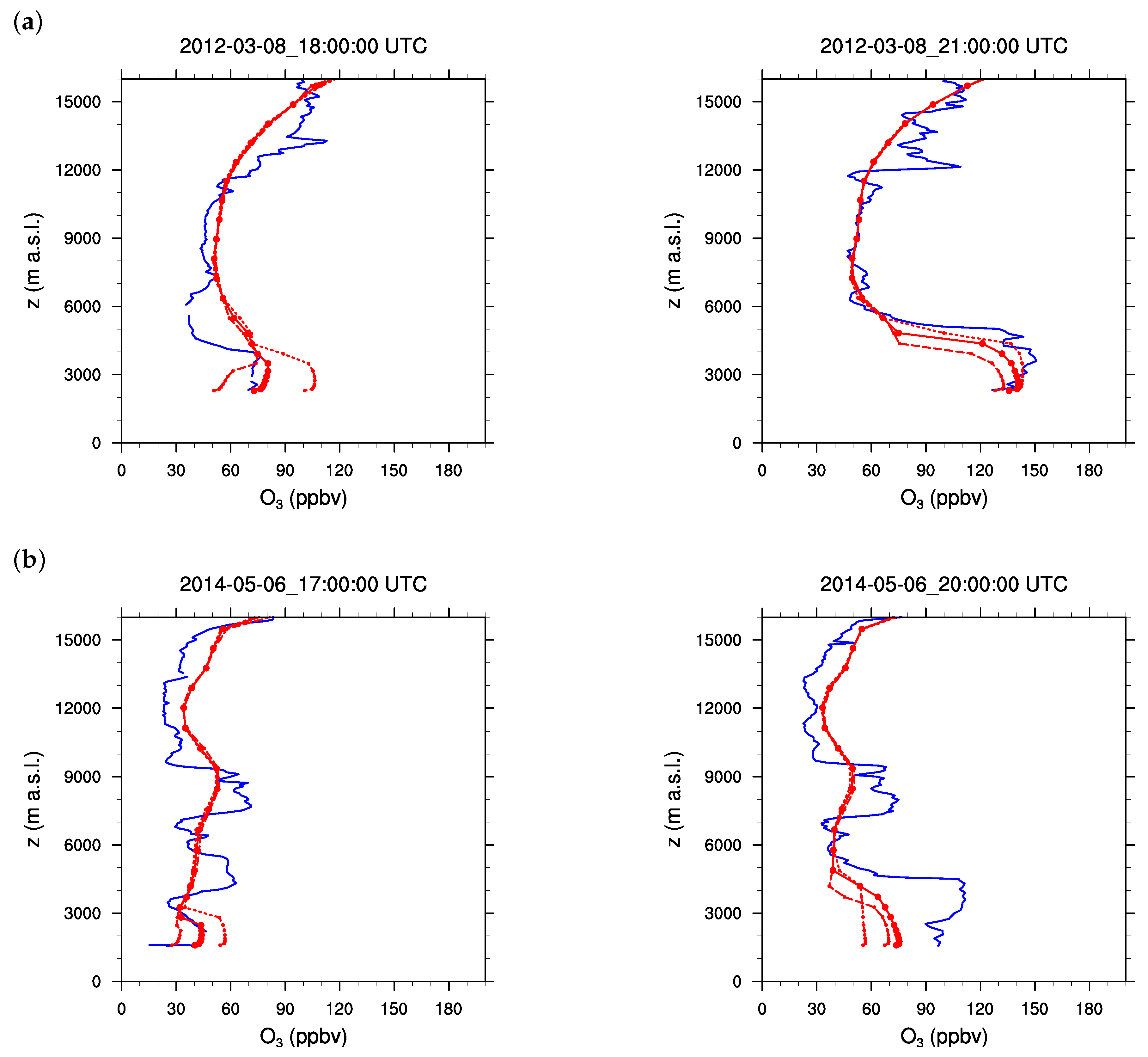
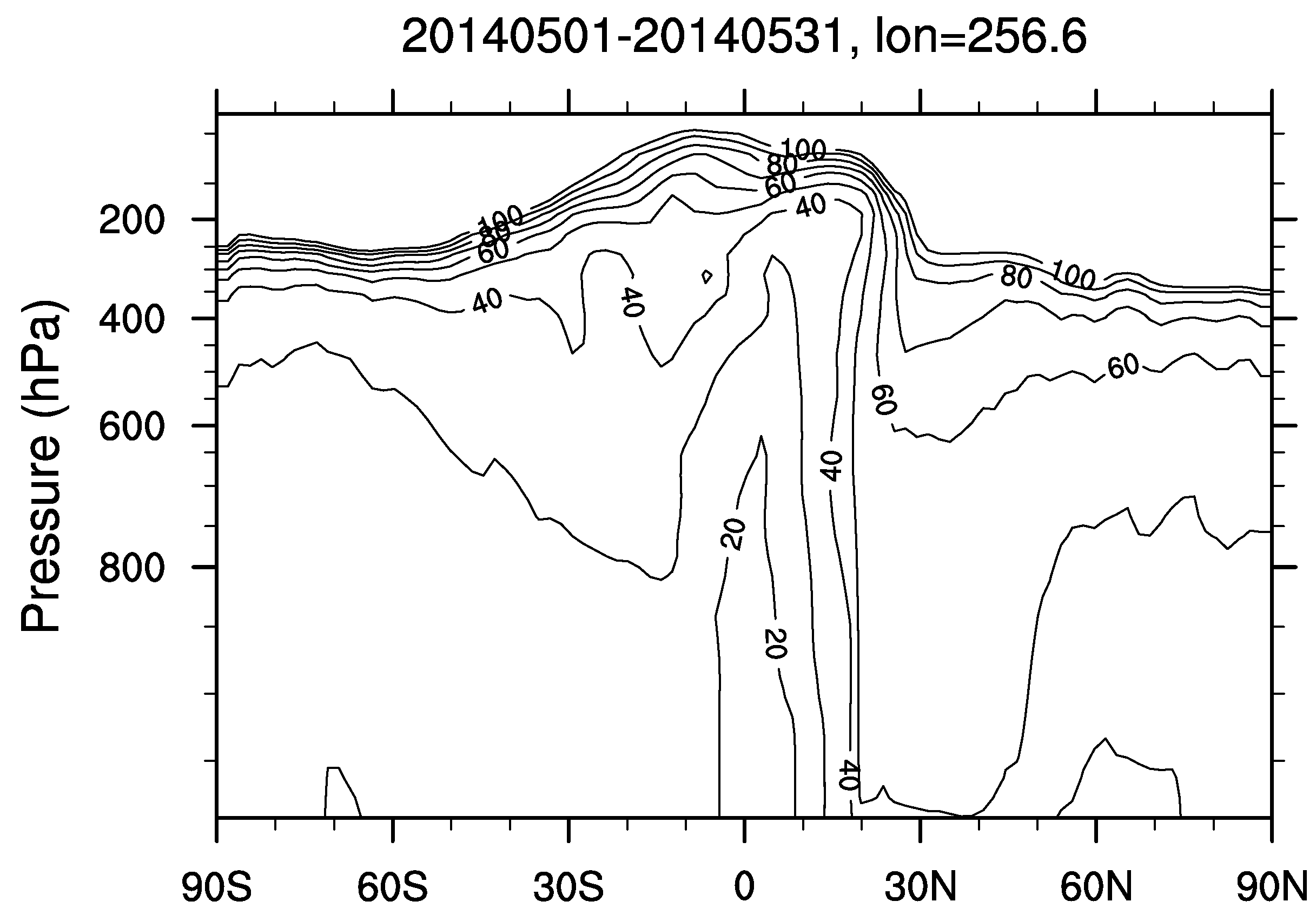
4.3.2. Vertical Profiles of O₃

Because tropospheric O₃ is produced mainly by photochemical reactions, its concentration usually maximizes in the afternoon, when the emissions of precursor substances are high and the ultraviolet radiation is also high. At the same time, natural convection brings O₃ and precursor substances to higher altitudes where photochemistry is more intense (at diluted concentrations) due to the higher ultraviolet radiation. Hence, it is important to validate CTM simulations against vertical profiling data of O₃ concentration.

Figure 10 shows simulated and observed vertical profiles of O₃ concentration in the morning and afternoon on a day when the weather was fine with visually determined cloud coverage less than 0.9, and the O₃ concentration at the ozonesonde observation site was highest among the observation days. The CTM profiles represent averages in 9 grid cells around the observation site although almost the same profiles were obtained using only the cell that included the observation site. The CTM results drawn by solid line are the instantaneous values at 30 min after the ozonesonde launching time when the observation balloons reached about 9 km above the ground. The CTM results of one hour before and after are also drawn by long-dashed and short-dashed line, respectively. A notable feature in MCMA and GMA is the relatively high convective mixing layer of about 3 km in the afternoon. In MCMA, the CTM results agreed well with the observations both in the morning and afternoon.

In GMA, CTM underestimated the concentration in the convective mixing layer considerably. One reason for the poor performance is the temporally narrow peak of O₃ concentration on this day (compare the peak around 90 h in the bottom-left panel in Figure 9 with other peaks). On this day, the high-O₃ urban plume was transported toward northeast relatively quickly and the residence time over the GMA core was short. Although the peak hour and the magnitude were reproduced well at the CEN station (Figure 9), the same level of agreement could not be achieved everywhere in GMA. Actually, the vertical profile of the CTM profile of O₃ concentration at the CEN station at 20:00 UTC on 6 May 2014 agreed well with the ozonesonde observation at the meteorological observatory except for the large bulge around 3500 m a.s.l. It should be noted that the observation balloon had traveled only 120 m to the north of the launching site by the time it reached 3 km a.s.l.

In addition to the overall underestimation, an important difference is a bulge from 3 to 4.5 km a.s.l. Similar upper-air peaks were observed around 8.5 km a.s.l. at the time of Figure 10 and at various heights at other occasions during the GMA campaign in May 2014. The origin of these peaks is considered to be the stratosphere-troposphere exchange that becomes active in spring in the northern hemisphere. Indeed, the air was dry, and a stable stratification existed around the peaks of O₃ concentration, characteristics of airmass originating from the stratosphere. Figure 11 shows the meridional-vertical section of O₃ concentration averaged through May 2014 at the Guadalajara longitude calculated by the MOZART-4/GEOS-5 global chemical modeling system [31]. In 2014, it was only in April and May when the 50 ppb contour was on or south of 20°N in the lower troposphere. Although backward trajectories from the heights of O₃ maxima calculated by HYSPLIT [32] were found to originate from the upper troposphere (≳10 km a.s.l.) above the Pacific Ocean, the MOZART-4/GEOS-5 results that were adopted as the chemical boundary condition in the outermost nest (d01) in our CTM simulation did not always reproduce the observed upper-air maxima of O₃ concentration correctly. The blunt peak of the CTM result around 9 km a.s.l. in Figure 10 was induced by a similar peak at about the same height in the MOZART-4/GEOS-5 simulation, but the observed peak around 3.5 km a.s.l. could not be reproduced with our CTM configuration.

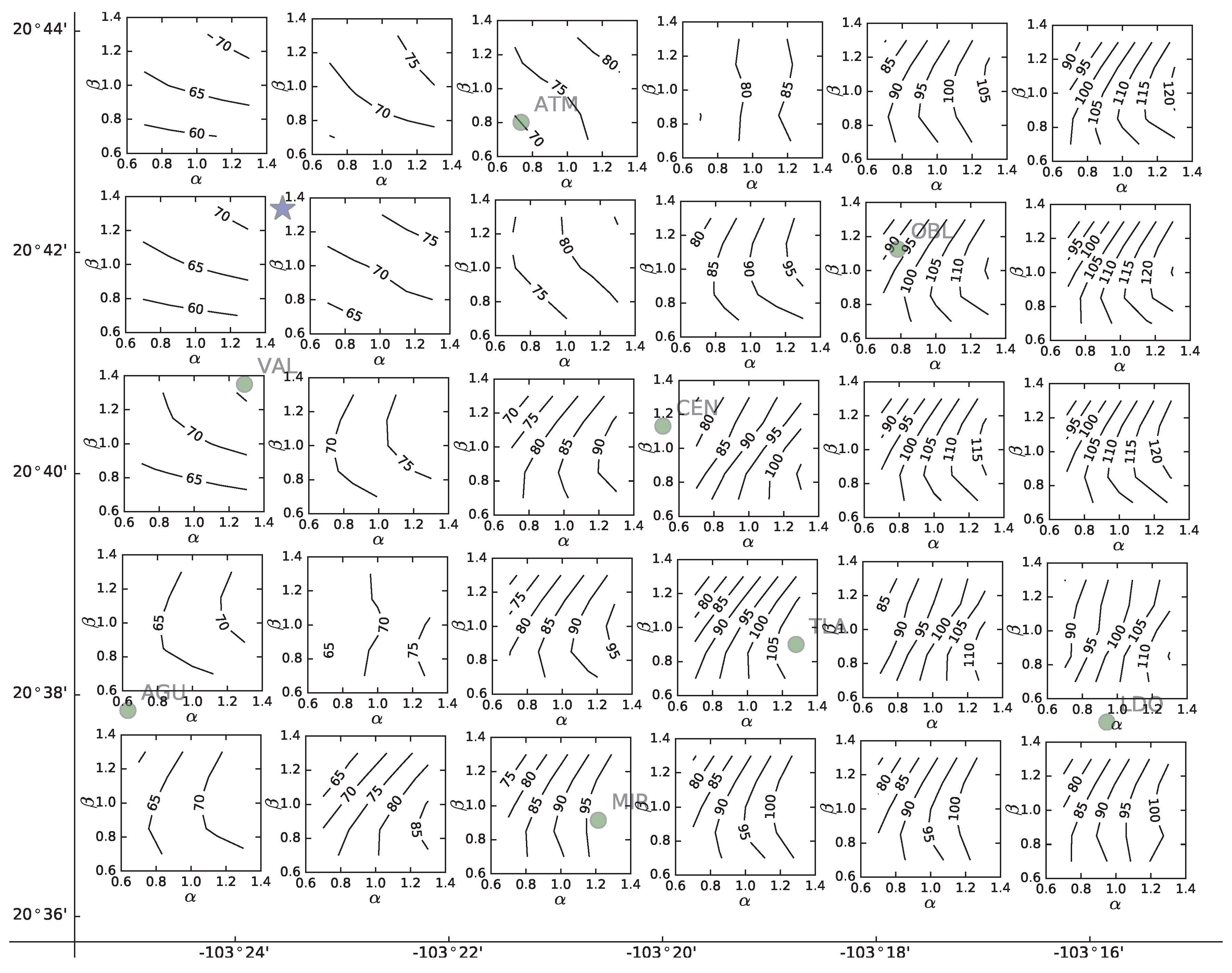
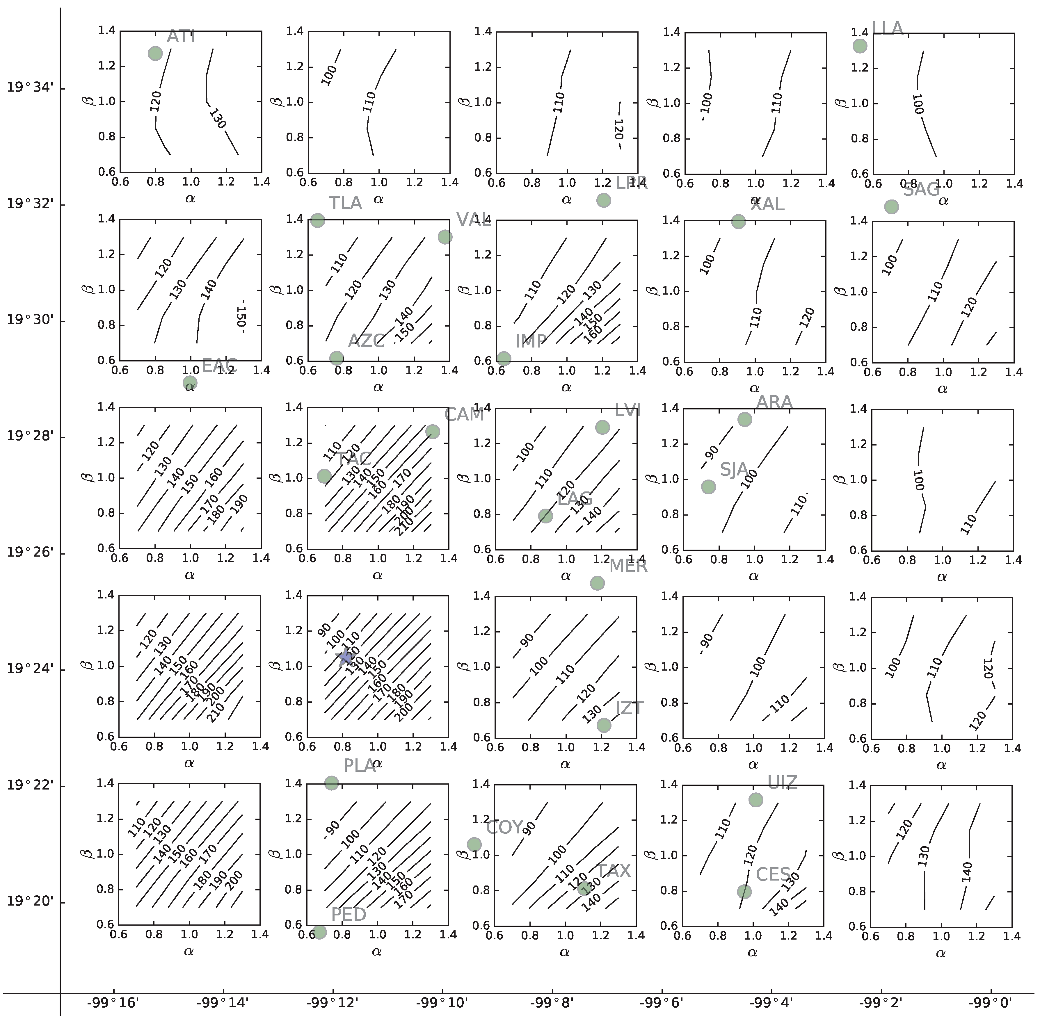
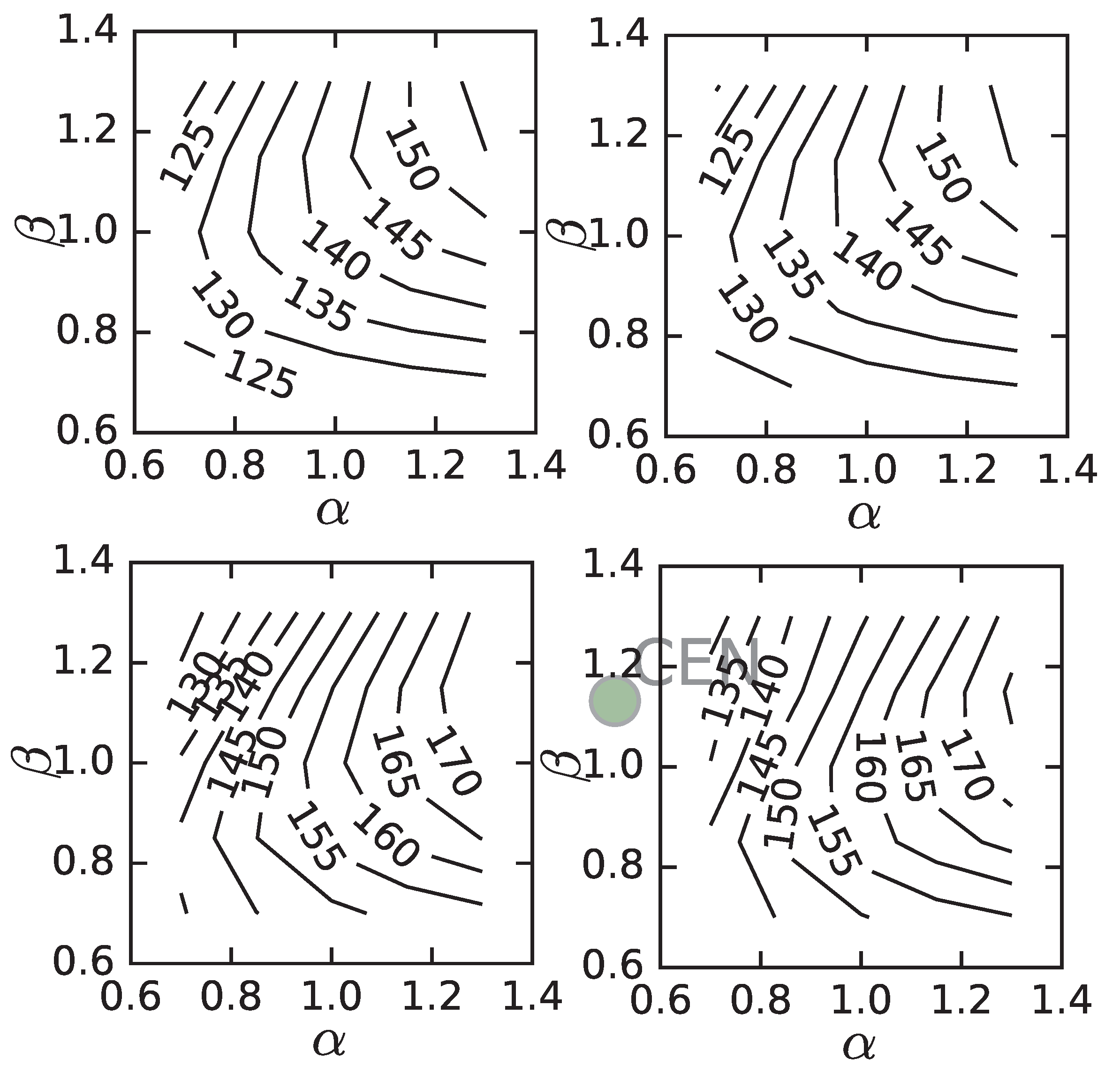
4.4. Ozone Formation Regime

The O₃ formation regime was examined by conducting CTM simulations with modified NO_x and VOC emissions. The modifications were done by multiplying a factor ranging in 0.7, 0.85, 1.0, 1.15, and 1.3 to NO_x or VOC uniformly in space and time for the anthropogenic emissions in the inner-most domain d03 (see Table 2). The maximum variation magnitude of 30% is “comparable to the scale of emission reductions that policy-makers commonly consider” [33]. The test cases are denoted by the multiplication factors α and β on VOC and NO_x, respectively. The daily maximum $C_{\max }$ of hourly averaged O₃ concentration was evaluated for each test case $(\alpha ,\beta )$. Figure 12 and Figure 13 shows the contours of $C_{\max }$ in $(\alpha ,\beta )$ coordinate space at the simulation grid cells in the urban cores of MCMA and GMA on 8 March 2012 and 6 May 2014, respectively. The aim of the map presentation is to show the general characteristics among the variabilities due to various forms of uncertainties in the simulation. The background of Figure 12, Figure 13 and Figure 14 is a geographical map with the meteorological observatory and the air-quality monitoring stations indicated at their geographical coordinates. The centers of the plot panels coincide with the cell centers of the CTM simulation grid.

In many of the MCMA grid cells, $C_{\max }$ increases with increasing α and decreasing β, i.e., the O₃ formation regime is VOC-sensitive. Similar $C_{\max }$-contours were obtained on other days during the campaign period. The result agrees with the previous work [2]. For the base case $\alpha =\beta =1$, the daily maximum occurred most frequently in 14–15 LST. The peak hour became earlier for larger $\alpha /\beta$, consistent with the large production rate of O₃ when $\alpha /\beta$ is large (e.g., [34]).

In many of the GMA grid cells, $C_{\max }$ increases with α but the dependence on β is much weaker than in MCMA, i.e., a ridge of $C_{\max }$ contour can be discerned in the tested range of $(\alpha ,\beta )$ space. Similar $C_{\max }$-contours were obtained on other days during the campaign period. For the base case $\alpha =\beta =1$, the daily maximum occurred most frequently in 13-14 LST, an hour earlier than in MCMA. The earlier peak hour is consistent with the higher VOC/NO_x emission ratio in GMA than in MCMA (Figure 6b). (Note that VOC in Figure 6b indicates the OLT-equivalent molar amount whereas VOC in this section indicates the total mass irrespective of the OH-reactivity.) As in MCMA, the peak hour became earlier for larger $\alpha /\beta$. On 4 May 2014 (Sunday) when a higher O₃ concentration was observed with temporally broader maxima than on 6 May 2014, a ridge of $C_{\max }$ was clearly seen at a majority of the grid cells. Note that the high O₃ concentration is attributable to the weekend effect [35] due to the reduced emissions on Sunday. Figure 14 illustrates the result at the four grid cells around the CEN station.

In GMA, isoprene originating from the biogenic sources in the area near the Pacific ocean was observed to be transported eastward in the simulation result for the d02 domain. The peak values of the simulated isoprene concentration in GMA was about 5 ppb, rather high considering the large OH-reactivity of isoprene. However, because the peak hours were usually around midnight, the effect on ozone formation was considered small.

In the previous section, the comparison between CTM and surface observation implied that NO_x might be overestimated and VOC might be underestimated in the adopted emissions grid. If the implication were true, the location in $(\alpha ,\beta )$ space would be shifted further away from the VOC-sensitive regime toward the NO_x-sensitive regime. It can, therefore, be estimated roughly that the O₃ formation in the current GMA lies in the intermediate region between VOC-sensitive and NO_x-sensitive regimes. The difference between MCMA and GMA is consistent with the relatively large VOC/NO_x ratio of emissions in GMA compared to that in MCMA (Figure 6b).

5. Conclusions

CTM simulations were conducted to gain a better understanding of the present condition of photochemical O₃ production in GMA where a gradual increase of the ground-level concentration of O₃ has been observed over the past decade. As input to the CTM simulations, emissions grids were constructed based on the national inventory INEM2008 that was modified by reducing the road mobile emissions by 40%. The annual emissions allocated to municipalities were distributed in space and time using various geographical and survey data. Analysis of the gridded emissions revealed that the emission ratio VOC/NO_x in the urban area is greater in GMA than in MCMA due mainly to the older unregulated vehicle fleet in GMA. The CTM results were found appropriate by comparison with routine ground-level monitoring data of criteria pollutants and field campaign data of VOC analysis and ozonesonde vertical profiling. By numerical experiments in which the overall emission rates of NO_x and VOC were varied, the O₃ formation in GMA was found to be in the intermediate phase between VOC-sensitive and NO_x-sensitive regimes whereas that in MCMA was confirmed to be in the VOC-sensitive regime as in previous research [2]. Although the comparison between the CTM results and the observation data indicated that further adjustment of the emissions inventory might be necessary, the O₃ production regime in GMA was not likely to shift substantially toward distinct VOC-sensitive or NO_x-sensitive regime.

In this study, validation of CTM simulations by ozonesonde data was not very satisfactory in GMA. Because high O₃ concentration is usually observed in May and June in GMA, we planned our international field campaign in May, avoiding June with frequent rainy days. In May, however, we realized later that stratosphere-troposphere exchange is active and upper-air intrusion is frequent that adds a variable to the comparison between CTM and observation. To secure useful validation data of vertical profiles of O₃ concentration, one may have to launch ozonesonde on a regular basis.

In GMA, VOC observation downwind, i.e., east, of the downtown area may be necessary to evaluate the photochemical condition in a robust manner. In MCMA, the PED station located in a residential area downwind of the city center provided ideal data for CTM validation. Note that observation in the downtown area should be conducted as well for the purpose of environmental assessment because some species such as benzene are toxic by themselves although the O₃-producing potential is low.

The GMA atmosphere is likely to shift toward the VOC-sensitive regime if stricter automobile exhaust regulation is implemented, which tends to decrease VOC more rapidly than NO_x as happened in MCMA and other metropolitan areas [2,4,5,36]. In the VOC-sensitive regime, increase of NO_x would reduce O₃ but would result in increases of NO₂ that is associated with respiratory diseases and also result in increases of nitrate particles that could reduce visibility. Therefore, mitigation strategy has to be planned carefully with a long-term vision based on sound scientific evidence. This study, providing a starting point, needs to be complemented by further research based on more reliable emissions inventory, longer-term surface observation data including VOC and odd nitrogen at multiple sites, and more vertical profiling of O₃.

References

1. Benítez-García, S.E.; Kanda, I.; Wakamatsu, S.; Okazaki, Y.; Kawano, M. Analysis of criteria air pollutant trends in three Mexican metropolitan areas. Atmosphere 2014, 5, 806–829. [Google Scholar] [CrossRef]
2. Molina, L.T.; Madronich, J.S.; Gaffney, J.S.; Apel, E.; de Foy, B.; Fast, J.; Ferrare, R.; Herndon, S.; Jimenez, J.L.; Lamb, B.; et al. An overview of the MILAGRO 2006 Campaign: Mexico City emissions and their transport and transformation. Atmos. Chem. Phys. 2010, 10, 8697–8760. [Google Scholar] [CrossRef] [Green Version]
3. Seinfeld, J.H.; Pandis, S.N. Atmospheric Chemistry and Physics: From Air Pollution to Climate Change; John Wiley & Sons: Hoboken, NJ, USA, 2006. [Google Scholar]
4. Sillman, S.; Vautard, R.; Menut, L.; Kley, D. O3-NOx-VOC sensitivity and NOx-VOC indicators in Paris: Results from models and Atmospheric Pollution Over the Paris Area (ESQUIF) measurements. J. Geophys. Res. 2003, 108, 8563. [Google Scholar] [CrossRef]
5. Kleinman, L.I.; Daum, P.H.; Lee, Y.-N.; Nunnermacker, L.J.; Springston, S.R.; Weinstein-Lloyd, J.; Rudolph, J. A comparative study of ozone production in five U.S. metropolitan areas. J. Geophys. Res. 2005, 110, D02301. [Google Scholar] [CrossRef]
6. Sillman, S.; Al-Wali, K.I.; Marsik, F.J.; Nowacki, P.; Samson, P.J.; Rodgers, M.O.; Garland, L.J.; Martinez, J.E.; Stoneking, C.; Imhoff, R.; et al. Photochemistry of ozone formation in Atlanta, GA—Models and measurements. Atmos. Environ. 1995, 29, 3055–3066. [Google Scholar] [CrossRef]
7. Ramírez-Sánchez, H.U.; Andrade-García, M.D.; Bejaran, R.; García Guadalupe, M.E.; Wallo Vázquez, A.; Pompa Toledano, A.C.; de la Torre Villaseñor, O. The spatial-temporal distribution of the atmospheric polluting agents during the period 2000–2005 in the urban area of Guadalajara, Jalisco, Mexico. J. Hazard. Mater. 2009, 165, 1128–1141. [Google Scholar] [CrossRef] [PubMed]
8. Jaimes-Lopez, J.L.; Sandoval-Fernandez, J.; Gonzalez-Ortiz, E.; Vazquez-Garcia, M.; Gonzalez-Macias, U.; Zambrano-Garcia, A. Effect of liquefied petroleum gas on ozone formation in Guadalajara and Mexico City. J. Air Waste Manag. Assoc. 2005, 55, 841–846. [Google Scholar] [CrossRef] [PubMed]
9. Mendoza, A.; Garcia, M.R. Application of a second-generation air quality model to the Guadalajara metropolitan area, Mexico. Rev. Int. Contam. Ambient. 2009, 25, 73–85. [Google Scholar]
10. Harley, H.A.; Russel, A.G.; McRae, G.J.; Cass, G.R.; Seifeld, J.H. Photochemical modeling of the southern California air quality study. Environ. Sci. Technol. 1993, 27, 378–388. [Google Scholar] [CrossRef]
11. Mendoza, A.; Garcia, M.R. Inverse modeling applied to the analysis of emission inventory of the metropolitan area of Guadalajara, Mexico. Rev. Int. Contam. Ambient. 2011, 27, 199–214. [Google Scholar]
12. Escarela, G. Extreme value modeling for the analysis and prediction of time series of extreme tropospheric ozone levels: A case study. J. Air Waste Manag. Assoc. 2012, 62, 651–661. [Google Scholar] [CrossRef] [PubMed]
13. García, I.; Marbán, A.; Tenorio, Y.M.; Rodriguez, J.G. Ozone concentration forecast in Guadalajara-Mexico using artificial neuronal networks. Inf. Tecnol. 2008, 19, 89–96. [Google Scholar]
14. Byun, D.; Schere, K.L. Review of the governing equations, computational algorithms, and other components of the Models-3 Community Multiscale Air Quality (CMAQ) modeling system. Appl. Mech. Rev. 2006, 59, 51–77. [Google Scholar] [CrossRef]
15. Whiteman, C.D.; Zhong, S.; Bian, X.; Fast, J.D.; Doran, J.C. Boundary layer evolution and regional-scale diurnal circulations over the Mexico Basin and Mexican plateau. J. Geophys. Res. 2000, 105, 10081–10102. [Google Scholar] [CrossRef]
16. Kanda, I.; Basaldud, R.; Horikoshi, N.; Okazaki, Y.; Benítez-Garcia, S.E.; Ortínez, A.; Ramos Benítez, V.R.; Cárdenas, B.; Wakamatsu, S. Interference of sulphur dioxide on balloon-borne electrochemical concentration cell ozone sensors over the Mexico City metropolitan area. Asian J. Atmos. Environ. 2014, 8, 162–174. [Google Scholar] [CrossRef]
17. Benítez-García, S.E.; Kanda, I.; Wakamatsu, S.; Okazaki, Y.; Kawano, M. Investigation of vertical profiles of meteorological parameters and ozone concentration in the Mexico City metropolitan area. Asian J. Atmos. Environ. 2015, 9, 114–127. [Google Scholar]
18. Garzón, J.P.; Huertas, J.I.; Magaña, M.; Huertas, M.E.; Cárdenas, B.; Watanabe, T.; Maeda, T.; Wakamatsu, S. Volatile organic compounds in the atmosphere of Mexico City. Atmos. Environ. 2015, 119, 415–429. [Google Scholar] [CrossRef]
19. Jaimes-Palomera, M.; Retama, A.; Elias-Castro, G.; Neria-Hernández, A.; Rivera-Hernández, O.; Velasco, E. Non-methane hydrocarbons in the atmosphere of Mexico City: Results of the 2012 ozone-season campaign. Atmos. Environ. 2016, 132, 258–275. [Google Scholar] [CrossRef]
20. Komhyr, W.D.; Barnes, R.A.; Brothers, G.B.; Lathrop, J.A.; Opperman, D.P. Electrochemical concentration cell ozonesonde performance evaluation during STOIC 1989. J. Geophys. Res. 1995, 100, 9231–9244. [Google Scholar] [CrossRef]
21. Instituto Nacional de Estadística y Geografía (INEGI). Available online: http://www.inegi.org.mx/geo/contenidos/recnat/usosuelo/ (accessed on 1 February 2016).
22. OpenStreetMap. Available online: https://www.openstreetmap.org/ (accessed on 1 February 2016).
23. Statistics Bureau, Japan Ministry of Internal Affairs and Communications. Basic Survey of Social life. 2006; (In Japanese). Available online: http://www.stat.go.jp/data/shakai/2006/gaiyou.htm (accessed on 1 February 2016). [Google Scholar]
24. U.S. Environmental Protection Agency. Available online: http://www3.epa.gov/ttn/chief/emch/speciation/ (accessed on 1 February 2016).
25. Carter, W.P.L. Development of an Improved Chemical Speciation Database for Processing Emissions of Volatile Organic Compounds for Air Quality Models. Available online: http://www.engr.ucr.edu/~carter/emitdb/ (accessed on 1 February 2016).
26. Morikawa, T. Source speciation profiles VOC, PM, and NOx for PM2.5 regional air-quality simulations. In Japan Auto-Oil Program Technical Report; Japn Auto-Oil Program: Tokyo, Japan, 2012; JPEC-2011AQ-02-08. [Google Scholar]
27. Skamarock, W.C.; Klemp, J.B.; Dudhia, J.; Gill, D.O.; Barker, D.M.; Duda, M.G.; Huang, X.-Y.; Wang, W.; Powers, J.G. A Description of the Advanced Research WRF; NCAR/TN-475+STR; NCAR UCAR OpenSky. Available online: http://nldr.library.ucar.edu/repository/collections/TECH-NOTE-000-000-000-855 (accessed on 15 July 2016).
28. Guenther, A.B.; Jiang, X.; Heald, C.L.; Sakulyanontvittaya, T.; Duhl, T.; Emmons, L.K.; Wang, X. The Model of Emissions of Gases and Aerosols from Nature version 2.1 (MEGAN2.1): An extended and updated framework for modeling biogenic emissions. Geosci. Model Dev. 2012, 5, 1471–1492. [Google Scholar] [CrossRef] [Green Version]
29. Willmott, C.J. On the validation of models. Phys. Geogr. 1981, 2, 184–194. [Google Scholar]
30. Chang, J.C.; Hanna, S.R. Air quality model performance evaluation. Meteorol. Atmos. Phys. 2004, 87, 167–196. [Google Scholar] [CrossRef]
31. National Center for Atmospheric Research, Atmospheric Chemistry Observations and Modeling. Available online: http://www.acom.ucar.edu/gctm/mozart/subset.shtml (accessed on 1 February 2016).
32. HYSPLIT - Hybrid Single Particle Lagrangian Integrated Trajectory Model, Air Resources Laboratory. Available online: http://ready.arl.noaa.gov/HYSPLIT.php (accessed on 1 February 2016).
33. Derwent, R.; Beevers, S.; Chemel, C.; Cooke, D.; Francis, X.; Fraser, A.; Heal, M.R.; Kitwiroon, N.; Lingard, J.; Redington, A.; et al. Analysis of UK and European NOx and VOC emission scenarios in the Defra model intercomparison exercise. Atmos. Environ. 2014, 94, 249–257. [Google Scholar] [CrossRef] [Green Version]
34. Kleinman, L.I.; Daum, P.H.; Imre, D.; Lee, Y.-N.; Nunnermacker, L.J.; Springston, S.R.; Weinstein-Lloyd, J.; Rudolph, J. Ozone production rate and hydrocarbon reactivity in 5 urban areas: A cause of high ozone concentration in Houston. Geophys. Res. Lett. 2002, 29, 1467. [Google Scholar] [CrossRef]
35. California Environmental Protection Agency. Available online: http://www.arb.ca.gov/research/weekendeffect/weekendeffect.htm (accessed on 3 July 2016).
36. Song, J.; Lei, W.; Bei, N.; Zavala, M.; de Foy, B.; Volkamer, R.; Cardenas, B.; Zheng, J.; Zhang, R.; Molina, L.T. Ozone response to emission changes: A modeling study during the MCMA-2006/MILAGRO Campaign. Atmos. Chem. Phys. 2010, 10, 3827–3846. [Google Scholar] [CrossRef] [Green Version]
37. Molina, L.T.; Molina, M.J. Air Quality in the Mexico Megacity: An Integrated Assessment; Springer Science+Business Media: Dordrecht, The Netherlands, 2002. [Google Scholar]
Figure 1. Central parts of GMA (a) and MCMA (b). Gray shade indicates the urban landuse area. Circles indicate the air-monitoring stations. Filled circles are selected stations listed in Table 3. Stars indicate the locations of the meteorological observatories where ozonesonde was launched. Elevation contours are drawn at 200 m intervals.
Atmosphere 07 00091 g001
Figure 2. Activity coefficients T ^ s ( d , h ) of “human” and “household” activity derived from a Japanese survey [23]. T ^ s ( d , h ) does not depend on d.
Atmosphere 07 00091 g002
Figure 3. Activity coefficients T ^ s ( d , h ) of passenger cars (A) and trucks (C) defined as average traffic flow rates in the traffic census conducted in 2003 in MCMA. The day index d ranges from 0 (Monday) to 6 (Sunday), and the hour index h ranges from 0 to 23. Note that letter B is assigned to public transportation, which is not plotted because of the large fluctuations due to the small traffic volume, in the original traffic census database.
Atmosphere 07 00091 g003
Figure 4. Gridded distribution of time-averaged emission intensities of NO and VOC (equivalent to OLT in RADM2 in terms of OH-reactivity) summed over the vertical layers. SMN (an acronym for the Spanish name Servicio Meteorológico Nacional) denotes meteorological observatory, and AQ station denotes air-quality monitoring station. Elevation contours are drawn at 500 m intervals beginning with 500 m.
Atmosphere 07 00091 g004
Figure 5. Proportions of fixed, area, and mobile sources in the anthropogenic emissions of NOx and VOC (equivalent to OLT in RADM2 in terms of OH-reactivity). Only emissions in urban grid cells were taken into account. The radius of a pie chart is proportional to the total emission rate relative to that in MCMA. (a-1) MCMA, NOx, (a-2) MCMA, VOC, (b-1) GMA, NOx, (b-2) GMA, VOC.
Atmosphere 07 00091 g005
Figure 6. Emissions of NOx and VOC (equivalent to OLT in RADM2 in terms of OH-reactivity) in the urban grid cells of MCMA and GMA. (a) Emission intensity per area; (b) VOC/NOx ratio.
Atmosphere 07 00091 g006
Figure 7. WRF simulation domains for GMA (a) and MCMA (b). The panel frame corresponds to the outermost domain d01. The circle indicates the meteorological observatory where ozonesonde observation was conducted.
Atmosphere 07 00091 g007
Figure 8. Comparison between field data (blue) and CTM simulations (red) at Pedregal (PED) station in MCMA.
Atmosphere 07 00091 g008
Figure 9. Comparison between field data (blue) and CTM simulations (red) in GMA. The location is the Centro (CEN) station except for CO that was evaluated at the Oblatos (OBL) station because the data at the Centro station was missing.
Atmosphere 07 00091 g009
Figure 10. Comparison of vertical profiles of O3 concentration between ozonesonde observations (blue) and CTM simulations (red). (a) MCMA; (b) GMA. Solid line with large circle markers indicates the CTM result at the target time indicated above each panel while long-dashed and short-dashed lines with small circle markers indicate the CTM results of one hour before and after the target time, respectively. The CTM results represent averages in 9 grid cells around the observation site. The local standard time is the indicated UTC minus 6 h. Note that the daylight-saving time was in effect during the GMA campaign.
Atmosphere 07 00091 g010
Figure 11. Meridional-vertical section of O3 concentration (ppb) averaged through May 2014 at the Guadalajara longitude calculated by the MOZART-4/GEOS-5 global chemical modeling system [31].
Atmosphere 07 00091 g011
Figure 12. Contour plots of daily maximum O3 concentration in ( α , β ) space on 8 March 2012 in MCMA, where α and β denote the multiplication factors on the emission rates of VOC and NOx, respectively. The plot panels are shown at every other grid points, i.e., at 6 km spacing. The star marker indicates the meteorological observatory where ozonesonde was launched. The circles indicate the air monitoring stations denoted by abbreviations, some of which are listed in Table 3.
Atmosphere 07 00091 g012
Figure 13. Contour plots of daily maximum O3 concentration in ( α , β ) space on 6 May 2014 in GMA, where α and β denote the multiplication factors on the emission rates of VOC and NOx, respectively. The plot panels are shown at all the grid points, i.e., at 3 km spacing. The star marker indicates the meteorological observatory where ozonesonde was launched. The circles indicate the air monitoring stations denoted by abbreviations, some of which are listed in Table 3.
Atmosphere 07 00091 g013
Figure 14. Contour plots of daily maximum O3 concentration on ( α , β ) space on 4 May 2014 in GMA, where α and β denote the multiplication factor on the emission rates of VOC and NOx, respectively. Only the results in the four grid cells near the Centro (CEN) station are shown.
Atmosphere 07 00091 g014