Feasibility Study of Multi-Wavelength Differential Absorption LIDAR for CO₂ Monitoring

Abstract

To obtain a better understanding of carbon cycle and accurate climate prediction models, highly accurate and temporal resolution observation of atmospheric CO₂ is necessary. Differential absorption LIDAR (DIAL) remote sensing is a promising technology to detect atmospheric CO₂. However, the traditional DIAL system is the dual-wavelength DIAL (DW-DIAL), which has strict requirements for wavelength accuracy and stability. Moreover, for on-line and off-line wavelengths, the system’s optical efficiency and the change of atmospheric parameters are assumed to be the same in the DW-DIAL system. This assumption inevitably produces measurement errors, especially under rapid aerosol changes. In this study, a multi-wavelength DIAL (MW-DIAL) is proposed to map atmospheric CO₂ concentration. The MW-DIAL conducts inversion with one on-line and multiple off-line wavelengths. Multiple concentrations of CO₂ are then obtained through difference processing between the single on-line and each of the off-line wavelengths. In addition, the least square method is adopted to optimize inversion results. Consequently, the inversion concentration of CO₂ in the MW-DIAL system is found to be the weighted average of the multiple concentrations. Simulation analysis and laboratory experiments were conducted to evaluate the inversion precision of MW-DIAL. For comparison, traditional DW-DIAL simulations were also conducted. Simulation analysis demonstrated that, given the drifting wavelengths of the laser, the detection accuracy of CO₂ when using MW-DIAL is higher than that when using DW-DIAL, especially when the drift is large. A laboratory experiment was also performed to verify the simulation analysis.

1. Introduction

Global warming is now considered indisputable, a fact that has been further confirmed by the fifth working report of the International Panel of Climate Change (IPCC). Greenhouse gas emissions and other human-driven factors have been the main causes of global warming since the mid-20th century [1,2,3]. The concentration of atmospheric CO₂, which is one of the most important greenhouse gases, has increased by more than 100 parts per million (ppm) from approximately 280 to 400 ppm since the Industrial Revolution [4]. However, previous studies demonstrate that the global carbon cycle cannot be predicted exactly by existing atmospheric models [5,6,7]. The natural geographic distribution and temporal variability of CO₂ sources and sinks remain largely uncertain, especially for urbanized areas where high-level sources are located [8,9]. In this case, precise monitoring of atmospheric CO₂ concentration is necessary.

Differential absorption LIDAR (DIAL) has been widely used to detect atmospheric CO₂ [10,11,12,13]. This technique not only measures the columnar CO₂ but also provides vertical profiles of CO₂ concentration distribution. Traditional DIAL (DW-DIAL) is a dual (i.e., on-line and off-line) wavelength system that can perform high-precision detection. However, the DW-DIAL system is complex and has high technical requirements for measuring atmospheric CO₂. A strict wavelength stabilization system is required; otherwise, differential detection becomes erroneous.

In this study, a ground-based multi-wavelength DIAL (MW-DIAL) is proposed for atmospheric CO₂ monitoring. The MW-DIAL maps CO₂ concentration with a single on-line and multiple off-line wavelengths. All of these wavelengths are obtained through multi-wavelength scanning, which involves continuous sampling across the CO₂ absorption line with an appropriate number of points and range of widths. After sampling at multiple wavelengths across the absorption line, the complete absorption line of CO_2— including the absorption peak and valley—can be obtained through curve fitting. The position of different wavelengths can then be obtained at the absorption line. This prevents their locations from being strictly locked, especially that of the on-line wavelength. Sampling at multiple wavelengths across the absorption line is a unique method used in CO₂ detection and has been adopted by Abshire et al. and Refaat et al. [14,15,16] This study primarily analyzes the feasibility of MW-DIAL for CO₂ monitoring from the inversion algorithm. In the study, multiple concentrations of CO₂ are obtained by means of the difference processing between the on-line and each off-line wavelength. In addition, the least square method is adopted to optimize inversion results. The inversion concentration of CO₂ is identified as the weighted average of the multiple concentrations, and the weights are determined based on the difference of the absorption cross section of on-line and off-line wavelengths.

The remainder of this study is organized as follows. The principle and the laser transmitter of MW-DIAL are described in Section 2. Relevant information about the inversion algorithm is introduced in Section 3. Simulation analysis and laboratory experiments on two systems (MW-DIAL and DW-DIAL) are discussed in Section 4 and Section 5, respectively. Section 6 summarizes the most important findings and describes the limitations of this study.

2. Principle and Method

DIAL is an attractive method for detecting CO₂, water vapor, temperature, ozone, and aerosols [17,18]. In the DW-DIAL system, two laser pulses with similar wavelengths are transmitted. One laser is located at the absorption peak of the detected component to obtain the maximum absorption, called the on-line wavelength (λ_on). The other laser is near the valley of absorption, which causes the absorption to be as small as possible, called the off-line wavelength (λ_off).

The LIDAR equations of the on-line and off-line wavelengths can be written as [19,20]:

$$P(\mathsf{\lambda },r)=\frac{K\cdot P_0\cdot A\cdot c\cdot \frac{\mathsf{\tau }}{2}}{r^2}\cdot \mathsf{\beta }(\mathsf{\lambda },r)\cdot \exp \left\{-2\cdot {\displaystyle {\int }_0^r\left[{\mathsf{\alpha }}_0(\mathsf{\lambda },r)+N_g(r)\cdot {\mathsf{\sigma }}_g(\mathsf{\lambda })\right]dr}\right\}$$

(1)

where r is the detection range, P (λ, r) is the received power of range r (λ can be both on-line and off-line wavelengths), P₀ is the laser output power, K is the calibration constant for the LIDAR, A is the light area of the receiving telescope, c is the speed of light, τ is the laser pulse duration, β (λ, r) is the backscatter coefficient of the atmosphere, α₀ (λ, r) is the extinction coefficient of the atmosphere (excluding the trace gas under study), N_g (r) is the number of trace gas density, and σ_g (r) is the absorption cross section of the trace gas.

When the laser wavelength range is small and the time frame is short, several atmospheric parameters change slightly with the wavelength, which can be regarded as constants in the DIAL system. Furthermore, closely neighboring spectral lines are often adopted for atmospheric CO₂ measurements. Consequently, a slight change in wavelength implies a negligible change in the target reflectivity, system efficiency, and other factors such as atmospheric attenuation [21,22,23,24].

In the DIAL system, Equation (1) with on-line wavelength is divided by that with off-line wavelength. The number density of range-resolved atmospheric CO₂ can then be derived from the following equation:

$$N_g(r)=\frac{1}{2\cdot \Delta r\cdot \left[{\mathsf{\sigma }}_g({\mathsf{\lambda }}_{on})-{\mathsf{\sigma }}_g({\mathsf{\lambda }}_{off})\right]}\ln \left[\frac{P({\mathsf{\lambda }}_{off},r_2)\cdot P({\mathsf{\lambda }}_{on},r_1)}{P({\mathsf{\lambda }}_{on},r_2)\cdot P({\mathsf{\lambda }}_{off},r_1)}\right]$$

(2)

where r₁ and r₂ are the beginning and end of the integration interval, respectively, and Δ r = r₂ − r₁ is the range resolution.

In addition, the concentration of CO₂ (unit: ppm) can be obtained using the following equation with the number density.

$$C=N\cdot \frac{R\cdot T}{N_A\cdot P}\times {10}^6$$

(3)

where N_A is the Avogadro constant of approximately $6.022\times {10}^{23}{\text{mol}}^{-1}$; P, T are the pressure and temperature of gas, respectively; R is the ideal gas constant of approximately 8.314 J/(K·mol).

In addition, Equation (2) could be expressed as the following equation by optical depth (OD) and differential absorption optical depth (DAOD).

$$N_g(r)=\frac{DAOD}{2\cdot \Delta r\cdot \Delta \mathsf{\sigma }}=\frac{OD(on)-OD(off)}{2\cdot \Delta r\cdot \left[{\mathsf{\sigma }}_g({\mathsf{\lambda }}_{on})-{\mathsf{\sigma }}_g({\mathsf{\lambda }}_{off})\right]}$$

(4)

The principle and method of detection of MW-DIAL are similar to those of the DW-DIAL. The difference lies in the transmitted system and inversion algorithm. The transmitted lasers of the DW-DIAL consist of two wavelengths, whereas those of MW-DIAL consist of multiple wavelengths. The case is the same for the inversion algorithm. Figure 1 is a block diagram of an MW-DIAL system. The inversion algorithm is introduced in Section 3.

In the MW-DIAL system as shown in Figure 1, a tunable dye laser is used to generate different wavelengths. The target wavelength is generated through difference frequency mixing between the fundamentals of the Nd:YAG laser (1064 nm) and the dye laser (634 nm), which is pumped by the second harmonic of the Nd:YAG (532 nm). Consequently, the wavelength of the output laser can be changed by tuning the dye laser, whose wavelength is changed by a stepper motor [25]. The different transmitted wavelengths are then vertically launched into the air. A receiving system is used to receive the echo signals for both on-line and off-line wavelengths. After passing the corresponding filter and small aperture, the received optical signals are then transferred to an infrared photomultiplier tube for amplification and conversion into electricity. The signal is shown in an oscilloscope in real time and can be collected using a data-collecting card. Finally, the vertical profile of atmospheric CO₂ concentration is derived by calculating the data using the inversion algorithm.

The single on-line and multiple off-line wavelengths are obtained through multi-wavelength scanning. This involves continuous sampling across the CO₂ absorption line with an appropriate number of points and range of widths. This approach is flexible, and the number of different wavelengths for measuring the CO₂ line shape is variable. Sampling at multiple wavelengths across the absorption line also enables solving for the wavelength offsets by means of a curve fitting process.

3. Inversion Algorithm

The inversion algorithm of MW-DIAL is similar to that of DW-DIAL. Supposing an on-line wavelength and m off-line wavelengths are transmitted, the number of echo signals that can be obtained is m. The LIDAR equations of different wavelengths can be written as:

$$P({\mathsf{\lambda }}_t,r)=\frac{K({\mathsf{\lambda }}_t)\cdot P_0\cdot A\cdot c\cdot \frac{\mathsf{\tau }}{2}}{r^2}\cdot \mathsf{\beta }({\mathsf{\lambda }}_t,r)\cdot \exp \left\{-2\cdot {\displaystyle {\int }_0^r\left[{\mathsf{\alpha }}_0({\mathsf{\lambda }}_t,r)+N_{C{O}_2}(r)\cdot {\mathsf{\sigma }}_{C{O}_2}({\mathsf{\lambda }}_t)\right]dr}\right\},(t=on,1,2,\mathrm{...},m)$$

(5)

Difference processing is conducted between the single on-line and each off-line wavelength. M differential inverse equations are obtained, as expressed in the following equation.

$$\{\begin{array}{c}{N}_{C{O}_2}(r)=\frac{1}{2\cdot \Delta r\cdot \left[{\mathsf{\sigma }}_{C{O}_2}({\mathsf{\lambda }}_{on},r)-{\mathsf{\sigma }}_{C{O}_2}({\mathsf{\lambda }}_1,r)\right]}\ln \left[\frac{P({\mathsf{\lambda }}_1,r_2)\cdot P({\mathsf{\lambda }}_{on},r_1)}{P({\mathsf{\lambda }}_{on},r_2)\cdot P({\mathsf{\lambda }}_1,r_1)}\right]\\ N_{C{O}_2}(r)=\frac{1}{2\cdot \Delta r\cdot \left[{\mathsf{\sigma }}_{C{O}_2}({\mathsf{\lambda }}_{on},r)-{\mathsf{\sigma }}_{C{O}_2}({\mathsf{\lambda }}_2,r)\right]}\ln \left[\frac{P({\mathsf{\lambda }}_2,r_2)\cdot P({\mathsf{\lambda }}_{on},r_1)}{P({\mathsf{\lambda }}_{on},r_2)\cdot P({\mathsf{\lambda }}_2,r_1)}\right]\\ ⋮\\ N_{C{O}_2}(r)=\frac{1}{2\cdot \Delta r\cdot \left[{\mathsf{\sigma }}_{C{O}_2}({\mathsf{\lambda }}_{on},r)-{\mathsf{\sigma }}_{C{O}_2}({\mathsf{\lambda }}_m,r)\right]}\ln \left[\frac{P({\mathsf{\lambda }}_m,r_2)\cdot P({\mathsf{\lambda }}_{on},r_1)}{P({\mathsf{\lambda }}_{on},r_2)\cdot P({\mathsf{\lambda }}_m,r_1)}\right]\end{array}$$

(6)

The least square method [26,27] is adopted to address the residual series and to optimize inversion results. Echo signals are considered to be observed values, the number density of CO₂ molecule (N_CO2 (r)) is regarded as a parameter, the absorption cross section is the coefficient, and the random error of the echo signal is added. Thus, the following equation can be obtained:

$$\{\begin{array}{l}\ln \left[\frac{P({\mathsf{\lambda }}_1,r_2)\cdot P({\mathsf{\lambda }}_{on},r_1)}{P({\mathsf{\lambda }}_{on},r_2)\cdot P({\mathsf{\lambda }}_1,r_1)}\right]+{\epsilon }_2=2\cdot \Delta r\cdot \left[{\mathsf{\sigma }}_{C{O}_2}({\mathsf{\lambda }}_{on},r)-{\mathsf{\sigma }}_{C{O}_2}({\mathsf{\lambda }}_1,r)\right]\cdot N_{C{O}_2}(r)\\ \ln \left[\frac{P({\mathsf{\lambda }}_2,r_2)\cdot P({\mathsf{\lambda }}_{on},r_1)}{P({\mathsf{\lambda }}_{on},r_2)\cdot P({\mathsf{\lambda }}_2,r_1)}\right]+{\epsilon }_2=2\cdot \Delta r\cdot \left[{\mathsf{\sigma }}_{C{O}_2}({\mathsf{\lambda }}_{on},r)-{\mathsf{\sigma }}_{C{O}_2}({\mathsf{\lambda }}_2,r)\right]\cdot N_{C{O}_2}(r)\\ ⋮\\ \ln \left[\frac{P({\mathsf{\lambda }}_m,r_2)\cdot P({\mathsf{\lambda }}_{on},r_1)}{P({\mathsf{\lambda }}_{on},r_2)\cdot P({\mathsf{\lambda }}_m,r_1)}\right]+{\epsilon }_m=2\cdot \Delta r\cdot \left[{\mathsf{\sigma }}_{C{O}_2}({\mathsf{\lambda }}_{on},r)-{\mathsf{\sigma }}_{C{O}_2}({\mathsf{\lambda }}_m,r)\right]\cdot N_{C{O}_2}(r)\end{array}$$

(7)

Supposing that

$$B={\left[B_1{B}_2\cdots B_m\right]}^T=\left[\begin{array}{l}2\cdot \Delta r\cdot \left[{\mathsf{\sigma }}_{C{O}_2}({\mathsf{\lambda }}_{on},r)-{\mathsf{\sigma }}_{C{O}_2}({\mathsf{\lambda }}_1,r)\right]\\ 2\cdot \Delta r\cdot \left[{\mathsf{\sigma }}_{C{O}_2}({\mathsf{\lambda }}_{on},r)-{\mathsf{\sigma }}_{C{O}_2}({\mathsf{\lambda }}_2,r)\right]\\ ⋮\\ 2\cdot \Delta r\cdot \left[{\mathsf{\sigma }}_{C{O}_2}({\mathsf{\lambda }}_{on},r)-{\mathsf{\sigma }}_{C{O}_2}({\mathsf{\lambda }}_m,r)\right]\end{array}\right]$$

$$L={\left[L_1{L}_2\cdots L_m\right]}^T=\left[\begin{array}{l}\ln \left[\frac{P({\mathsf{\lambda }}_1,r_2)\cdot P({\mathsf{\lambda }}_{on},r_1)}{P({\mathsf{\lambda }}_{on},r_2)\cdot P({\mathsf{\lambda }}_1,r_1)}\right]\\ \ln \left[\frac{P({\mathsf{\lambda }}_2,r_2)\cdot P({\mathsf{\lambda }}_{on},r_1)}{P({\mathsf{\lambda }}_{on},r_2)\cdot P({\mathsf{\lambda }}_2,r_1)}\right]\\ ⋮\\ \ln \left[\frac{P({\mathsf{\lambda }}_m,r_2)\cdot P({\mathsf{\lambda }}_{on},r_1)}{P({\mathsf{\lambda }}_{on},r_2)\cdot P({\mathsf{\lambda }}_m,r_1)}\right]\end{array}\right],\hspace{1em}V=\left[\begin{array}{l}{\epsilon }_1\\ {\epsilon }_2\\ ⋮\\ {\epsilon }_m\end{array}\right]$$

Then,

$$V=B\cdot N_{C{O}_2}(R)-L$$

(8)

where L is an m-dimensional observation vector, B is an m × 1-dimensional coefficient matrix, N_CO2 (r) is a one-dimensional unknown parameter vector, and V is a residual vector of observations.

Assuming that the weight matrix of the observation is $P=diag\left[P_1{P}_2\cdots P_m\right]$, then m redundant observation equations are given in Equation (6). According to the criterion of weighted least square estimation, the optimal solution of N_CO2 (r) should meet ${\displaystyle \sum P_i}{\mathsf{\epsilon }}_i^2=\min$, which is given as:

$$V^{T}PV=Min$$

(9)

A derivation from the condition is calculated:

$$\frac{\partial V^{T}PV}{\partial N_{C{O}_2}(R)}=2V^{T}P\frac{\partial V}{\partial N_{C{O}_2}(R)}=2V^{T}PB=0$$

After the transposition, the following equation is obtained:

$$B^{T}PV=0$$

(10)

Merging Equation (8) into Equation (10) obtains:

$$B^{T}PB\cdot N_{C{O}_2}(r)-B^{T}PL=0$$

(11)

The coefficient matrix (B^TPB) is a full rank. In other words, R (B^TPB) = m. N_CO2 (r) then has a unique solution.

$$N_{C{O}_2}(r)={(B^{T}PB)}^{-1}\cdot B^{T}PL$$

(12)

The weight matrix (P) can be defined simply as a unit matrix and can be determined based on the signal to noise ratio (SNR) of the signal as a number matrix. Supposing that P is a unit matrix, Equation (12) can be expressed as:

$$N_{C{O}_2}(r)={(B^{T}B)}^{-1}\cdot B^{T}L$$

(13)

Given that $B^{T}L=B_1{L}_1+B_2{L}_2+\cdots B_m{L}_m$, $N_i(R)=\frac{1}{B_i}{L}_i(i=1,2,\cdots m)$, Equation (12) can be written as

$$N_{C{O}_2}(R)=\frac{B_1^2}{B_1^2+B_2^2+\cdots B_m^2}\cdot N_1(R)+\frac{B_2^2}{B_1^2+B_2^2+\cdots B_m^2}\cdot N_2(R)+\cdots +\frac{B_m^2}{B_1^2+B_2^2+\cdots B_m^2}\cdot N_m(R)$$

(14)

As shown in Equation (14), when the weight matrix (P) is defined as a unit matrix, the inversion concentration through the MW-DIAL is represented as the weighted averages of the multiple concentrations detected by the DW-DIAL. The weights are determined by the difference of the absorption cross section of the dual wavelengths.

4. Simulation Analysis

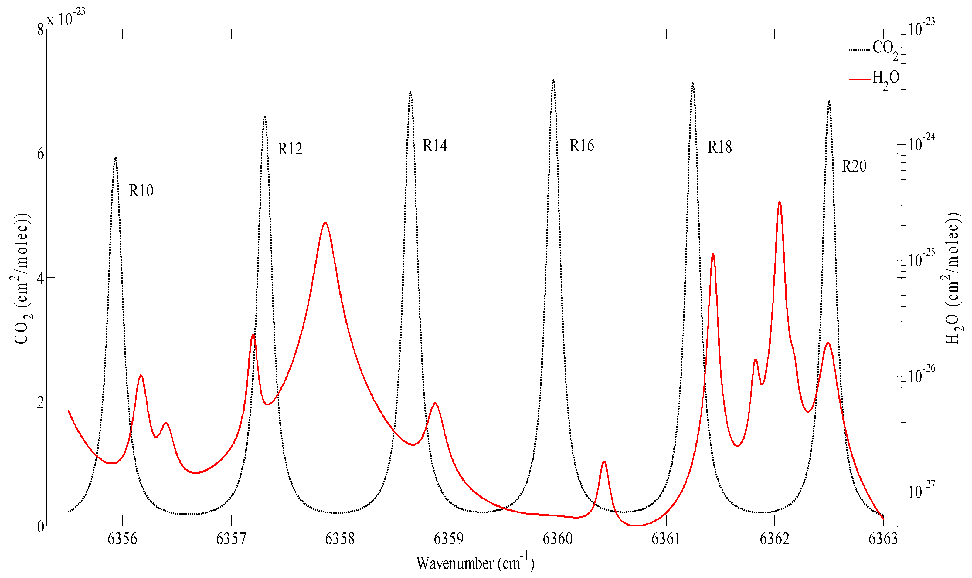
To evaluate the feasibility and accuracy of MW-DIAL for atmospheric CO₂ detection, we conducted a series of simulated experiments. Most spectroscopic parameters of CO₂ lines for the simulation analysis were obtained from Predoi-Cross et al. [28] and HITRAN 2012 [29]. The spectroscopic parameters of the absorption lines of H₂O were obtained from HITEMP 2010 [30,31]. According to the HITRAN 2012 molecular spectroscopic database, six absorption lines in the range of the 30012–00001 carbon-dioxide band were studied because their intensities were evidently higher than those of others. The spectroscopic parameters of the absorption lines of CO₂, which are marked as C1–C6 (namely, R10–R20), and those of H₂O in this range are listed in

Table 1. Spectroscopic parameters of CO₂ and H₂O involved in the simulation analysis.

Abb.	Position	Intensity	bL (Air)	E″	n	δ° (Air)	δ′ (Air)	P(pa)	T(K)
C1	6355.939	1.534 × 10−23	0.080	42.92	0.696	−4.59 × 10−3	−5.7 × 10−5	101325	296
C2	6357.312	1.661 × 10−23	0.078	60.87	0.695	−4.30 × 10−3	−7.0 × 10−5	101325	296
C3	6358.654	1.730 × 10−23	0.077	81.94	0.680	−4.92 × 10−3	−6.3 × 10−5	101325	296
C4	6359.967	1.741 × 10−23	0.075	106.13	0.672	−4.98 × 10−3	−8.3 × 10−5	101325	296
C5	6361.250	1.703 × 10−23	0.074	133.44	0.653	−5.60 × 10−3	−6.8 × 10−5	101325	296
C6	6362.504	1.621 × 10-23	0.073	163.87	0.693	−6.45 × 10−3	−6.5 × 10−5	101325	296
H1	6361.442	8.875 × 10−27	0.017	1327.12	−0.06	−0.0120	---	101325	296
H2	6356.177	1.469 × 10−27	0.048	1079.08	0.45	−0.0074	---	101325	296
H3	6355.156	3.130 × 10−26	0.060	586.48	0.34	−0.0060	---	101325	296
H4	6356.415	5.440 × 10−28	0.065	2919.63	0.44	−0.0127	---	101325	296
H5	6357.208	5.550 × 10−28	0.030	2254.28	0.01	−0.0090	---	101325	296
H6	6357.209	1.660 × 10−27	0.029	2254.28	0.01	−0.0094	---	101325	296
H7	6357.881	1.760 × 10−26	0.076	1899.01	0.59	−0.0195	---	101325	296
H8	6357.881	3.430 × 10−26	0.075	610.34	0.58	−0.0160	---	101325	296
H9	6358.894	1.090 × 10−27	0.074	2764.70	0.53	−0.0175	---	101325	296
H10	6361.838	1.020 × 10−27	0.025	2972.83	0.09	−0.0171	---	101325	296
H11	6362.055	2.550 × 10−26	0.018	1327.11	−0.06	−0.0120	---	101325	296
H12	6360.456	2.070 × 10−28	0.041	2927.94	0.37	−0.0273	---	101325	296
H13	6362.486	4.040 × 10−27	0.066	610.11	0.80	0.0020	---	101325	296

Position—Zero pressure line positions in cm⁻¹; Intensity—Line intensities in cm/molecule⁻¹ at 296 K; bL (air)—Air-broadened Lorentz width coefficients in cm⁻¹·atm⁻¹ at 296 K; E″—Lower-state energy in cm⁻¹; n—Temperature dependence exponents of air-broadened half-width coefficients (unitless); δ° (air)—Pressure-shift coefficients in cm⁻¹·atm⁻¹ at 296 K; δ′ (air)—Temperature-dependent coefficients of air-shift coefficients in cm⁻¹·atm⁻¹·K⁻¹.

. The absorption lines are also presented in Figure 2, with the absorption cross sections of the H₂O and CO₂ molecules at 101325 Pa and 296 K calculated using the Voigt profile. In spectroscopy, the Voigt profile is a line profile that results from the convolution of two broadening mechanisms. One of the broadening mechanisms produces a Gaussian profile as a result of the Doppler broadening; the other produces a Lorentz profile. Because of its physical implications, the Voigt function is superior to other functions for obtaining the absorption line of CO₂ [25]. The H₂O curve, which marks the right axis, is on a log scale, given that the intensities of the lines are much smaller than those of CO₂. H1–H13 were not labeled because our concern was their effects on CO₂. In selecting the operating wavelength, we had to consider many factors, such as low temperature sensitivity and low interference from other molecules. Previous studies showed that H₂O is the most critical interference molecule in the absorption spectroscopy of CO₂ [31,32]. As shown in Figure 2, R10, R12, and R20 are inappropriate because they are considerably affected by interferences from H₂O. R16 is the most appropriate because the intensity of this peak is the strongest, and the influence of H₂O in this band is less than that in R14 and R18. Consequently, less noise is generated, and the differential optical depth is the largest. Thus, R16 has the highest SNR in this range and is recommended for measuring atmospheric CO₂ using DIAL at 1572 nm.

4.1. Simulation Analysis of Wavelength Shift

The simulation analysis of wavelength shift was conducted in three parts. The first part concerned theoretical inversion, in which both the parameters of on-line and off-line wavelengths were theoretical values. Results of this inversion were supposed to be 400 ppm, which is marked as C₀ and used as the evaluation criterion for inversion. The logarithm of the energy ratio (i.e., DAOD) of on-line and off-line wavelengths was obtained using Equations (2) and (3). The DAOD was used for inversion in the second and third parts, which were both under the conditions of lasers with shifting wavelengths. The methods of inversion for the last two parts were DW-DIAL and MW-DIAL, respectively. The inversion results are marked as C₁ and C₂. Finally, C₀, C₁, and C₂ were compared to obtain the inversion accuracy of CO₂ using the different methods.

4.1.1. Part 1

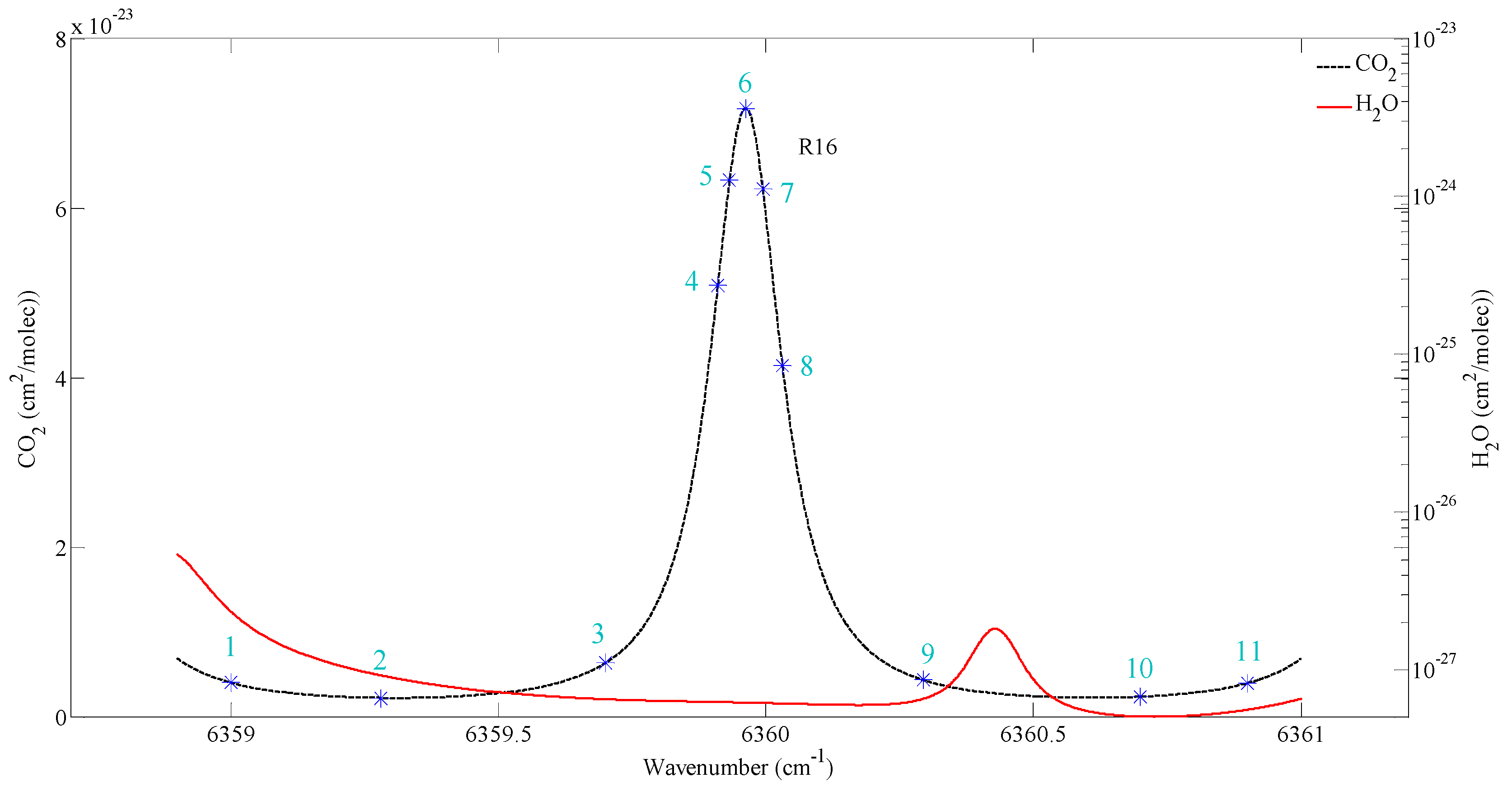
As shown in Figure 3, in the section of the on-line and off-line wavelengths in the region of R16, the on-line wavelength could be easily obtained because only one absorption peak of CO₂ was observed in the region of R16, which is marked as 2. The theoretical wavelength of point 2 was 6359.962 cm⁻¹. However, two absorption valleys of CO₂ were found on both sides of the on-line wavelength, which are marked as 1 and 3, respectively. According to the spectroscopic parameters of the CO₂ lines from HITRAN 2012, the intensity of Point 1 was lower than that of Point 3, but Point 1 was largely affected by the water vapor. The intensity of water vapor at Point 1 was approximately 8.9162 × 10⁻²⁸ whereas that at Point 3 was 5.4435 × 10⁻²⁸. Consequently, Point 3 was considered to be the position of the off-line wavelength, and its wavelength was 6360.609 cm⁻¹.

According to Section 2, the DAOD of the on-line and off-line wavelengths could be easily obtained through the DW-DIAL: supposing that r₁ = 0, r₂ = 50, P(λ_on, r₁) = P(λ_off, r₁) = 4 mJ, C₀ = 400 ppm. In addition, σ_g(λ_on) and σ_g(λ_off) could be obtained from HITRAN 2012, which were 7.1785 × 10⁻²³ and 2.2250 × 10⁻²⁴ cm², respectively. Then, N₀ = 1.0747 × 10²², and $\text{DAOD}=\text{ln}\frac{P\left({\mathsf{\lambda }}_{off},r_2\right)}{P\left({\mathsf{\lambda }}_{on},r_2\right)}$ = 7.476 × 10⁻³ for the on-line and off-line wavelengths of DW-DIAL based on Equations (2) and (3).

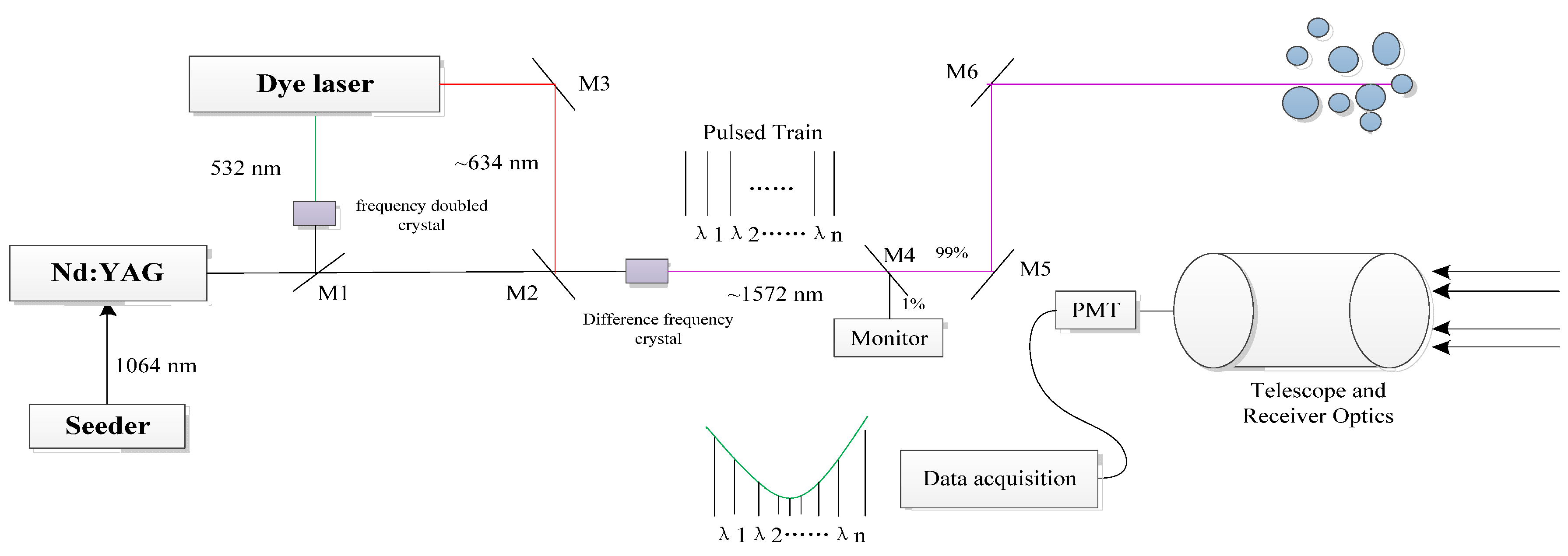
In the system of MW-DIAL, the number and position of multiple wavelengths were various and could be adjusted according to the situation. The general concept here is that all points are distributed on both sides of the absorption peak. Points close to the absorption peak are relatively dense, whereas those away from the absorption peak are sparse. In this study, 11 points were selected for the simulated experiments using MW-DIAL. Their positions are shown in Figure 4.

The calculation of DAOD for MW-DIAL is similar to that for DW-DIAL. In this study, the points distributed on both sides of the absorption peak were regarded as the off-line wavelengths and used in the difference processing with the on-line wavelength. DAODs of the on-line and each off-line wavelength were obtained according to Equations (2) and (3), which are listed in

Table 2. Parameters of the selected points in the MW-DIAL.

λ (cm−1)	σ (cm2)	DAOD
6359.000	4.0309 × 10−24	7.282 × 10−3
6359.280	2.2087 × 10−24	7.478 × 10−3
6359.700	6.3319 × 10−24	7.035 × 10−3
6359.910	5.0866 × 10−23	2.248 × 10−3
6359.932	6.3286 × 10−23	9.135 × 10−4
6359.962	7.1785 × 10−23	0.0000
6359.994	6.2279 × 10−23	1.022 × 10−3
6360.031	4.1391 × 10−23	3.267 × 10−3
6360.295	4.3222 × 10−24	7.251 × 10−3
6360.700	2.3463 × 10−24	7.463 × 10−3
6360.900	3.9719 × 10−24	7.288 × 10−3

.

4.1.2. Part 2

Part 2 involved the analysis of inversion through DW-DIAL under the condition of lasers with shifting wavelengths. Supposing that the shift of on-line and off-line wavelengths was 1 pm, which is approximately 0.004 cm⁻¹ in the region of R16, the absorption cross sections of on-line and off-line wavelengths became σ_g(λ_on) = 7.1785 × 10⁻²³cm² and σ_g(λ_off) = 2.2250 × 10⁻²⁴cm² from HITRAN 2012. However, they were still considered to be located at the absorption peak and valley, and their original values were used in the inversion. Accordingly, an error result in the inversion was produced. The inversion errors of different shifts of wavelength in the DW-DIAL are listed in

Table 3. Inversion error analysis of different shifts of wavelength in the DW-DIAL.

Δλ (pm)	Direction	λ (cm−1)		σ (cm2)		n	C (ppm)
		λ(on)	λ(off)	σ(on)	σ(off)
0		6359.962	6360.609	7.1785 × 10−23	2.2250 × 10−24	1.0747 × 1022	400.00
1	R	6359.966	6360.613	7.1619 × 10−23	2.2252 × 10−24	1.0722 × 1022	399.04
	L	6359.958	6360.605	7.1615 × 10−23	2.2252 × 10−24	1.0721 × 1022	399.02
2	R	6359.970	6360.617	7.1118 × 10−23	2.2259 × 10−24	1.0644 × 1022	396.16
	L	6359.954	6360.601	7.1112 × 10−23	2.2258 × 10−24	1.0643 × 1022	396.12
5	R	6359.982	6360.629	6.7781 × 10−23	2.2307 × 10−24	1.0128 × 1022	376.94
	L	6359.942	6360.589	6.7766 × 10−23	2.2305 × 10−24	1.0126 × 1022	376.85
7	R	6359.990	6360.637	6.4296 × 10−23	2.2362 × 10−24	9.5885 × 1021	356.87
	L	6359.934	6360.581	6.4277 × 10−23	2.2358 × 10−24	9.5856 × 1021	356.76
9	R	6359.988	6360.645	6.0128 × 10−23	2.2436 × 10−24	8.9435 × 1021	332.86
	L	6359.926	6360.573	6.0107 × 10−23	2.2430 × 10−24	8.9402 × 1021	332.74

. The shifts of on-line and off-line wavelengths were 1, 2, 3, 7, and 9 pm, respectively. Note from Table 3 that the inversion error increases rapidly as the shift of on-line and off-line wavelengths increases. In addition, the errors caused by wavelength shift in the left direction are greater than those in the right direction. This is probably because of the difference between the left and right parts of the CO₂ absorption line.

4.1.3. Part 3

Part 3 involved an analysis of inversion through MW-DIAL under the condition of lasers with shifting wavelengths. This analysis processing was similar to that in Part 2. Supposing a shift of on-line and off-line wavelengths occurred in the region of R16, causing a change in the absorption cross sections of multiple wavelengths. However, they were still considered to be located at the original positions, and their original values were used in the inversion. Accordingly, an error in the inversion was produced.

Given the many points that participate in the inversion, all parameters of the points are not listed. For Part 3 of the simulation, a list of only the final inversion results is shown in

Table 4. Inversion error analysis of different shifts of wavelength in the MW-DIAL.

Δλ (pm)		0	1	2	5	7	9
C (ppm)	R	400.00	399.56	397.83	383.68	364.77	336.42
	L		399.22	397.21	383.14	365.78	340.47

.

As shown in Table 3 and Table 4, given the drifting wavelengths of the laser, the detection accuracy of MW-DIAL for CO₂ was higher than that of DW-DIAL, especially when the drift was large.

4.2. Simulation Analysis of Different SNRs

In addition, we have also analyzed the inversion precision of two methods with echo signal of different SNRs to evaluate the feasibility and accuracy of MW-DIAL for atmospheric CO₂ detection. The simulation analysis of different SNRs was conducted in two parts.

4.2.1. Part 1

For the DW-DIAL, echo signal of on-line and off-line wavelengths with a range of 5 km was simulated for the analysis, which is shown in Figure 5. The initial CO₂ concentration was assumed to be 400 ppm, and the temperature and pressure profiles were obtained by interpolating the sounding data of the temperature and pressure. Compared with the off-line wavelength, the on-line wavelength fell more rapidly due to CO₂ absorption. When dealing with pure signals, DAOD was calculated based on the signal intensity of on-line and off-line wavelengths. Then the difference of absorption cross of on-line and off-line wavelengths which was used in the following analysis could be obtained by Equation (4).

The Gaussian noise was added to the simulated echo signal, and the echo signals of LIDAR with different SNRs are shown in Figure 6 and Figure 7.

In the simulation analysis of different SNRs, the errors of DAOD of on-line and off-line wavelengths were caused by the noises, including the background noise, thermal noise, and so on. The DAODs of LIDAR with different SNRs are shown in the Figure 8 and Figure 9, corresponding to the SNR of 80, 50, 30 and 10.

The integrated concentration of CO₂ in the range of 5 km was calculated by the inversion formula and compared with the initial concentration of CO₂ to obtain the inversion accuracy of CO₂ in different noise levels by DW-DIAL. In order to avoid the occasionality of one experiment, a total of 100 simulated experiments was performed and the mean value was considered as the inversion value for each SNR. The inversion results of different SNRs by DW-DIAL are listed in the

Table 5. The inversion results of different SNRs by DW-DIAL (unit: ppm).

	SNR = 80	SNR = 60	SNR = 30	SNR = 10
C	398.9184	395.5462	417.2130	34.3637

.

4.2.2. Part 2

For the MW-DIAL, the process of simulated analysis is similar to that of DW-DIAL. The simulated signal of MW-DIAL is shown in Figure 10. To obtain the echo signals of LIDAR with different SNRs, the Gaussian noise was added. Considering the existence of 11 wavelengths, echo signals with different SNRs were not shown in this part, while the final inversion results are shown in

Table 6. The inversion results of different SNRs by MW-DIAL (unit: ppm).

	SNR = 80	SNR = 60	SNR = 30	SNR = 10
C1	400.2770	399.4180	424.4756	−79.7033
C2	399.8802	398.1945	419.0777	217.3927
C3	399.9982	398.2993	422.2781	166.8717
C4	399.3138	391.1946	384.7474	291.2483
C5	399.0247	405.1858	418.5221	179.0400
C6	401.2253	401.0512	419.3369	138.6330
C7	400.3320	399.7971	427.6594	−135.2407
C8	399.9275	396.4240	383.7268	267.6911
C9	400.3947	386.4913	388.8763	210.3033
C10	400.1776	403.4622	397.0623	88.2754
C	400.1068	396.9957	406.1931	139.2494

.

The integrated concentration of CO₂ in the range of 5 km was calculated by the inversion formula and compared with the initial concentration of CO₂ to obtain the inversion accuracy of CO₂ in different noise levels by MW-DIAL. Similarly, in order to avoid the occasionality of one experiment, a total of 100 simulated experiments was performed and the mean value was considered as the inversion value for each SNR. The inversion results are shown in Table 6: C1–C10 are the inversion results of on-line wavelength and each off-line wavelength, respectively; C is the final inversion result by MW-DIAL.

The concentration of CO₂ obtained by the two methods and the difference with initial concentration (d-C for short) are listed in the

Table 7. Comparison of the inversion results by DW-DIAL and MW-DIAL (unit: ppm).

		SNR = 80	SNR = 60	SNR = 30	SNR = 10
C	DW-DIAL	398.9184	395.5462	417.2130	34.3637
	MW-DIAL	400.1068	396.9957	406.1931	139.2494
d-C	DW-DIAL	1.0816	4.4538	17.2130	365.6363
	MW-DIAL	0.1068	3.0043	6.1931	260.7506

. It can be noted that the inversion accuracy of MW-DIAL was better than that of DW-DIAL, especially for the signal with low SNR. In addition, there was an unacceptable inversion error for both methods while the SNR was lower than 30, thus it is necessary to eliminate the noise in the signal processing.

5. Experiments with Laboratory Signal

Considering that our instruments did not have the capability of multi-wavelength atmospheric sounding because of the slow wavelength conversion speed at this stage, experiments through a gas absorption cell with a range of 16 m were conducted to test the feasibility and accuracy of the inversion algorithm. CO₂ with a purity of 100% was filled into the gas absorption cell, and the concentration of CO₂ was used as the evaluation standard for inversion. The temperature and pressure of the gas absorption cell was 323 K and 1 atm, respectively. Lasers with different wavelengths were coupled through the optical fiber. The OD was obtained using a high-precision sampling oscilloscope and the LabVIEW program. The concentration of CO₂was calculated through the inversion algorithm with DAOD and absorption cross section from HITRAN 2012 in the laboratory experiments.

The process was similar to the simulation experiments. In the simulation experiments, DAODs were obtained by the concentration and absorption cross section from HITRAN 2012. Wavelength drifts were then added to the inversion to calculate the concentration of CO₂. The inversion accuracy was evaluated by comparing the calculated value with the truth concentration. In the laboratory experiments, DAODs of different wavelengths were obtained by the gas absorption cell and high-precision sampling oscilloscope. The concentration was then calculated with DAODs and absorption cross section from HITRAN 2012. The inversion accuracy was evaluated by comparing the calculated value with the real concentration of CO₂ in the gas absorption cell. Wavelength drift always exists in laboratory experiments, which can be monitored using a high-precision wavemeter.

In this study, LIDAR signal was normalized by a dual-differential method using two absorption cells. The system configuration of the wavelength control unit is shown in Figure 11. Eight percent of the pulsed laser lights transmitted from the laser system was used as the laser source of the wavelength control unit. The laser was then tapped to 90:10 using a one-sided antireflection-coated glass, which is marked as M1 in Figure 11. The lights of the 10% were transmitted to a wavemeter as part of the laser source of coarse calibration, and those of the remaining 90% were split by half using a half-reflector, which is marked as M2. Two identical laser lights were then transmitted to the 16-m absorption cells: one was filled with pure CO₂ and the other was a vacuum. Both lights transmitted through the 16-m absorption cell were detected by an infrared detector, and the laser intensity was collected by an oscilloscope, in which the trigger signal derived from the laser system. The connecting lines marked as 1, 2, and 4 in Figure 11 are bayonet nut connectors, whereas those marked as 3, 5, and 6 are commercial cables. The absorption line of CO₂ could be obtained through the ratio of the intensity of the laser of the two branches.

In the laboratory experiments of DW-DIAL, the absorption spectra of CO₂ was first obtained using a gas cell with a large scale of approximately 10 pm, and the absorption spectra of CO₂ at the region of R16 was located using a wavemeter whose accuracy was approximately 5 pm. After locating R16, we conducted a fine scanning at a step size of 3 pm and obtained the location of the on-line wavelength using a wavelength stabilization program, about which a detailed introduction is in [25]. The laser of the on-line wavelength was then imported into the gas absorption cell of the 16-m range, and the OD was obtained using the oscilloscope, following the collection procedures. The location of the off-line wavelength was determined by means of λ_off = λ_on − 0.1599 um, which confirms with the distance between the on-line and off-line wavelengths from HITRAN 2012. The laser of the off-line wavelength was then imported to the gas absorption cell of the 16-m range, and the OD was obtained. Finally, the DAOD of the on-line and off-line wavelengths and their absorption cross section at the region of R16 from HITRAN 2012 were inserted into the inversion equation. Thus, the concentration of CO₂ in the gas absorption cell could be calculated. Here, the calibration of the bandwidth [33] must be the focus of attention.

In the laboratory experiments of MW-DIAL, the absorption spectra of CO₂ was first obtained using a gas cell with a large scale, and the absorption spectra of CO₂ at the region of R16 was located using a wavemeter. After locating R16, we selected 11 points according to the general principle of multiple point selection. The laser of different wavelengths was then imported into the gas absorption cell of the 16-m range, and the ODs were obtained using the oscilloscope, following the collection procedures. Finally, the DAODs of the on-line and off-line wavelengths and their absorption cross section at the region of R16 from HITRAN 2012 were plugged into the inversion equation. Accordingly, the concentration of CO₂ in the gas absorption cell was obtained.

Finally, the concentration of CO₂ in the gas absorption cell and the concentration of CO₂ detected through the DW-DIAL and MW-DIAL were compared to evaluate the inversion precision of the two methods. The ODs of different wavelengths and inversion results are shown in

Table 8. Optical depths of different wavelengths and inversion results using the two methods.

Method	Point	OD	DAOD	σ (cm2)	C (%)
DW-DIAL	on	1.4686	0.8193	7.1785 × 10−23	108.0469
	off	0.6493		2.2250 × 10−24
MW-DIAL	on	1.4686		7.1785 × 10−23	Ci (i = 1, 2, …, 10)	$\frac{B_1^2{C}_1+B_2^2{C}_2+\dots B_{10}^2{C}_{10}}{B_1^2+B_2^2+\cdots +B_{10}^2}$ = 98.4796
	off_1	0.4836	0.9851	4.0309 × 10−24	133.3629
	off_2	0.4877	0.9810	2.2087 × 10−24	129.3323
	off_3	0.8247	0.6439	6.3319 × 10−24	90.2427
	off_4	1.2191	0.2495	5.0866 × 10−23	109.4096
	off_5	1.3704	0.0982	6.3286 × 10−23	106.0325
	off_6	1.4268	0.0418	6.2279 × 10−23	40.3660
	off_7	1.1633	0.3053	4.1391 × 10−23	92.1497
	off_8	0.8680	0.6007	4.3222 × 10−24	81.6761
	off_9	0.7486	0.7200	2.3463 × 10−24	95.1179
	off_10	1.0231	0.4455	3.9719 × 10−24	60.2624

.

Table 8 reveals that the detection accuracy of CO₂ through MW-DIAL is higher than that through DW-DIAL, given that the wavelengths of the laser were drifting.

6. Conclusions

In this study, an MW-DIAL was proposed for accurate detection of atmospheric CO₂ using a pulsed laser. The method conducts the inversion with one on-line and multiple off-line wavelengths. A feasibility study of MW-DIAL for CO₂ monitoring from the inversion algorithm was analyzed. The least square method was used to optimize inversion results and the inversion concentration of CO₂ in the MW-DIAL system was found to be the weighted average of the multiple concentrations. In addition, the single on-line and multiple off-line wavelengths were obtained through multi-wavelength scanning, which involves continuous sampling across the CO₂ absorption line with an appropriate number of points and range of widths. The complete absorption line of CO₂, including the absorption peak and valley, could be obtained through curve fitting. This method avoids the strict locking of the on-line wavelength and therefore improves the precision of CO₂ detection.

Simulation analysis and laboratory experiments were conducted to evaluate the inversion precision of the two methods. The simulation analysis of wavelength drift demonstrated that—given the drifting wavelengths of the laser—the detection accuracy of CO₂ through MW-DIAL was higher than that through DW-DIAL, especially when the drift was large. In addition, simulated experiments indicated that wavelength stabilization is necessary in both DW-DIAL and MW-DIAL systems. However, the requirements of wavelength stabilization are more relaxed in an MW-DIAL system, which results in a more accurate detection of CO₂. In the simulation analysis of different SNRs, the inversion accuracy of MW-DIAL was better than that of DW-DIAL, especially for the signal with low SNRs. A laboratory measurement was also performed to verify our simulation analysis. The errors of inversion results in a gas absorption cell were 8.0469% and 1.5204% through DW-DIAL and MW-DIAL, respectively.

The method of MW-DIAL compensates for the deficiency of stringent wavelength accuracy and stability required in a DW-DIAL system. In addition, MW-DIAL can also reduce the errors affected by other factors, such as atmospheric temperature, pressure, and the baseline variation of wavelengths.

Although the MW-DIAL has obvious advantages such as high precision and relaxed requirements of wavelength stabilization, the requirements of hardware and the receiving system are high, and the occupied space and cost are more than those of DW-DIAL. Directions for future research on MW-DIAL include the miniaturization of the laser transmitter and the development of a receiving system. In addition, in the real experiments of CO₂, some errors may arise because of real atmospheric situations occurring under varying meteorological conditions.