
Coherent Momentum Exchange above and within a Scots Pine Forest

Environmental Meteorology, Albert-Ludwigs-University of Freiburg, Werthmannstrasse 10, Freiburg D-79085, Germany
*
Author to whom correspondence should be addressed.
Atmosphere 2016, 7(4), 61; https://doi.org/10.3390/atmos7040061
Submission received: 20 January 2016
/
Revised: 13 April 2016
/
Accepted: 18 April 2016
/
Published: 21 April 2016
Abstract
:Biorthogonal decomposition (BOD) is used to detect and study synchronous coherent structures occurring at multiple levels in the vertical momentum flux () within and above a planted Scots pine forest during a 12-week continuous measurement period. In this study, the presented method allowed for the simultaneous detection and quantification of the number of coherent structures (N), their duration (D) and separation (S) at five measurement heights (z1–z5) covering the range z1/h = 0.11 to z5/h = 1.67, with h being the mean stand height at the measurement site. Results presented for five different exchange regimes (C1–C5) and for four different atmospheric stability conditions (stable, transition to stable, near-neutral, forced convection) demonstrate that during the measurement period, above-canopy momentum flux was only to a limited extent involved in the evolution of spatiotemporal momentum flux patterns found within the below-canopy space. Fully-coupled turbulent momentum exchange over the investigated height range occurred during 19% of all analyzed half-hourly datasets. Across the analyzed exchange regimes, the median contribution of strong sweeps and ejections to total momentum transfer above the canopy varied between 30% and 39% while covering 28%–32% of the time. In the below-canopy space, the contribution of coherent structures varied between 19% and 21% while covering the same amount of time. This suggests that momentum transfer through synchronous coherent structures is very efficient above the forest canopy, but attenuated in the below-canopy space. Since the majority of the presented results agrees well with the results from previous studies that analyzed coherent structures at single levels, the BOD is a promising tool for the consistent investigation of synchronous coherent structures at multiple measurement heights.
1. Introduction
Various methods have been applied to detect and investigate strong, organized turbulent structures that intermittently exchange substantial amounts of heat, mass, momentum and other scalar quantities between plant canopies and the roughness sublayer located directly above them [1]. These structures are often referred to as coherent structures, because their characteristics appear coherently at several levels within and above plant canopies [2,3] and can be separated from weaker, small-scale fluctuations in turbulent flow [4]. Two quantitative methods, which have been most commonly applied to investigate coherent structure characteristics in data measured in the field, are quadrant analysis [5,6] and wavelet analysis [7,8,9]. As can be expected, there are considerable differences between these methods in their coherent structure detection capabilities [7,10]. Furthermore, the definition of coherent structures varies in previous studies, which introduces differences in coherent structure properties [11].
Although the same coherent structures are detected at several levels within and above forest canopies, results from previous studies that applied quadrant and/or wavelet analysis were often reported from single-level evaluations [12,13,14]. Wavelet analysis requires the determination of peak scales, which are derived from the measurements at each height separately [15]. This can pose a problem when investigating coherent structures that occur simultaneously at several heights, since different peak scales introduce differences in the appearance of coherent structures. In a recent study, the wavelet analysis was used to evaluate synchronous coherent structures at two different measurement heights by introducing time offsets between the heights [16]. Thus, for the investigation of coherent structure characteristics, it is more desirable to have a method that extracts structures from time series that are occurring at multiple heights simultaneously. Then, the spatiotemporal evolution and propagation of coherent structures could consistently be analyzed over the height range covered by the airflow measurements.
Since tower-based micrometeorological measurements in plant canopies are mainly carried out in the canopy layer and in the roughness sublayer, which extends up to two or three canopy heights [17], there is a great interest in improving the interpretability of the dynamics of coherent structures when moving through plant canopies and in quantifying the contribution of coherent structures to total turbulent canopy-atmosphere exchange. This is important when chemical concentration gradients [18,19] and turbulent carbon and energy fluxes are measured within and above plant canopies [20] to study and model matter and energy cycles. A better understanding of coherent structure propagation into forest canopies is also of importance when tree response to wind loading is investigated [21,22].
To gain a deeper understanding of the spatiotemporal evolution and propagation of coherent structures above and within tall plant canopies, it is necessary to detect and separate coherent structures from small-scale turbulence [14]. A method that allows for this separation, as well as for the simultaneous analysis of several time series is the biorthogonal decomposition (BOD) [23]. The BOD is able to capture important common time-space characteristics in high-dimensional datasets. In the field of plant canopy turbulence, the BOD has already successfully been applied in previous studies focusing on the detection of coherent patterns in the interactions of airflow and plant canopies [22,24,25].
The objectives of this study are to investigate the spatiotemporal evolution of synchronous coherent structures occurring in the vertical turbulent momentum flux within and above a planted Scots pine forest canopy and to quantify their typical characteristics under different atmospheric stability conditions and exchange regimes. For that purpose, the BOD is applied on wind vector component time series, which were measured at five levels within and above a Scots pine plantation canopy.
2. Material and Methods
2.1. Measurement Site
Airflow measurements were carried out at the forest research site Hartheim, which is located approximately 25 km southwest of Freiburg (southwest Germany) in the flat southern Upper Rhine Valley (47°56′04″N, 7°36′02″E, 201 m above sea level). The research site was operated for more than 40 years by the Meteorological Institute of the University of Freiburg. The forest at the measurement site is a single-layered Scots pine (Pinus sylvestris L.) plantation, which was established in the 1960s. In the year 2014, the forest’s mean height (h) was approximately 18 m, and its mean stand density around the measurement site was 580 trees·ha−1. The mean plant area index (PAI) is 1.5. Figure 1a shows the normalized plant area density (PAD) profile at the measurement site.
2.2. Airflow Measurements
During the period from 3 June 2014–25 August 2014, the wind vector components in the x- (u), y- (v) and z-direction (w) were measured (sampling rate: 10 Hz) above and within the forest canopy using five ultrasonic anemometers (R.M. Young Company, Type 81000VRE). The ultrasonic anemometers were mounted on a 30 m high lattice tower at 2 m (z1/h = 0.11), 9 m (z2/h = 0.50), 18 m (z3/h = 1.00), 21 m (z4/h = 1.15) and 30 m (z5/h = 1.67) above ground level (a.g.l.). Since airflow from northern and southern directions dominates at the measurement site (>90% during the measurement period; Figure 1b), the ultrasonic anemometers were oriented to the west on 1.5 m-long supporting booms to minimize the influence of the tower on the wind measurements. Furthermore, all data from eastern directions were excluded from the analysis. During the measurement period, half-hourly wind speed was lower than 5.0 m·s−1 over 98% of the time. The maximum 30-min mean wind speed value at z5 was 9.1 m·s−1.
2.3. Data Processing
First of all, the 1750 available half-hourly time series of wind vector data were despiked with a one-step procedure. The despiking method analyzed the mean and standard deviation for each 300-s window. Spikes were defined as values with an amplitude of at least 3.5 standard deviations away from the 300-s median values. If spikes were detected, then they were replaced by the corresponding values of a median filtered version of the time series. For a better comparison with previous studies, a double rotation was applied on the wind vector data to align the x-axis of the wind vector coordinate system into mean wind direction and to set the mean lateral and vertical wind vector components to zero [26,27]. The data of all measurement heights were rotated according to the rotation angles derived from the data at z5 to ensure that the same coordinate system was used for all time series. After that, Reynolds decomposition was used to split the rotated wind vector components into mean (denoted by an overbar) and turbulent parts (denoted by a prime).
To highlight coherent, organized structures in the wind vector component time series, a band pass infinite impulse response (IIR) filter was used to smooth out short-term fluctuations and eliminate low-frequency parts. Based on previous results on the typical duration of coherent structures in and above the Scots pine forest [22], the cut-off frequencies chosen to separate coherent structures from long-term variations and short-term fluctuations were 0.003 Hz and 0.05 Hz. Thus, the filter removes all variations longer than 300 s and also all fluctuations smaller than event durations of 20 s from the and time series. The cut-off frequencies were found to be suitable to include all relevant temporal scales associated with coherent flux structures.
2.4. Classification of Atmospheric Stability
The classification of atmospheric stability was based on half-hourly values of the Obukhov length Λ [28], which was calculated according to [29]:
with the virtual potential temperature θv, the friction velocity , the von Kármán constant κ = 0.4 and the gravitational acceleration g = 9.81 m·s−1. Following [30], the variations of heat and momentum flux were analyzed as a function of the canopy-top stability parameter to determine the boundary values for for the different atmospheric stabilities. Then, all available half-hourly datasets were assigned to the six derived stability classes listed in Table 1.
It has to be noted that theoretically, Λ is not applicable over heterogeneous surfaces. However, Λ calculated above forest canopies still approximates the prevalent atmospheric stability conditions reasonably well and is therefore widely used for non-ideal surfaces, as well.
An interval length of 30 min might have an effect on within-canopy turbulent exchange under stable conditions [6,31]. Therefore, frequency characteristics of and time series were compared under different stability conditions using Fourier analysis. Since no stability-dependent, deterministic differences in Fourier spectra were found, 30 min was used as the interval length under all stability conditions. Following [32], all datasets classified as very stable and free convection were excluded from further analysis.
2.5. Wavelet Analysis
In a number of previous studies that focused on the detection and analysis of coherent structures as part of turbulent exchange processes through plant canopies, wavelet analysis was applied [7,8,33,34]. In comparison to Fourier transform, the wavelet transform shows good resolution in both frequency and time domains, which is achieved by decomposing a time series with a family of wavelet functions. The wavelet functions are produced by dilatation and translation of a mother wavelet ψn,s(t) [35]:
with n being the translation parameter, which corresponds to the position of the wavelet on the time axis, and s is the scale dilatation parameter, which corresponds to the width of the wavelet function. Wavelet functions that are commonly used in plant canopy turbulence analysis include the Mexican hat wavelet [7,8,11,12,34,36], the complex Morlet wavelet [32,33,37] or the Haar wavelet [13,36].
The continuous, one-dimensional wavelet transform of a time series f(t) is defined as the convolution of f(t) with ψn,s(t) [35]:
where Cn(s) are the wavelet coefficients. The wavelet variance W(s), i.e., the amount of signal energy contained at s, can be calculated as follows [11]:
Calculating W(s) over all scales yields the wavelet variance spectrum. From analysis of its maxima (W(speak)), the peak scale speak corresponding to the typical duration of coherent structures can be detected [38]. The wavelet coefficients Cpeak associated with W(speak) are used for further analysis. The zero-crossings of these coefficients allow the detection of abrupt changes in time series, which are commonly used to detect individual coherent structures [7,8,11,12,39].
To each s, a corresponding Fourier-equivalent frequency (Fa) and, thus, a corresponding time scale, can be calculated from the center frequency Fc of the used wavelet and the sampling frequency Δ [40]:
The detection method for coherent structures presented in this paper was compared to wavelet analysis. For this comparison, the Mexican hat (MH) wavelet was used to detect coherent structures in half-hourly and time series, because it is well-localized in time [8]. MH-coefficients were calculated for the scales 50–750, which correspond to time periods from 20–300 s. If W(s) showed several prominent peaks, then the peak scale corresponding to the shortest period was assumed to be associated with coherent structures [12].
2.6. Biorthogonal Decomposition
To investigate coherent structures in the momentum flux that are common to more than one measurement height, a method is desired that detects coherent structures in airflow time series over several heights simultaneously. The comparison of results from wavelet analysis over several heights is not always straightforward because height-specific speak may not always be the same, leading to a different coherent structure appearance at every height.
The method that is proposed for simultaneous detection of coherent structures over several heights is the biorthogonal decomposition (BOD) [23]. For the application of the BOD, the time series are compiled into space-time signals on (X × T) with X being the set of measurement points in space and T being the corresponding measurement times to each measurement point. It can be expressed as:
with k being the number of BOD components, are weighting factors, λk are roots of the eigenvalues, µk(t) are temporal modes, νk(x) are spatial modes and (νk(x), µk(t)) form a set of normalized orthogonal functions. It was demonstrated that the eigenmodes of the spatial operator:
are spatial modes with the corresponding eigenvalues λk [23]. The asterisk indicates the complex conjugate of . The eigenmodes of the temporal correlation operator:
are temporal modes with the same set of eigenvalues λk. By multiplication with , the spatial information of the signal can be separated from its temporal information [23,41]. Since the norm of the series converges, it is possible to truncate the series to the first k terms [23].
The total energy of the analyzed signals is defined as [41]:
The explained variance of each k-th term in the series , called the relative eigenvalue λrk, can be calculated according to [41]:
Information about phase lags in time and space between the time series of are contained in the different behavior of the chronos and topos [24,25,41].
In this study, the BOD is applied to the turbulent wind vector components :
Since wind vector components were measured at five levels, the BOD yields a maximum of five components after the decomposition of .
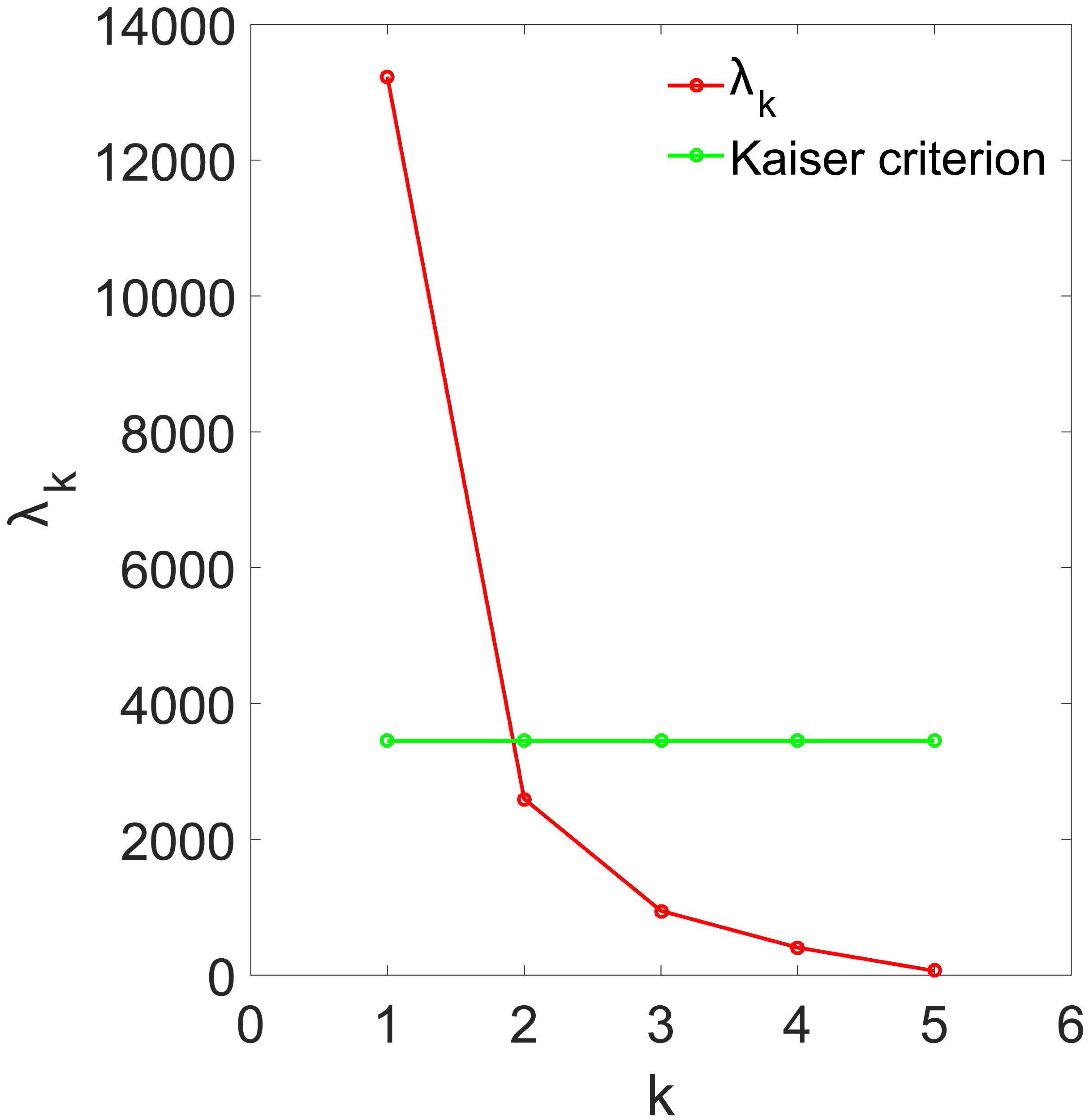
The main purpose of the application of the BOD is to reduce the dimensionality of . Normally, not all five BOD components contain information that is useful for the detection of coherent structures in the time series. Therefore, the number of useful BOD components derived from the and time series was determined for every 30-min interval by analyzing scree plots [42]. Here, scree plots show BOD component-specific eigenvalues as a function of the number of BOD components. The Kaiser criterion [43], which is defined as the mean value of all eigenvalues, was used to determine the number of useful BOD components of . The example shown in Figure 2 leads to one relevant BOD component that is used for the reconstruction. Every BOD component with an eigenvalue larger than the Kaiser criterion was considered to contain useful information and was used to reconstruct decomposed :
The reconstructed half-hourly time series were then used to calculate time series:
Based on the time series, characteristics of coherent structures in turbulent momentum exchange through the forest canopy were analyzed.
2.7. Classification of Exchange Regimes
Following [33], five exchange regimes (C1–C5) were defined that enable the case-by-case detection of patterns that form when coherent structures propagate through the height range covered by the airflow measurements. Overall, 16 combinations of momentum flux information are possible (Table 2). These combinations were assigned to C1–C5 based on the absolute value of the Pearson correlation coefficient (R), which was calculated between time series of adjacent heights for all half-hourly intervals. After evaluating different R-thresholds, reconstructed momentum flux was defined to be coupled between two adjacent measurement heights when R ≥ 0.8. The measurement height z5 is considered as the origin of the penetration depth of coherent structures.
If only one BOD component is used to build and , then it follows that |R| = 1 between all heights. This is due to the fact that only the absolute values of and change. If the calculation of either or involves more than one BOD component, then |R| < 1.
Applying this correlation criterion, C1 corresponds to all half-hourly time series at z1–z4 that are uncoupled with time series at z5. If C5 is detected, then is fully coupled from z5–z1.
2.8. Detection and Classification of Coherent Structures
Similar to quadrant analysis, coherent structures were detected when local variations fell below – H , with H = 3 to consider only strong events [6,44]. Detected coherent structures were classified according to the conventions of quadrant analysis based on the signs of and [5,45,46]: sweep (+, −) and ejection (−, +).
After coherent structure detection, the signs of and associated with individual coherent structures were determined after zero-crossings of and classified as sweep or ejection. The number (Nmeas) of coherent structures, their duration (Dmeas) and separation (Smeas) were determined for all half-hourly intervals. To account for bias in Nmeas, Dmeas and Smeas values obtained under atmospheric stability conditions with generally lower wind speed (stable, transition to stable, forced convection), all values are normalized. The normalization factor β is calculated as the ratio between the mean wind speed and the mean wind speed under near-neutral conditions : . Since Nmeas values are smaller due to lower wind speed, Nmeas is normalized as follows:
Dmeas and Smeas values are multiplied by β since Dmeas and Smeas are larger due to lower wind speed:
Typical coherent structure characteristics are presented by median values (, , ) and the interquartile range (IQR) in order to provide robust estimation of the central tendencies in the total number of coherent structures. The Wilcoxon rank sum (WRS) test [47] was used to evaluate whether there is a significant difference (level of significance α = 0.05) in coherent structure properties determined for different heights, coherent structure types, exchange regimes and stability conditions.
Using Taylor’s hypothesis of frozen turbulence [48], the length scale L of a coherent structure can be obtained by:
with being the convective velocity [5] and being the mean wind speed at canopy height; is the mean normalized duration of a detected coherent structure.
The contribution of sweeps to the overall turbulent momentum exchange (Fcoh,sw) and the contribution of ejections to the overall turbulent momentum exchange (Fcoh,ej) were calculated as follows [13]:
where nsw is the number of detected sweeps, nej is the number of detected ejections, mi is the number of continuous 10-Hz time series of during the i-th detected coherent structure and Ntot is the total number of measurement points in a 30-min interval. Then, the total contribution of both, sweeps and ejections, to the overall turbulent momentum exchange was calculated:
The exchange efficiency E was calculated from half-hourly Fcoh [11]:
with C being the net time cover of all coherent structures, which was calculated by:
where T = Ntot/10 Hz and Di is the duration of the individual coherent structure i.
Furthermore, the attenuation A of the amplitude at zi was calculated for every coherent structure n detected at height z5:
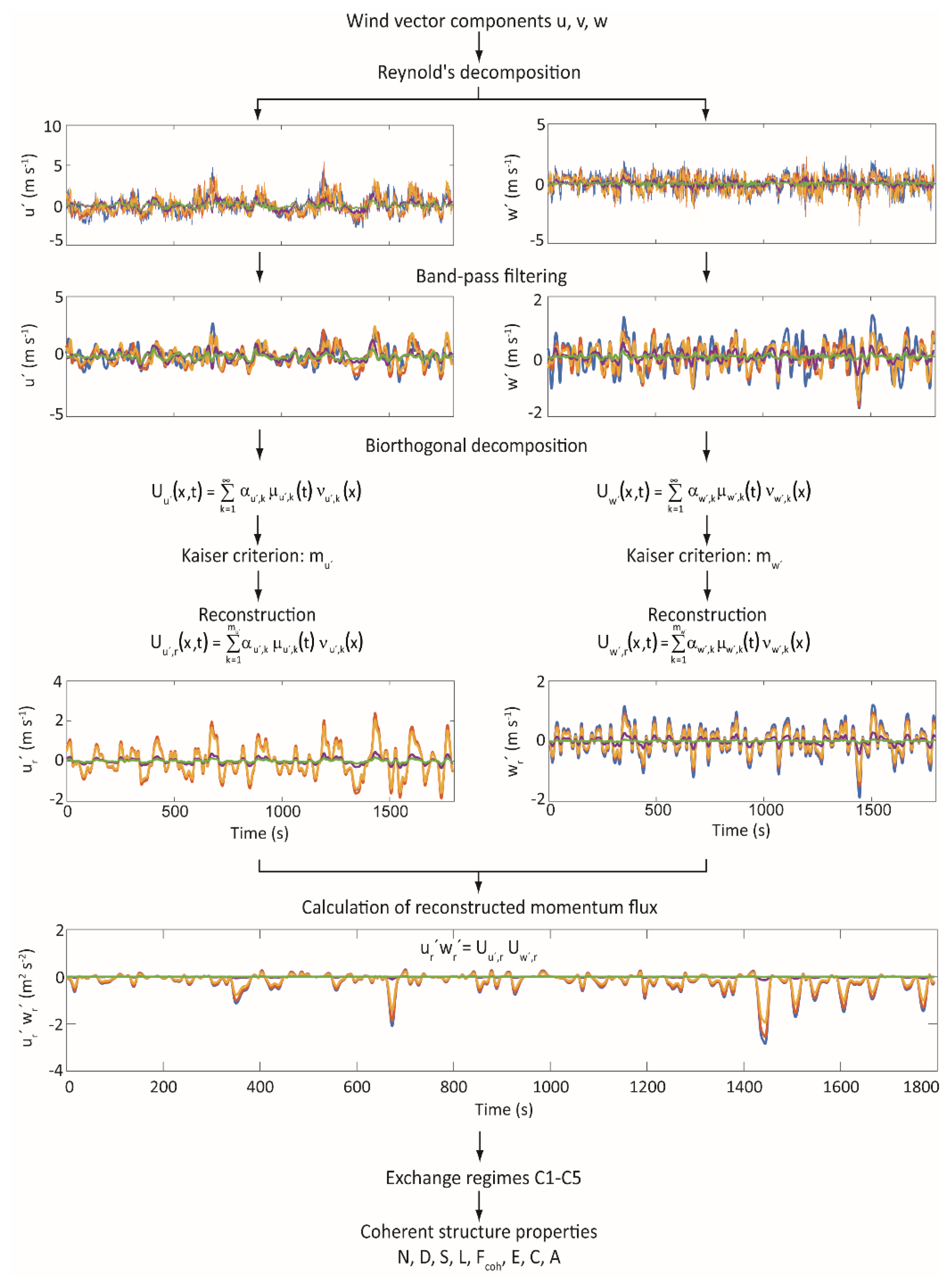
A flowchart (Figure 3) summarizes all steps involved in the data processing.
3. Results and Discussion
3.1. Wavelet Analysis vs. BOD
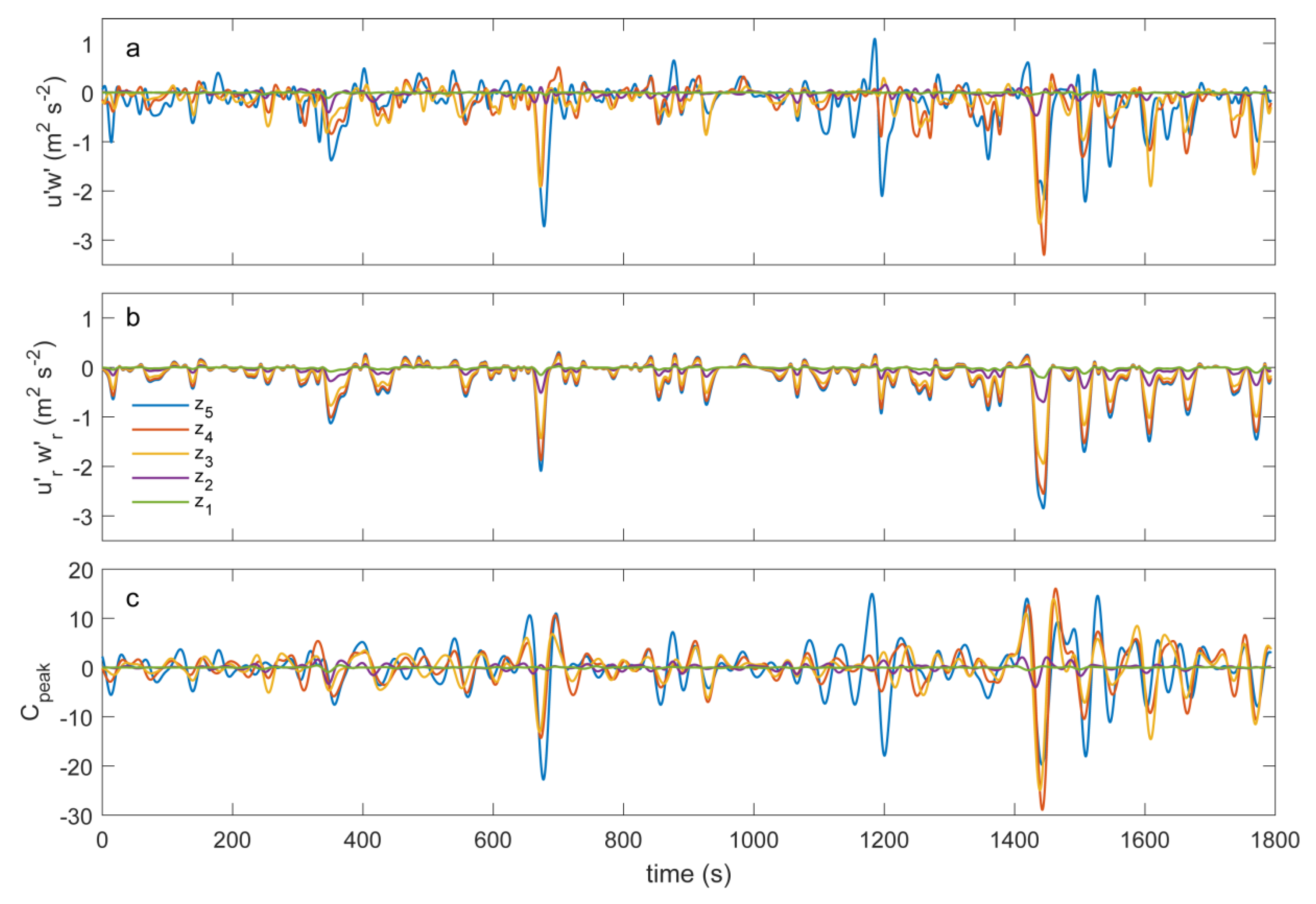
To highlight the differences in the temporal behavior of Cpeak and reconstructed momentum flux , Figure 4 shows a comparison of with and Cpeak over a half-hourly interval (12:30–13:00 CET, 2 August 2014). One useful BOD component explaining 79% of total variance was used to build , and one BOD component explaining 82% of total variance was used to build .
The wavelet analysis is carried out separately at every height. As a consequence, the peak scales speak vary from height to height, which poses a problem when comparing similarities between of adjacent heights. The calculated peak scales for z1–z5 are 91, 95, 104, 106 and 100, corresponding to Fourier-equivalent frequencies (periods) of 0.028 Hz (36.4 s), 0.029 Hz (34.0 s), 0.024 Hz (41.6 s), 0.024 Hz (42.4 s) and 0.025 Hz (40.0 s). On the other hand, the BOD includes z1–z5 simultaneously and produces similar temporal behavior at all measurement heights. Thus, extracts the features in that are common to all heights.
The calculation of the absolute differences between the correlation coefficients obtained from BOD and wavelet analysis over all half-hourly intervals leads to the result that the correlation between , and calculated for any two adjacent heights is 21%, 32% and 46% stronger for BOD than for wavelet analysis (Table 3).
3.2. Exchange Regimes
In the measurement period, C1 covers 42.4% of the analyzed half-hourly intervals. The exchange regime C2 was not detected in the analyzed dataset. The exchange regimes C3–C5, which indicate increasing penetration depth of coherent structures into the below-canopy space, were detected in 23.6%, 15.2% and 18.8% of the half-hourly intervals.
In Table 4, fractions of C1–C5 are summarized as a function of atmospheric stability. From that, it can be inferred that C1 is the dominant exchange regime under stable conditions and transition to stable, covering 92.7% and 64.0% of all cases. Furthermore, it is obvious that with increasing instability, the occurrence of coherent structures penetrating into the canopy clearly increases, as the fractions of C4 and C5 increases. Under forced convection, C4 and C5 dominate, i.e., momentum is transferred from above the canopy into the below-canopy space.
A comparison of the results obtained by BOD with the results reported in previous studies shows general agreement on the proportions of exchange regimes. A study investigated exchange regimes in a spruce forest based on wavelet analysis during a period of five days with [9]. The definition of exchange regimes used in that study was based on the vertical profiles of buoyancy exchange of coherent structures [33]: wave motion (Wa), decoupled canopy (Dc), decoupled sub-canopy (Ds), coupled sub-canopy by sweeps (Cs) and fully-coupled canopy (C).
In terms of coupling between above- and below-canopy airflow, C1 and C2 can be compared to Wa and Dc, C3 to Ds and C4 and C5 to Cs and C. The proportions of exchange regimes reported by [9] are: Wa = 47.3%, Dc = 4.3%, Ds = 17.9%, Cs = 20.1%, C = 10.3%. The results obtained here are: C1 = 42.4%, C2 = 0.0%, C3 = 23.6%, C4 = 15.2%, C5 = 18.8%.
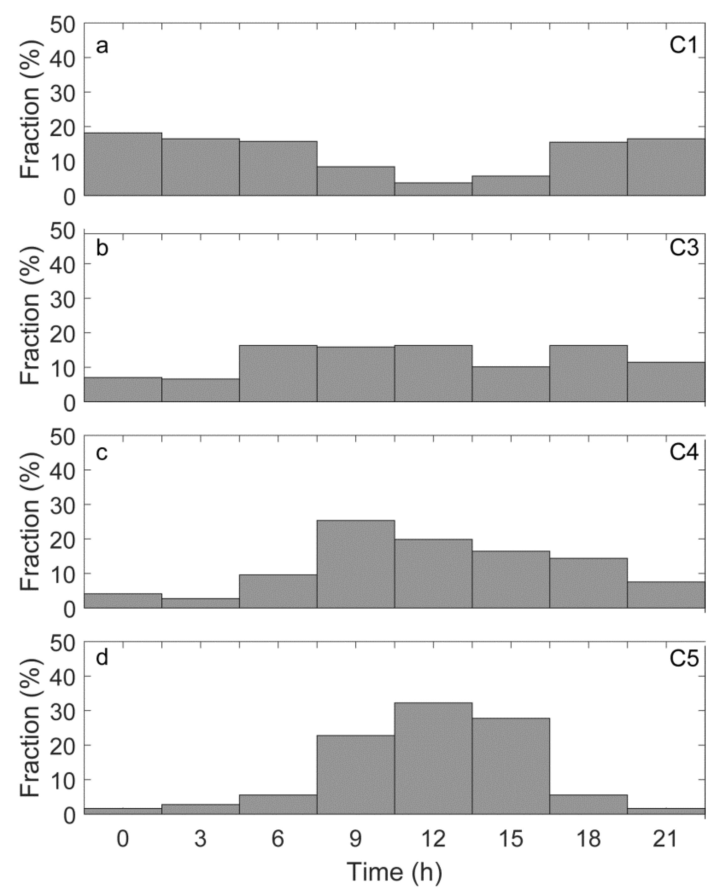
Although a comparison between both studies is not straightforward, because [9] used a classification of exchange regimes based on buoyancy exchange, some common results are found. First, most of the time, there is no coupling between above-canopy air and below-canopy air (Wa + Dc = 51.6%; C1 + C2 = 42.4%). Second, the proportions of exchange regimes associated with a coupling between above- and below-canopy air are in a similar range (Cs + C = 30.4%; C4 + C5 = 34.0%). Furthermore, specific exchange regimes seem to occur at certain times throughout the day (Figure 5). While C1 was observed more often at night, C3–C5 occurred mostly during daytime with C4 occurrence peaking in the morning and C5 occurrence peaking at noon, which is in good agreement with previous findings [33]. With increasing solar radiation, however, stability decreases, which increases the vertical transport. Thus, coupling between air above and below the canopy becomes more likely.
3.3. Detection of Coherent Structures
After applying the BOD, sweeps and ejections were detected separately, and their properties were quantified. In Figure 6, the detection is exemplified for z5. It shows being calculated over an arbitrarily-chosen half-hourly interval (15:00–15:30 CET, 3 June 2014). The reconstruction of is based on two BOD components that explain 85.3% of variance and 81.6% of variance.
Counting sweeps and ejections gives Nmeas = 14 and Nmeas = 16. For each sweep and ejection, its duration, as well as the separation of a subsequent event of the same type is determined for z1–z5 by monitoring the crossings of –H . For example, the first ejection shown in Figure 6 has a duration of Dmeas = 24 s and is followed by a second ejection event after Smeas = 41 s. After determination of Nmeas, Dmeas and Smeas for all 30-min intervals, the values were converted to normalized N, D and S according to Equations (14)–(16).
Table 5 provides comprehensive information on the central tendencies of N for z1–z5 under different exchange regimes. In the entire measurement period varied between seven and 21, and IQR represented 6–27 detected coherent structures, which is comparable to the range of N found in previous studies using wavelet analysis [11,16].
Under fully-coupled conditions, the results of the WRS test demonstrated that at z5, related to sweeps and ejections were significantly larger than below the canopy. Thus, it can be inferred that not all coherent structures detected at z5 contributed to the momentum exchange into the forest. Moreover, for C3–C5, the number of sweeps was significantly larger than the number of ejections at all measurement heights. Therefore, sweeps were the dominating coherent structure type.
3.4. Typical Event Duration and Separation
The median values of D varied between 19.2 s and 26.0 s with IQR spanning from 14.4 s–36.6 s (Table 6). Results from the WRS test showed only significant height-dependent differences under fully-coupled conditions, with D of sweeps and ejections being significantly larger at z1 than at z5. Furthermore, D values of sweeps were significantly shorter than D values of ejections at all heights under C3–C5.
Under all exchange regimes, values varied between 75.7 s and 106.6 s at z1–z5 with IQR spanning from 37.0–201.2 s (Table 7). Results from the WRS test showed no height-specific differences. However, results indicated that for C1–C4, S values for sweeps were shorter than S values for ejections at all measurement heights.
Although there is general agreement between the tendencies obtained for N, D and S in this work and the results obtained in previous studies, a comparison of absolute values is not straightforward because in previous studies: (i) different methods have been applied to detect and study coherent structures for only one or several levels separately; (ii) investigation periods were often much shorter; (iii) the reported results do not refer to the same central tendencies in the data; (iv) a diversity of coherent structure definitions have been used, leading to different definitions of D and S; and (v) a possible bias due to different wind speed at different stability conditions was often not considered.
A study investigated coherent structures during a period of five days with conditions in a spruce forest and found D values in the range 10–30 s [9]. Another study determined a median coherent structure duration of 90–115 s with wavelet analysis and 1.3–1.8 s with quadrant analysis during stable and unstable conditions [7]. Based on visual inspection, D was reported to vary between 24 and 39 s below a deciduous forest canopy and between 20 and 23 s above the canopy during three 30-min intervals with stable, neutral and unstable conditions [2]. Furthermore, based on visual analysis, a mean duration of coherent structures above a pine forest of 33–40 s was determined, with separations of 97–124 s during two 100-min intervals under unstable conditions [49]. Two studies used wavelet analysis to detect coherent structures at a pine forest site during slightly unstable conditions and found characteristic durations and separations around 4 s and 29 s [8,15].
3.5. Further Coherent Structure Characteristics
Median values obtained for L (), Fcoh (), E (), C () and A () for different exchange regimes are summarized in Table 8.
The values spanned between = 43.6 m determined for C1 and = 96.4 m determined for C4. The median values of Fcoh varied between 18.7% and 21.3% below the canopy and between 29.8% and 39.4% at and above the canopy. Median transport efficiency included values between = 0.6 and = 0.7 below the canopy and between = 1.1 and = 1.3 at the canopy height and above the canopy. Median total time cover of coherent structures varied between = 27.5% and = 29.2%.
Results from the WRS test showed that the values of for C4 and C5 were significantly larger than the values calculated for C1 and C3, suggesting that only large coherent structures reached the subcanopy space. For C3–C5, the values for and at z5 were significantly smaller than the values at canopy height, but significantly larger than the values below the canopy. This suggests that momentum flux was enhanced through shear-generated momentum flux at canopy height, but weakened through dissipation in the subcanopy space. Height-specific differences in indicate that coherent structures transferred momentum efficiently above the canopy. However, below the canopy, the transport efficiency of momentum flux through coherent structures was weakened.
This is also visible in the calculated values for . The amplitude of coherent structures involved in momentum transport from z5–z1 was strongly attenuated below the canopy.
Median values obtained for L, Fcoh, E and C related to different stability conditions are summarized in Table 9.
Results from the WRS test indicated a dependence of on atmospheric stability. For all heights, was significantly larger during near-neutral conditions and forced convection than under stable conditions and transition to stable. Thus, in agreement with findings from a previous study [11], an increase of with increasing instability was found. Under stable stratification, the formation of large coherent eddies was inhibited, which led to the dominance of eddies with smaller sizes.
Although the magnitude of Fcoh largely depends on the method of analysis [33], the results above the canopy obtained in this study agree well with the results from previous studies: One study [7] reported median values of Fcoh between 40% and 48% by analyzing coherent structures in a deciduous forest at canopy height. Another study [11] found mean values of Fcoh between 38% and 51% at 10 m and 30 m above a mixed surface. Over a pine forest, Fcoh of 92.7% ± 3.2% was reported [49]. In an urban area, a study [39] found that Fcoh ranged between 41% and 107% at z/h = 1.5 under unstable conditions. Values of Fcoh between 55% and 95% were derived in a walnut orchard during different stability conditions from quadrant analysis using a hole parameter of H = 3 [6].
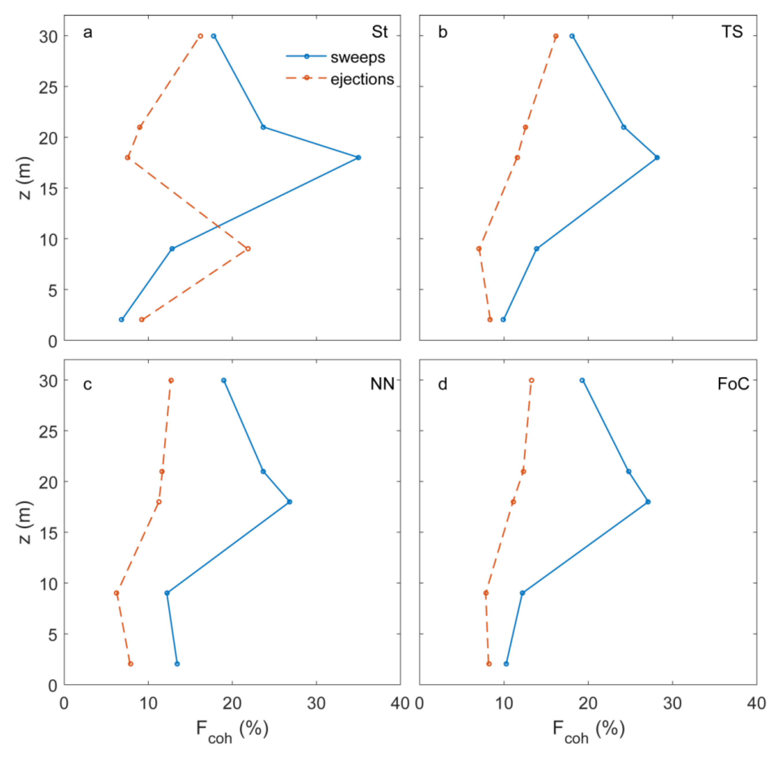
Results from the analysis of the contribution of sweeps and ejections to Fcoh under different atmospheric stabilities are shown in Figure 7. Values for Fcoh,sw peaked at canopy height and decreased with height above the canopy, whereas Fcoh,ej still increased above the canopy. This behavior was also observed in a previous study [33]. Increasing Fcoh,ej above the canopy indicates the transition from a flow dominated by shear-driven coherent structures to a flow associated with rough-wall boundary layers [6].
The authors of a previous study [3] concluded from their results that the magnitude of sweeps are larger than the magnitude of ejections under unstable conditions and that the strength of both decreases with increasing stability. The larger magnitude of sweeps was also observed in this study. However, a decrease in the strength of sweeps and ejections with increasing stability was not found.
An investigation [49] of coherent structures above a pine forest under unstable conditions (–1 < ζ < 0) came to the conclusion that the proportions of sweeps are higher compared to ejections at canopy height and that the importance of ejections increases with increasing height from the canopy top. Numerous studies [1,2,6,33,45] found similar results.
An increase of ejections with height was also observed in this study. Furthermore, the authors of some studies [2,50] concluded from their results that sweeps and ejections contribute most to the overall transport in the canopy and that the sweeps-related contribution dominates. This statement can be confirmed from the findings obtained in this study.
It was also reported that the contribution of ejections increased in the below-canopy space and that the contributions of sweeps and ejections become equal further down to the ground [33]. An increase of ejections with decreasing height was not found in this work, whereas the contributions of sweeps and ejections did approach each other near the ground. During stable conditions, ejections dominated in the sub-canopy space.
The values determined above the canopy were similar to the values (1.05–1.66) found by previous studies [11,16]. Under different atmospheric stabilities, varied between 24.4% and 30.8%. Results from the WRS test showed significant height-specific differences, as well as stability-specific differences. During transition to stable, at z5 was significantly larger than at z4 and z3, but also significantly smaller than below the canopy. Under stable conditions, at z5 was larger than directly at z4 and z3. Since Fcoh always peaked at the canopy top, this result indicates the occurrence of strong, but short sweeps and ejections during transition to stable and stable conditions. Overall, the values are in good agreement with previous studies ([11]: = 25%–45%; [49]: = 28%–38%).
4. Conclusions
The contribution of synchronous coherent structures to the exchange of momentum was investigated in a planted Scots pine forest. Coherent structures are known to substantially contribute to the transfer of momentum in vegetation canopies. To quantify their contribution to the total momentum transfer, single-level detection methods have been applied in previous studies. The disadvantage of these methods, however, is that detection results differ between the investigated levels. Therefore, the BOD was presented as a tool for the synchronous detection of coherent structures in the vertical momentum exchange between the Scots pine forest and the atmosphere. The BOD simultaneously treats the momentum flux measured at multiple levels, which is a major advantage over commonly-applied single-level methods, such as wavelet analysis. Furthermore, the BOD allowed for the analysis of coupling between above- and below-canopy momentum fluxes.
It was found that fully-coupled turbulent momentum exchange over all measurement heights occurred during 19% of all analyzed half-hourly datasets, mostly during daytime. At night, under stable conditions, the subcanopy layer was most frequently decoupled from the above-canopy layer. From the synchronous coherent structures extracted from the momentum flux, sweep and ejection characteristics, such as the number of occurrences, duration and separation, were quantified. The median values for the number of occurrence per 30-min interval, duration and separation were 7–21, 14.4–36.6 s and 75.7–106.6 s. The contribution of the detected sweeps and ejections to total momentum flux, their transport efficiency, as well as their time cover were 16.1%–40.8%, 0.6–1.5 and 24.4%–30.8%.
Results suggest that momentum transfer through synchronous coherent structures is very efficient above the forest canopy, but attenuated in the below-canopy space, which might result from the generation of small-scale turbulent structures by the Scots pine trees, which induces a short-circuiting of momentum transfer. This implies that canopy characteristics, such as density and vertical distribution of biomass, have considerable effects on the characteristics of coherent structures.
Although there is general agreement between the majority of the presented results and results obtained in previous studies that used single-level analysis methods, this work is considered as a first case study for coherent structure detection using the BOD. Therefore, there is potential for improvement of the methodology and the reduction of uncertainty associated with the choice of the required thresholds. Further comparisons with wavelet-based detection of coherent structures will show whether the proposed methodology is suitable not only for momentum exchange, but also for the exchange of scalar quantities, such as temperature or CO2.
Acknowledgments
This research is funded by the German Research Foundation (SCHI 868/3-1).
Author Contributions
Manuel Mohr designed the research, performed the data analysis, and wrote the manuscript. Dirk Schindler developed the research idea and co-wrote the manuscript.
Conflicts of Interest
The authors declare no conflict of interest.
References
- Finnigan, J. Turbulence in plant canopies. Annu. Rev. Fluid Mech. 2000, 32, 519–571. [Google Scholar] [CrossRef]
- Gao, W.; Shaw, R.H.; Paw, K.T.U. Observation of organized structure in turbulent flow within and above a forest canopy. Bound. Layer Meteorol. 1989, 47, 349–377. [Google Scholar] [CrossRef]
- Gao, W.; Shaw, R.H.; Paw, K.T.U. Conditional analysis of temperature and humidity microfronts and ejection/sweep motions within and above deciduous forest. Bound. Layer Meteorol. 1992, 59, 35–57. [Google Scholar] [CrossRef]
- Wilczak, J.M. Large-scale eddies in the unstably stratified atmospheric surface layer. Part I: Velocity and temperature structures. J. Atmos. Sci. 1984, 41, 3537–3550. [Google Scholar] [CrossRef]
- Finnigan, J.J. Turbulence in weaving wheat; II: Structure of momentum transfer. Bound. Layer Meteorol. 1979, 16, 213–236. [Google Scholar]
- Dupont, S.; Patton, E.G. Momentum and scalar transport within a vegetation canopy following atmospheric stability and seasonal canopy changes. Atmos. Chem. Phys. 2012, 12, 5913–5935. [Google Scholar] [CrossRef]
- Steiner, A.L.; Pressley, S.N.; Botros, A.; Jones, E.; Chung, S.H.; Edburg, S.L. Analysis of coherent structures and atmosphere-canopy coupling strength during the CABINEX field campaign. Atmos. Chem. Phys. 2011, 11, 11921–11936. [Google Scholar] [CrossRef]
- Collineau, S.; Brunet, Y. Detection of turbulent coherent motions in a forest canopy—Part I: Wavelet Analysis. Bound. Layer Meteorol. 1993, 65, 357–379. [Google Scholar]
- Serafimovich, A.; Thomas, C.; Foken, T. Vertical and horizontal transport of energy and matter by coherent motions in a tall spruce canopy. Bound. Layer Meteorol. 2011, 140, 429–451. [Google Scholar] [CrossRef]
- Krusche, N.; de Oliveira, A.P. Characterization of coherent structures in the atmospheric boundary-layer. Bound. Layer Meteorol. 2004, 110, 191–211. [Google Scholar] [CrossRef]
- Barthlott, C.; Drobinski, P.; Fesquet, C.; Dubos, T.; Pietras, C. Long-term study of coherent structures in the atmospheric surface layer. Bound. Layer Meteorol. 2007, 125, 1–24. [Google Scholar] [CrossRef]
- Thomas, C.; Foken, T. Detection of long-term coherent exchange over spruce forest using wavelet analysis. Theor. Appl. Climatol. 2005, 80, 91–104. [Google Scholar] [CrossRef]
- Lu, C.H.; Fitzjarrald, D.R. Seasonal and diurnal variations of coherent structures over a deciduous forest. Bound. Layer Meteorol. 1994, 69, 43–69. [Google Scholar] [CrossRef]
- Chen, J.; Hu, F. Coherent structures detected in atmospheric boundary-layer turbulence using wavelet transforms at Huaihe River basin, China. Bound. Layer Meteorol. 2003, 107, 429–444. [Google Scholar] [CrossRef]
- Collineau, S.; Brunet, Y. Detection of turbulent coherent motions in a forest canopy—Part II: Time-scales and conditional averages. Bound. Layer Meteorol. 1993, 66, 49–73. [Google Scholar] [CrossRef]
- Starkenburg, D.; Fochesatto, G.J.; Prakash, A.; Cristobal, J.; Gens, R.; Kane, D.L. The role of coherent flow structures in the sensible heat fluxes of an Alaskan boreal forest. J. Geophys. Res. Atmos. 2013, 118, 8140–8155. [Google Scholar] [CrossRef]
- Raupach, M.R.; Antonia, R.A.; Rajagopalan, S. Rough-wall turbulent boundary layers. Appl. Mech. Rev. 1991, 44, 1–25. [Google Scholar] [CrossRef]
- Sörgel, M.; Trebs, I.; Serafimovich, A.; Moravek, A.; Held, A.; Zetzsch, C. Simultaneous HONO measurements in and above a forest canopy: Influence of turbulent exchange on mixing ratio differences. Atmos. Chem. Phys. 2011, 11, 841–855. [Google Scholar] [CrossRef]
- Foken, T.; Meixner, F.X.; Falge, E.; Zetzsch, C.; Serafimovich, A.; Bargsten, A.; Behrendt, T.; Biermann, T.; Breuninger, C.; Dix, S.; et al. Coupling processes and exchange of energy and reactive and non-reactive trace gases at a forest site—Results of the EGER experiment. Atmos. Chem. Phys. 2012, 12, 1923–1950. [Google Scholar] [CrossRef] [Green Version]
- Baldocchi, D.D.; Falge, E.; Gu, L.; Olson, R.; Hollinger, D.; Running, S.; Anthoni, P.; Bernhofer, C.; Davis, K.; Evans, R.; et al. FLUXNET: A new tool to study the temporal and spatial variability of ecosystem-scale carbon dioxide, water vapour and energy flux densities. Bull. Am. Meteorol. Soc. 2001, 82, 2415–2434. [Google Scholar] [CrossRef]
- Schindler, D.; Vogt, R.; Fugmann, H.; Rodriguez, M.; Schönborn, J.; Mayer, H. Vibration behavior of plantation-grown Scots pine trees in response to wind excitation. Agric. For. Meteorol. 2010, 150, 984–993. [Google Scholar] [CrossRef]
- Schindler, D.; Fugmann, H.; Schönborn, J.; Mayer, H. Coherent response of a group of plantation-grown Scots pine trees to wind loading. Eur. J. For. Res. 2012, 131, 191–202. [Google Scholar] [CrossRef]
- Aubry, N.; Guyonnet, R.; Lima, R. Spatiotemporal analysis of complex signals: Theory and applications. J. Stat. Phys. 1991, 64, 683–739. [Google Scholar] [CrossRef]
- Py, C.; de Langre, E.; Moulia, B.; Hémon, P. Measurement of wind-induced motion of crop canopies from digital video images. Agric. For. Meteorol. 2005, 130, 223–236. [Google Scholar] [CrossRef]
- Py, C.; de Langre, E.; Moulia, B. A frequency lock-in mechanism in the interaction between wind and crop canopies. J. Fluid Mech. 2006, 568, 425–449. [Google Scholar] [CrossRef]
- Kaimal, J.C.; Finnigan, J.J. Atmospheric Boundary Layer Flows: Their Structure and Measurement; Oxford University Press: New York, NY, USA, 1994. [Google Scholar]
- Rebmann, C.; Kolle, O.; Heinesch, B.; Queck, R.; Ibrom, A.; Aubinet, M. Data acquisition and flux calculations. In Eddy Covariance; Aubinet, M., Vesala, T., Papale, D., Eds.; Springer: Dordrecht, the Netherlands, 2012; pp. 59–83. [Google Scholar]
- Obukhov, A.M. Turbulence in an atmosphere with a non-uniform temperature. Tr. Inst. Teor. Geofiz. Akad. Nauk. SSSR 1946, 1, 95–115. [Google Scholar] [CrossRef]
- Stull, R.B. An Introduction to Boundary Layer Meteorology; Kluwer Academic Publishers: Berlin, Germany, 1988; p. 666. [Google Scholar]
- Dupont, S.; Patton, E.G. Influence of stability and seasonal canopy changes on micrometeorology within and above an orchard canopy: The CHATS experiment. Agric. For. Meteorol. 2012, 157, 11–29. [Google Scholar] [CrossRef]
- Van Gorsel, E.; Harman, I.N.; Finnigan, J.J.; Leuning, R. Decoupling of air flow above and in plant canopies and gravity waves affect micrometeorological estimates of net scalar exchange. Agric. For. Meteorol. 2011, 151, 927–933. [Google Scholar] [CrossRef]
- Thomas, C.; Foken, T. Organised motion in a tall spruce canopy: Temporal scales, structure spacing and terrain effects. Bound. Layer Meteorol. 2007, 122, 123–147. [Google Scholar] [CrossRef]
- Thomas, C.; Foken, T. Flux contribution of coherent structures and its implications for the exchange of energy and matter in a tall spruce canopy. Bound. Layer Meteorol. 2007, 123, 317–337. [Google Scholar] [CrossRef]
- Gao, W.; Li, B.L. Wavelet analysis of coherent structures at the atmosphere-forest interface. J. Appl. Meteorol. 1993, 32, 1717–1725. [Google Scholar] [CrossRef]
- Torrence, C.; Compo, G.P. A practical guide to wavelet analysis. Bull. Am. Meteorol. Soc. 1998, 79, 61–78. [Google Scholar] [CrossRef]
- Brunet, Y.; Irvine, M.R. The control of coherent eddies in vegetation canopies: Streamwise structure spacing, canopy shear scale and atmospheric stability. Bound. Layer Meteorol. 2000, 94, 139–163. [Google Scholar] [CrossRef]
- Thomas, C.; Mayer, J.-C.; Meixner, F.X.; Foken, T. Analysis of low-frequency turbulence above tall vegetation using a Doppler sodar. Bound. Layer Meteorol. 2006, 119, 563–587. [Google Scholar] [CrossRef]
- Mahrt, L.; Howell, J.F. The influence of coherent structures and microfronts on scaling laws using global and local transforms. J. Fluid Mech. 1994, 260, 247–270. [Google Scholar] [CrossRef]
- Feigenwinter, C.; Vogt, R. Detection and analysis of coherent structures in urban turbulence. Theor. Appl. Climatol. 2005, 81, 219–230. [Google Scholar] [CrossRef]
- Abry, P. Ondelettes et Turbulence: Multirésolutions, Algorithmes de Décomposition, Invariance d’échelles; Diderot Editeur: Paris, France, 1997. [Google Scholar]
- Hémon, P.; Santi, F. Applications of biorthogonal decompositions in fluid-structure interactions. J. Fluid Struct. 2003, 17, 1123–1143. [Google Scholar] [CrossRef]
- Cattell, R.B. The scree test for the number of factors. Multivar. Behav. Res. 1966, 1, 245–276. [Google Scholar] [CrossRef] [PubMed]
- Kaiser, H.F. The application of electronic computers to factor analysis. Educ. Psychol. Meas. 1960, 20, 141–151. [Google Scholar] [CrossRef]
- Poggi, D.; Porporato, A.; Ridolfi, L.; Albertson, J.D.; Katul, G.G. The effect of vegetation density on canopy sub-layer turbulence. Bound. Layer Meteorol. 2004, 111, 565–587. [Google Scholar] [CrossRef]
- Shaw, R.H.; Tavangar, J.; Ward, D.P. Structure of the Reynolds stress in a canopy layer. J. Clim. Appl. Meteorol. 1983, 22, 1922–1931. [Google Scholar] [CrossRef]
- Lu, S.S.; Willmarth, W.W. Measurement of the structure of the Reynolds stress in a turbulent boundary layer. J. Fluid Mech. 1973, 60, 481–511. [Google Scholar] [CrossRef]
- Mann, H.B.; Whitney, D.R. On a test of whether one of two random variables is stochastically larger than the other. Ann. Math. Stat. 1947, 18, 50–60. [Google Scholar] [CrossRef]
- Taylor, G.I. The spectrum of turbulence. Proc. R. Soc. Lon. Ser. A 1938, 164, 476–490. [Google Scholar] [CrossRef]
- Bergström, H.; Högström, U. Turbulent exchange above a pine forest II: Organized structures. Bound. Layer Meteorol. 1989, 49, 231–263. [Google Scholar] [CrossRef]
- Raupach, M.R.; Finnigan, J.J.; Brunet, Y. Coherent eddies and turbulence in vegetation canopies: The mixing-layer analogy. Bound. Layer Meteorol. 1996, 78, 351–382. [Google Scholar] [CrossRef]
Figure 1.
(a) Normalized vertical profile of plant area density (PAD) and (b) wind rose at z3 at the measurement site.
Figure 1.
(a) Normalized vertical profile of plant area density (PAD) and (b) wind rose at z3 at the measurement site.
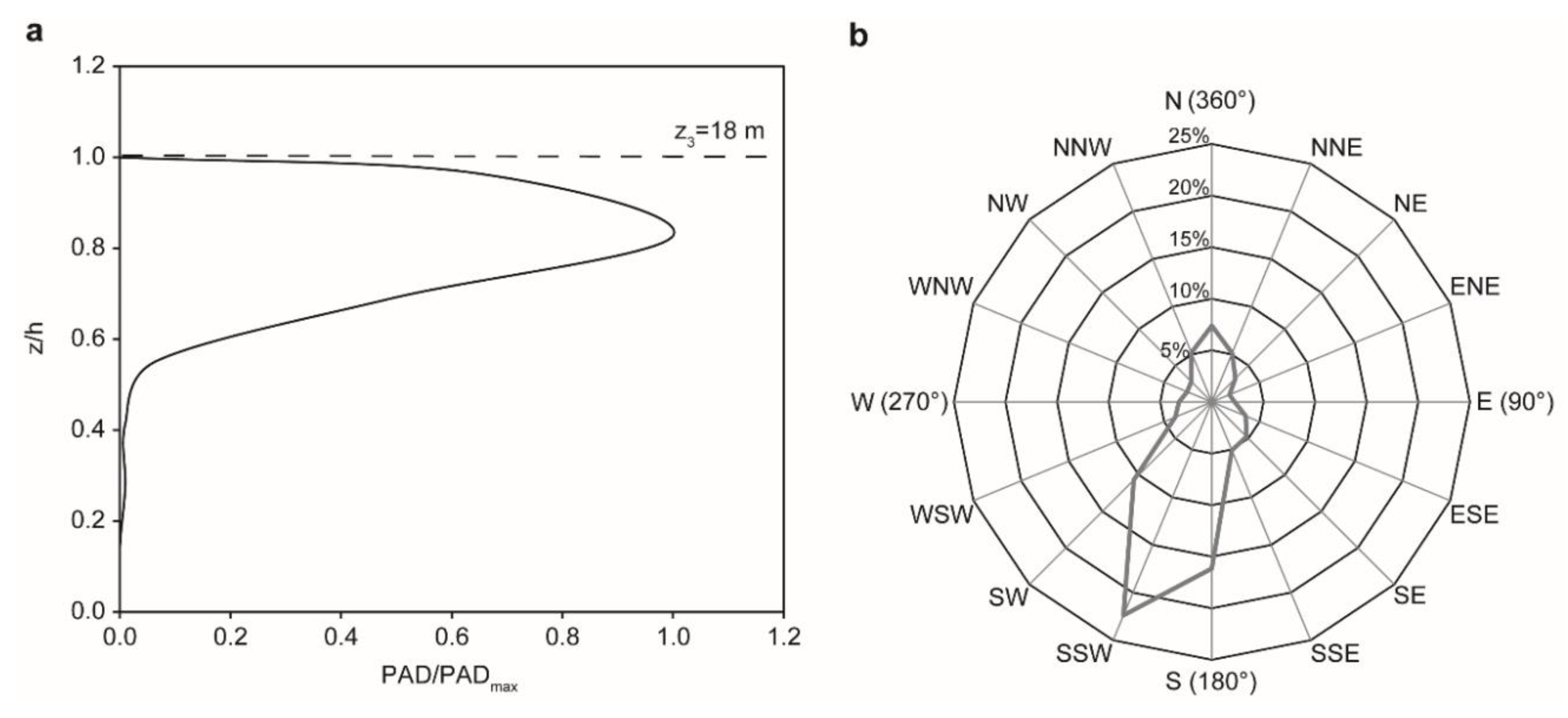
Figure 2.
Scree plot of u’ for a half-hourly interval (11:30–12:00 CET, 4 June 2014): eigenvalues of the five biorthogonal decomposition (BOD) terms (red) and the mean value of all eigenvalues (green).
Figure 2.
Scree plot of u’ for a half-hourly interval (11:30–12:00 CET, 4 June 2014): eigenvalues of the five biorthogonal decomposition (BOD) terms (red) and the mean value of all eigenvalues (green).

Figure 3.
Flowchart summarizing all steps involved in the data processing.

Figure 4.
Half-hourly time series (12:30–13:00 CET, 2 August 2014): of (a) u’w’; (b) of ur’wr’. The colors indicate momentum flux at z1–z5. Variance explained by ur’ using one BOD component is 79%; variance explained by wr’ using one BOD component is 82%. To improve visibility, ur’wr’ calculated at z2 and z1 was enhanced five- and 20-fold. For comparison; (c) shows the wavelet coefficients Cpeak related to z1–z5.

Figure 5.
Diurnal patterns of C1, C3, C4 and C5 fractions.

Figure 6.
Identification and classification of sweeps and ejections at z5 using local ur’wr’ (15:00–15:30 CET, 3 June 2014).
Figure 6.
Identification and classification of sweeps and ejections at z5 using local ur’wr’ (15:00–15:30 CET, 3 June 2014).

Figure 7.
Fcoh of sweeps (Fcoh,sw) and ejections (Fcoh,ej) at z1–z5 under different stability conditions (St, TS, NN, FoC).
Figure 7.
Fcoh of sweeps (Fcoh,sw) and ejections (Fcoh,ej) at z1–z5 under different stability conditions (St, TS, NN, FoC).


| Stability Class | ζ3 |
|---|---|
| Very stable (VS) | >1 |
| Stable (St) | 0.6 to 1 |
| Transition to stable (TS) | 0.02 to 0.6 |
| Near-neutral (NN) | –0.03 to 0.02 |
| Forced convection (FoC) | –0.8 to –0.03 |
| Free convection (FrC) | <–0.8 |
Table 2.
Combinations of momentum flux direction at z1–z5 with corresponding definitions of exchange regimes C1–C5. The proportions of C1–C5 occurrence are given in the last row.
| Exchange Regime | C1 | C2 | C3 | C4 | C5 | |||||||||||
|---|---|---|---|---|---|---|---|---|---|---|---|---|---|---|---|---|
| Combination | 1 | 2 | 3 | 4 | 5 | 6 | 7 | 8 | 9 | 10 | 11 | 12 | 13 | 14 | 15 | 16 |
| z5 | ↓ | ↓ | ↓ | ↓ | ↓ | ↓ | ↓ | ↓ | ↓ | ↓ | ↓ | ↓ | ↓ | ↓ | ↓ | ↓ |
| z4 | ↑ | ↑ | ↑ | ↑ | ↑ | ↑ | ↑ | ↑ | ↓ | ↓ | ↓ | ↓ | ↓ | ↓ | ↓ | ↓ |
| z3 | ↑ | ↑ | ↑ | ↑ | ↓ | ↓ | ↓ | ↓ | ↑ | ↑ | ↑ | ↑ | ↓ | ↓ | ↓ | ↓ |
| z2 | ↑ | ↑ | ↓ | ↓ | ↑ | ↑ | ↓ | ↓ | ↑ | ↑ | ↓ | ↓ | ↑ | ↑ | ↓ | ↓ |
| z1 | ↑ | ↓ | ↑ | ↓ | ↑ | ↓ | ↑ | ↓ | ↑ | ↓ | ↑ | ↓ | ↑ | ↓ | ↑ | ↓ |
| Fraction (%) | 3.0 | 4.2 | 9.3 | 25.6 | 0.0 | 0.3 | 0.0 | 0.0 | 0.0 | 0.0 | 0.0 | 0.0 | 22.7 | 0.9 | 15.2 | 18.8 |
Table 3.
First quartile (Q1), median and third quartile (Q3) of the difference between the correlation coefficients (R) calculated for adjacent heights (z1–z5) obtained from the reconstructed time series using BOD (ur’, wr’, ur’wr’) and peak wavelet coefficients (Cpeak,u’, Cpeak,w’, Cpeak,u’w’).
| Quantity | z1–z2 | z2–z3 | z3–z4 | z4–z5 | all | |
|---|---|---|---|---|---|---|
| Q1 | 0.13 | 0.67 | 0.07 | 0.08 | 0.11 | |
| median | 0.17 | 0.84 | 0.10 | 0.24 | 0.21 | |
| Q3 | 0.24 | 0.93 | 0.14 | 0.36 | 0.53 | |
| Q1 | 0.38 | 0.31 | 0.08 | 0.05 | 0.13 | |
| median | 0.45 | 0.37 | 0.11 | 0.27 | 0.32 | |
| Q3 | 0.56 | 0.45 | 0.15 | 0.35 | 0.43 | |
| Q1 | 0.44 | 0.67 | 0.14 | 0.15 | 0.21 | |
| median | 0.55 | 0.81 | 0.19 | 0.39 | 0.46 | |
| Q3 | 0.67 | 0.90 | 0.25 | 0.52 | 0.68 |
| Stability | C1 | C2 | C3 | C4 | C5 |
|---|---|---|---|---|---|
| Stable (St) | 92.7 | 0.0 | 5.5 | 0.0 | 1.8 |
| Transition to stable (TS) | 64.0 | 0.0 | 24.8 | 8.1 | 3.1 |
| Near-neutral (NN) | 16.7 | 0.0 | 40.3 | 30.6 | 12.5 |
| Forced convection (FoC) | 18.2 | 0.0 | 22.0 | 21.8 | 38.0 |
Table 5.
First quartile, median and third quartile of N of sweeps and ejections detected during half-hourly intervals under different exchange regimes (C1, C3, C4, C5).
| Sweeps | Ejections | |||||||
|---|---|---|---|---|---|---|---|---|
| Height | C1 | C3 | C4 | C5 | C1 | C3 | C4 | C5 |
| z1 | 7, | 6, | ||||||
| 8, | 7, | |||||||
| 11 | 9 | |||||||
| z2 | 8, | 8, | 6, | 6, | ||||
| 11, | 9, | 8, | 8, | |||||
| 14 | 12 | 10 | 10 | |||||
| z3 | 11, | 9, | 9, | 8, | 7, | 8, | ||
| 13, | 12, | 12, | 10, | 8, | 10, | |||
| 15 | 15 | 14 | 12 | 11 | 12 | |||
| z4 | 11, | 9, | 9, | 8, | 7, | 8, | ||
| 13, | 12, | 12, | 10, | 8, | 10, | |||
| 15 | 15 | 15 | 12 | 11 | 13 | |||
| z5 | 16, | 11, | 9, | 9, | 16, | 8, | 7, | 8, |
| 21, | 13, | 12, | 12, | 20, | 10, | 8, | 10, | |
| 27 | 15 | 15 | 15 | 26 | 12 | 11 | 13 | |
Table 6.
First quartile, median and third quartile of D (in s) of sweeps and ejections detected during half-hourly intervals under different exchange regimes (C1, C3, C4, C5).
| Sweeps | Ejections | |||||||
|---|---|---|---|---|---|---|---|---|
| Height | C1 | C3 | C4 | C5 | C1 | C3 | C4 | C5 |
| z1 | 18.3, | 19.1, | ||||||
| 24.1, | 26.0, | |||||||
| 33.2 | 36.6 | |||||||
| z2 | 17.5, | 18.2, | 18.6, | 18.9, | ||||
| 22.5, | 23.8, | 24.9, | 25.8, | |||||
| 31.0 | 32.9 | 34.3 | 35.9 | |||||
| z3 | 17.4, | 17.4, | 17.8, | 18.1, | 18.4, | 18.6, | ||
| 22.0, | 22.3, | 23.4, | 23.7, | 24.7, | 25.1, | |||
| 29.9 | 30.8 | 32.4 | 32.8 | 34.0 | 35.0 | |||
| z4 | 17.4, | 17.4, | 17.8, | 18.2, | 18.5, | 18.6, | ||
| 22.0, | 22.4, | 23.3, | 23.7, | 24.5, | 25.0, | |||
| 29.9 | 30.7 | 32.4 | 32.7 | 34.0 | 34.9 | |||
| z5 | 14.4, | 17.4, | 17.4, | 17.8, | 14.7, | 18.1, | 18.5, | 18.5, |
| 19.2, | 22.0, | 22.3, | 23.3, | 19.6, | 23.8, | 24.4, | 25.0, | |
| 26.7 | 30.0 | 30.7 | 32.3 | 27.2 | 32.8 | 33.9 | 34.8 | |
Table 7.
First quartile, median and third quartile of S (in s) of sweeps and ejections detected during half-hourly intervals under different exchange regimes (C1, C3, C4, C5).
| Sweeps | Ejections | |||||||
|---|---|---|---|---|---|---|---|---|
| Height | C1 | C3 | C4 | C5 | C1 | C3 | C4 | C5 |
| z1 | 51.1, | 51.8, | ||||||
| 106.6, | 103.3, | |||||||
| 186.2 | 188.2 | |||||||
| z2 | 48.2, | 51.1, | 51.1, | 51.5, | ||||
| 95.7, | 106.2, | 103.8, | 101.0, | |||||
| 165.3 | 184.8 | 201.2 | 186.6 | |||||
| z3 | 47.2, | 48.1, | 49.3, | 48.7, | 50.7, | 50.5, | ||
| 94.7, | 95.0, | 105.1, | 100.8, | 102.7, | 97.7, | |||
| 169.1 | 164.4 | 180.0 | 184.7 | 199.7 | 182.4 | |||
| z4 | 47.2, | 48.0, | 49.1, | 49.3, | 50.7, | 50.5, | ||
| 94.9, | 94.9, | 104.7, | 100.5, | 102.7, | 96.9, | |||
| 169.1 | 164.4 | 180.0 | 185.0 | 199.1 | 182.4 | |||
| z5 | 37.0, | 47.2, | 47.9, | 48.7, | 51.8, | 49.4, | 50.7, | 50.1, |
| 75.7, | 95.3, | 94.8, | 104.7, | 78.4, | 100.6, | 102.7, | 96.9, | |
| 132.6 | 169.4 | 164.0 | 180.0 | 188.2 | 185.0 | 198.6 | 182.1 | |
| Variable | Height | C1 | C3 | C4 | C5 |
|---|---|---|---|---|---|
| z1 | 91.4 | ||||
| z2 | 96.4 | 91.4 | |||
| z3 | 82.8 | 96.4 | 91.4 | ||
| z4 | 82.9 | 96.4 | 91.4 | ||
| z5 | 43.6 | 82.9 | 96.4 | 91.4 | |
| z1 | 18.7 | ||||
| z2 | 21.3 | 20.8 | |||
| z3 | 39.4 | 38.8 | 38.8 | ||
| z4 | 37.2 | 37.5 | 36.9 | ||
| z5 | 37.3 | 29.8 | 31.0 | 31.3 | |
| z1 | 0.6 | ||||
| z2 | 0.7 | 0.7 | |||
| z3 | 1.3 | 1.2 | 1.2 | ||
| z4 | 1.3 | 1.2 | 1.2 | ||
| z5 | 1.2 | 1.1 | 1.1 | 1.1 | |
| z1 | 29.2 | ||||
| z2 | 28.6 | 29.2 | |||
| z3 | 27.5 | 28.6 | 29.2 | ||
| z4 | 27.5 | 28.6 | 29.2 | ||
| z5 | 31.5 | 27.5 | 28.6 | 29.2 | |
| z1 | 0.1 | ||||
| z2 | 0.5 | 1.8 | |||
| z3 | 72.9 | 71.1 | 69.9 | ||
| z4 | 93.9 | 93.6 | 90.2 | ||
| z5 | 100 | 100 | 100 | 100 |
| Variable | Height | St | TS | NN | FoC |
|---|---|---|---|---|---|
| z1 | 26.4 | 90.2 | 109.5 | 91.4 | |
| z2 | 26.4 | 82.7 | 109.1 | 94.3 | |
| z3 | 28.2 | 81.6 | 99.4 | 91.8 | |
| z4 | 28.2 | 81.7 | 99.4 | 91.8 | |
| z5 | 31.7 | 58.5 | 91.9 | 85.4 | |
| z1 | 16.1 | 18.8 | 22.3 | 18.5 | |
| z2 | 34.6 | 21.6 | 18.6 | 21.1 | |
| z3 | 40.8 | 39.7 | 38.4 | 38.8 | |
| z4 | 39.1 | 37.1 | 36.1 | 37.5 | |
| z5 | 34.7 | 34.7 | 30.8 | 32.3 | |
| z1 | 0.6 | 0.7 | 0.8 | 0.6 | |
| z2 | 1.2 | 0.7 | 0.6 | 0.7 | |
| z3 | 1.2 | 1.3 | 1.3 | 1.2 | |
| z4 | 1.5 | 1.3 | 1.2 | 1.2 | |
| z5 | 1.1 | 1.1 | 1.1 | 1.1 | |
| z1 | 28.0 | 27.8 | 27.8 | 29.3 | |
| z2 | 28.0 | 27.8 | 27.8 | 29.2 | |
| z3 | 24.4 | 27.8 | 28.1 | 28.8 | |
| z4 | 24.4 | 27.8 | 28.1 | 28.8 | |
| z5 | 30.8 | 30.0 | 28.6 | 29.3 |
© 2016 by the authors; licensee MDPI, Basel, Switzerland. This article is an open access article distributed under the terms and conditions of the Creative Commons Attribution (CC-BY) license (http://creativecommons.org/licenses/by/4.0/).
Share and Cite
MDPI and ACS Style
Mohr, M.; Schindler, D. Coherent Momentum Exchange above and within a Scots Pine Forest. Atmosphere 2016, 7, 61. https://doi.org/10.3390/atmos7040061
AMA Style
Mohr M, Schindler D. Coherent Momentum Exchange above and within a Scots Pine Forest. Atmosphere. 2016; 7(4):61. https://doi.org/10.3390/atmos7040061
Chicago/Turabian StyleMohr, Manuel, and Dirk Schindler. 2016. "Coherent Momentum Exchange above and within a Scots Pine Forest" Atmosphere 7, no. 4: 61. https://doi.org/10.3390/atmos7040061
Note that from the first issue of 2016, this journal uses article numbers instead of page numbers. See further details here.