Article

Wintertime Residential Biomass Burning in Las Vegas, Nevada; Marker Components and Apportionment Methods

1
Sonoma Technology Inc., 1455 N. McDowell Blvd., Suite D, Petaluma, CA 94954, USA
2
Department of Atmospheric Science, Colorado State University, Fort Collins, CO 80523, USA
3
Department of Environmental Science, Hankuk University of Foreign Studies, Yongin 427-010, Korea
*
Author to whom correspondence should be addressed.
Atmosphere 2016, 7(4), 58; https://doi.org/10.3390/atmos7040058
Submission received: 8 January 2016 / Revised: 20 March 2016 / Accepted: 11 April 2016 / Published: 19 April 2016
(This article belongs to the Special Issue Air Quality and Source Apportionment)

Abstract

:
We characterized residential biomass burning contributions to fine particle concentrations via multiple methods at Fyfe Elementary School in Las Vegas, Nevada, during January 2008: with levoglucosan on quartz fiber filters; with water soluble potassium (K+) measured using a particle-into-liquid system with ion chromatography (PILS-IC); and with the fragment C2H4O2+ from an Aerodyne High Resolution Aerosol Mass Spectrometer (HR-AMS). A Magee Scientific Aethalometer was also used to determine aerosol absorption at the UV (370 nm) and black carbon (BC, 880 nm) channels, where UV-BC difference is indicative of biomass burning (BB). Levoglucosan and AMS C2H4O2+ measurements were strongly correlated (r2 = 0.92); K+ correlated well with C2H4O2+ (r2 = 0.86) during the evening but not during other times. While K+ may be an indicator of BB, it is not necessarily a unique tracer, as non-BB sources appear to contribute significantly to K+ and can change from day to day. Low correlation was seen between UV-BC difference and other indicators, possibly because of an overwhelming influence of freeway emissions on BC concentrations. Given the sampling location—next to a twelve-lane freeway—urban-scale biomass burning was found to be a surprisingly large source of aerosol: overnight BB organic aerosol contributed between 26% and 33% of the organic aerosol mass.

1. Introduction

1.1. Residential Wintertime Biomass Burning and Its Fine Particle Tracers

Biomass burning includes both residential biomass burning for home heating during the wintertime, and smoke transported from wildfires or prescribed burns. In the winter, wildfires and prescribed burns in the Las Vegas area are minimal, so the main biomass burning influence is from residential burning. Understanding the impact of residential biomass burning on aerosol concentrations in urban areas is of particular interest, since emissions are potentially controllable through burn-prevention or fireplace change-out programs [1,2] and because residential biomass burning can lead to high concentrations during the evening and overnight, when emissions are trapped in a shallow boundary layer [3,4]. These short, high-concentration events can have acute health impacts [5,6], and specific health effects have also been associated with inhaling biomass burning aerosol [7,8,9,10]. Biomass burning emissions include not just black carbon (BC) and organic matter (OM), but also carcinogens such as benzene and polycyclic aromatic hydrocarbons (PAHs) [11].
Biomass burning is typically apportioned using: (1) the organic molecule levoglucosan, either via chemical analysis of filters or semi-continuously via instruments such as the Aerodyne High Resolution Aerosol Mass Spectrometer (HR-AMS); (2) potassium; and (3) multi-channel Aethalometer data. Levoglucosan is an anhydrous sugar produced in the combustion of cellulose [12,13,14,15,16]. It is typically quantified by extracting aerosol collected on quartz fiber filters and analyzing the aerosol by gas chromatograph-mass spectrometer (GC-MS) or other analytical techniques. While levoglucosan is a good tracer for biomass burning, Sullivan et al. and others have found that the relationship of levoglucosan to organic aerosol in biomass burning emissions can vary widely by fuel type and burning conditions [16]. Levoglucosan may not be fully conserved during transport due to atmospheric oxidative processes [17,18,19,20,21], so using levoglucosan observations may not capture the complete impact of primary biomass burning smoke emissions at a receptor. Hennigan et al. [17] in a laboratory study, found that under typical summertime OH concentrations, levoglucosan is stable for 0.7–2.2 days. Since our study occurred during wintertime, and the main source of levoglucosan is local biomass burning with little transport time or distance, levoglucosan is likely stable enough here to be used as a robust tracer for primary biomass burning emissions. In addition to being quantified by filter collection, levoglucosan and related compounds also emitted by combustion of cellulose or hemi-cellulose can be quantified on a semi-continuous basis by the HR-AMS, where the ion C2H4O2+ at mass-to-charge ratio (m/z) 60 is commonly used to indicate biomass burning; C2H4O2+ is proportional to the amount of levoglucosan in the sampled aerosol [22,23,24,25]. Levoglucosan is not the only source of this ion, since other organic species such as other anhydrosugars (e.g., mannosan and galactosan) and organic acids also contribute to its mass, but levoglucosan and structurally related molecules in biomass burning smoke typically are the dominant source of C2H4O2+ ion [17,25].
Mohr et al. and Takegawa et al. have found that the additional signal at m/z 60 is likely from long chain alkanoic acids or other acid compounds [26,27]. Cubison et al. further demonstrated that without biomass burning influence, ambient aerosol includes a m/z 60 background level of ~0.3% of OM, likely due to acids and other compounds [28]. Lee et al. suggest that increased/decreased levoglucosan yield in biomass burning smoke may be offset to some extent by corresponding decreases/increases in other molecules that also yield C2H4O2+ ions, resulting in a fairly stable OA/C2H4O2+ ratio across fuel and burn types [25]. In Spain, Minguillon et al. found that levoglucosan-apportioned biomass burning was less than AMS-apportioned BB, possibly because alkanoic acids contributed to the m/z 60 signal. Thus, a combination of filter-based levoglucosan plus higher-time-resolution AMS C2H4O2+ measurements should effectively bound the contribution of biomass burning to OA [29].
Potassium is also produced from the combustion of wood lignin. Elemental potassium (K) and soluble potassium (K+) are commonly used as tracers when using data from X-ray fluorescence (XRF) and IC analysis of filter samples [30,31,32,33]. Other prevalent sources of potassium, such as dust, sea salt, or cooking aerosol, can confound use of this tracer [34,35,36]. In experiments of different biomass fuels, Sullivan et al. found poor correlation between emissions of K+ and levoglucosan among the fuel types, whereas Lee et al. showed that emissions of K+ were higher under flaming conditions compared to smoldering conditions; AMS C2H4O2+ emissions were comparable between conditions (both K+ and AMS C2H4O2+ were reported in terms of ratio to total PM) [16,25]. These results are consistent with other studies suggesting that K+ may have a modest correlation at best with organic tracers of biomass burning. Zhang et al. found an r2 = 0.59 using 24-h filter data during wintertime in the southeastern U.S., but a much lower correlation in summer; K had lower spatial variability than levoglucosan did [35]. In Mexico City, Aiken et al. found that levoglucosan had a modest correlation with PM2.5 K (r2 = 0.67), and that non-biomass burning sources typically accounted for two-thirds of K concentrations [34]. In source profiles, the ratio between K and levoglucosan can be quite variable, ranging between 0.03 and 0.16 [11,25,37,38,39]. In part because of this variability and confounding alternative potassium sources, Minguillon et al. suggested that, based on comparisons of K from 24-h filter measurements to K from AMS, levoglucosan, and other measurements, K was an unreliable tracer for their sites because of the influence of other sources [29]. While K is nonvolatile and not subject to chemical destruction during plume aging, results from the studies referenced above and others suggest that apportionment using K can have high uncertainties.
Multi-channel Aethalometers (e.g., Magee Scientific AE22 used here) provide measurements of absorption from sampled aerosol at multiple wavelengths at 880 nm and at 370 nm. The absorption measurement at 880 nm defines the concentration of black carbon (BC), while the 370 nm measurement is the absorption of the aerosol in the UV [40,41,42]. Aerosols are sampled continuously and impacted on a filter tape, where the absorption measurement is taken. With the Aethalometer, the absorption measurement is then converted to a black carbon concentration using an assumed mass extinction coefficient of 16.6 m2/g [40,41]. If measuring only true black carbon, the calculated mass from either channel is the same; when PAHs or other “brown carbon” material are present, the response in the UV channel is different than in the BC channel, where this difference in response is defined as UV-BC. The UV-BC difference has been attributed to the presence of wood smoke, meaning that higher UV-BC difference values are indicative of increased wood smoke. Studies in the northeastern U.S. report that there is good agreement between UV-BC and levoglucosan [3,4], and multiple studies have exploited this difference to apportion traffic and wood smoke aerosol [41,43,44]. While there is evidence that multi-channel data can be used to indicate or apportion wood smoke, Harrison et al. caution that this method is very dependent on the choice of Angstrom exponent in the calculations, and that apportioning wood smoke via this method in an urban environment is challenging [42]. Here, we report UV-BC difference, and compare trends in BC and UV-BC difference with other wood smoke measures.

1.2. Study Area: Las Vegas

Las Vegas, Nevada, in a shallow bowl area with mountains to the west and north, is a relatively isolated, large urban area with a population exceeding 1.9 million in the greater metropolitan area (as of 2010). Unlike areas in the northern and northeastern United States, Las Vegas is not widely recognized as having a tradition of home heating from residential wood combustion; rather, most homes are heated by natural gas or electricity. However, the few studies that have been conducted on Las Vegas aerosol have suggested biomass burning as a moderate source of wintertime aerosol.
A key study, Green et al., focused on approximately 50 24-h filter samples collected in 2000–2001 [45]. The major components of PM2.5 were BC, OM and crustal elements, with carbonaceous material contributing over 50% of the total mass at an urban site, East Charleston. Ammonium sulfate and nitrate concentrations were generally quite low, about 12% of the total PM2.5 mass. Though no formal apportionment was completed, extensive data analysis led the authors to surmise that, although gasoline and diesel vehicle emissions are likely an important source, other sources such as residential biomass burning may also be a significant contributor. Another study, the Southern Nevada Air Quality Study (SNAQS), used 10–12 24-h PM2.5 filter samples at four sites in January 2003 to apportion PM2.5 [46]. 80% of the mass was from carbonaceous aerosol, and 38%–49% of the PM2.5 was attributed to mobile sources. Biomass burning contributed 11%–21% of the mass. Dust, ammonium sulfate, and ammonium nitrate comprised the remainder of the mass. These apportionments were based on a standard suite of filter analyses, including OC and EC by thermal optical reflectance (TOR), sulfate and nitrate by IC, and metals by XRF. No continuous data were used, nor were specific tracers for biomass burning available other than K, which has additional, significant non-BB sources. Without more specific tracers or higher-time-resolution data, the apportionment of OC has a high uncertainty. In addition, the temporal pattern of OC could not be examined, since only 24-h filters were collected on a small number of days.

2. Methodology

2.1. Monitoring Location

Measurements were made next to a classroom and playground in Las Vegas, Nevada, during January 2008 at Fyfe Elementary School, directly adjacent to and 18 meters from the US Highway 95 highway soundwall (Supplementary Materials Figure S1); this monitor is 60 m from the middle of the first set of lanes, and 90 m from the middle of the farthest set of lanes. Additional details on monitoring location and the influence of traffic have been reported elsewhere [47,48].

2.2. Measurement Methods

Collection of black carbon (BC) and meteorological data are further described in Brown et al. [47,48]. Wind speed and direction were measured with an RM Young AQ 5305-L at 10 meters above ground level (AGL). BC data at 880 nm (BC channel) and 370 nm (UV channel) were collected using a Magee Scientific Aethalometer model AE-22 with a PM2.5 inlet at 5 L/min. Time-stamp and filter tape spot saturation corrections were made using the Washington University Air Quality Lab AethDataMasher Version 6.0e (St. Louis, MO, USA). An Aerodyne HR-AMS was used to quantify OM and biomass burning organic aerosol (BBOA) tracers. The HR-AMS is a widely used instrument described in detail elsewhere [49,50,51]; specifics of its operation in this study are detailed in Brown et al. [47]. Ambient air is drawn through a PM2.5 cyclone and is sampled through a critical orifice into an aerodynamic lens; a narrow particle beam with a 50% transmission efficiency of 900 nm diameter particles is thus created so that, essentially, PM1 is measured [52,53]. Particles are sampled through a PM2.5 cyclone, and then accelerated via supersonic expansion of gas molecules into a vacuum at the end of the aerodynamic lens. Particles are collected by inertial impaction onto a heated surface (600 °C), and non-refractory species such as nitrate, sulfate, ammonium, and OM are thermally vaporized. Vaporized gases undergo electron impact ionization, and the charged fragments enter a time-of-flight mass spectrometer (ToF-MS) region, where they are separated by mass-to-charge ratio (m/z). After correction for interferences from ambient gases such as N2 and O2, mass spectra are analyzed for each 2-min averaged sample. AMS data were processed and analyzed using the standard AMS analysis software, Squirrel version 1.51, implemented with Wavemetric’s Igor Pro (version 6.20). Detection limits for individual ions are provided elsewhere [54]; the focus of this work is on m/z 60, which has a detection limit of 0.001 µg/m3.
Collection and chemical analysis of quartz fiber filters are detailed elsewhere [55]. Briefly, 8″ × 10″ filters in Tisch 231 PM2.5 plates were used in hi-volume samplers (nominal flow rate 68 m3/h) to collect aerosol at multiple times of day: 0500–0900 LST, 0900–1100 LST, 1100–1700 LST, and 1700–0500 LST. Filters were pre-baked, individually wrapped in aluminum foil, and kept in a freezer before and after sampling. Flow checks were done in the morning and evening (e.g., prior to 0900 and prior to 1700). Only a limited number of samples could be analyzed, so 12 overnight samples were selected, since this is the period of highest OM concentrations. Chemical analysis was done by GC-MS for levoglucosan and more than 20 PAHs, the latter reported in Olson et al. [55].
Semi-continuous measurements of PM2.5, K+, sulfate, nitrate, ammonium, and other major ions were made using a Particle Into Liquid Sampler (PILS) coupled to two ion chromatographs (IC). The detailed design and operation of the PILS is described elsewhere [56,57,58,59] and is briefly summarized here. The PILS nucleates aerosol particles to form water droplets by mixing a denuded aerosol stream with supersaturated steam. The nucleated droplets are collected into a flowing liquid stream by inertial impaction. The liquid stream, containing an internal LiBr standard to determine dilution by condensed water vapor, is split into two streams which are injected every 15 min to two ion chromatographs (Dionex, DX-500) for measurement of major inorganic ion (NO3, SO42−, NH4+, Cl, Na+, K+, Ca2+ and Mg2+) concentrations. K+, the focus of our analysis, has a detection limit of 0.06 µg/m3 [60].
A PM2.5 cyclone (16.7 LPM, URG-2000-30EH) and two URG annular denuders (URG-2000-30X242-3CSS) were used upstream of the PILS/IC. The first denuder was coated with Na2CO3 for removal of acidic gases, and the second denuder was coated with phosphorous acid to remove basic gases. Denuders were exchanged every 5–6 days after calibration and blank checks. Blanks were taken by sampling particle-free air, drawn through a High Efficiency Particulate-Free Air (HEPA) capsule filter (Pall Corporation, New York, NY, USA), through the PILS/IC system after a calibration check standard (NO3, SO42−, and NH4+ concentrations of 20 µN and Cl, Na+, K+, Ca2+, and Mg2+ concentrations of 10 µN) was injected. Approximately every 10 days, the PILS was cleaned and the ion chromatographs recalibrated. A sample flow rate of 16.7 L/min for the PILS/IC was controlled by a critical orifice with a vacuum regulator. 20-min data were aggregated into hourly concentrations, where all three 20-min measurements within an hour were required to accept an hourly average.

2.3. Source Apportionment Methods

EPA’s Positive Matrix Factorization (PMF) tool, EPA PMF [61], was used to apportion organic matter (OM) as measured by the HR-AMS, and is further described elsewhere [47,62]. Briefly, four factors were found with the PMF analysis: hydrocarbon-like organic aerosol (HOA), low-volatility oxygenated organic aerosol (LV-OOA), biomass burning organic aerosol (BBOA), and semi-volatile oxygenated organic aerosol (SV-OOA). These factors are typical of PMF deconvolution of HR-AMS data, and represent a spectrum of OA [51,63]. On average in this study, HOA made up 26% of the OM, while LV-OOA was highest in the afternoon and accounted for 26% of the OM. PMF-derived BBOA (PMF-BBOA) occurred in the evening hours, was transported predominantly from the residential area to the north, and on average constituted 12% of the OM; SV-OOA accounted for the remaining one-third of the OM.

3. Results

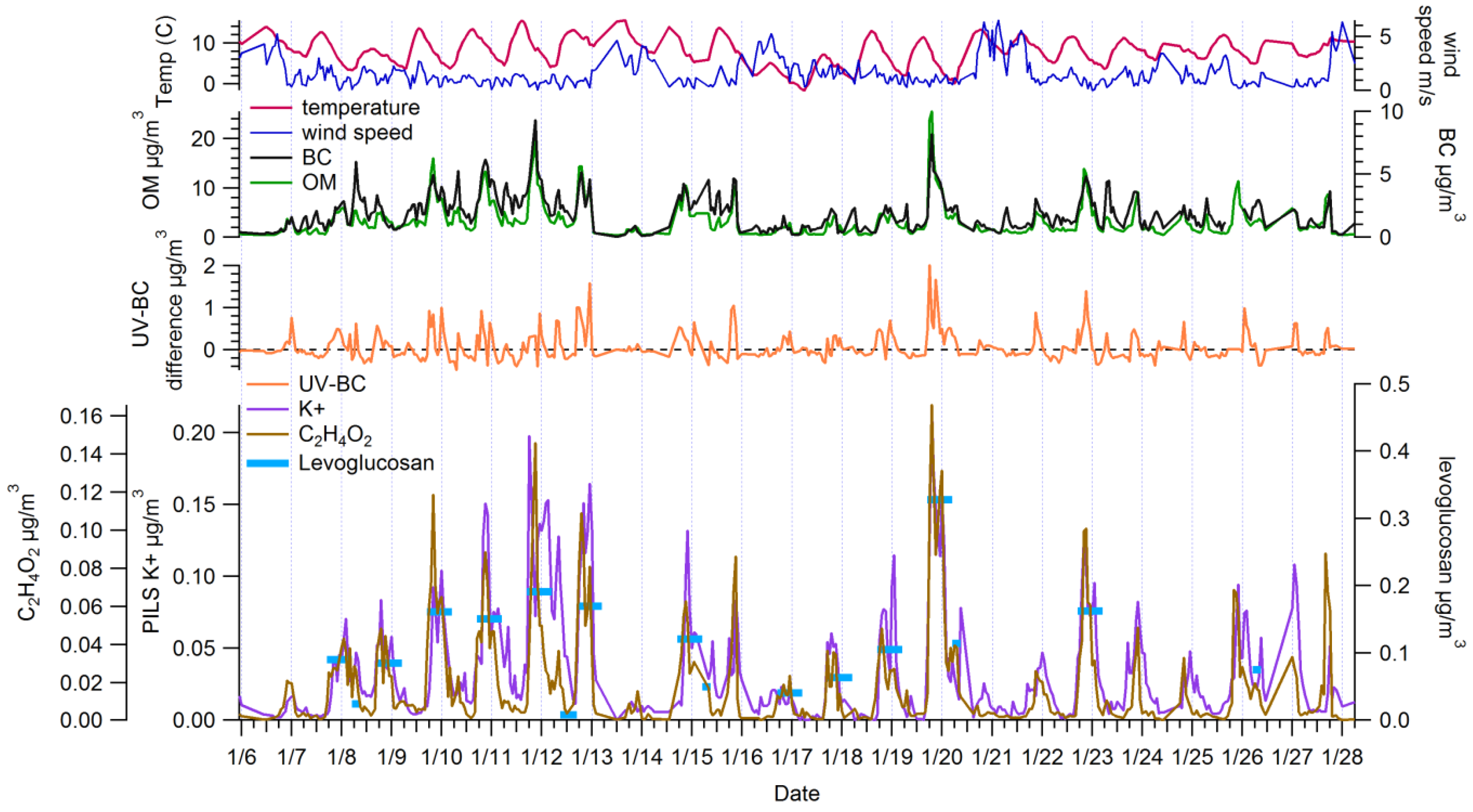
3.1. Ambient Concentrations and Temporal Variability of Biomass Burning Markers

Concentrations of organic matter, black carbon, and biomass burning indicators (levoglucosan, C2H4O2+, K+, and UV-BC difference) varied widely during January 2008, typically reaching a peak in the early evening (i.e., 1900 through 2100 LST). Figure 1 shows a time series for these species. OM at our roadside site was 3.3 µg/m3 on average, while BC was 1.8 µg/m3. Other aerosol and gaseous species were also measured and are summarized elsewhere [47]; in January 2008, OM and BC comprised 74% of the PM1 mass measured via the AMS and Aethalometer (excluding metals and crustal material which were not measured). C2H4O2+ concentrations averaged 0.018 µg/m3, and between 1800 and 0000 LST were nearly three times higher at 0.040 µg/m3. PILS K+ concentrations averaged 0.033 µg/m3 across the month of measurements, while levoglucosan concentrations during the 12-h overnight samples averaged 0.14 µg/m3. For comparison, the concentrations of elemental potassium at the Chemical Speciation Network (CSN) site in Las Vegas were 0.03 µg/m3 across five measurement days that fell within our study period.
Figure 2 summarizes the typical diurnal pattern of the semi-continuous measurements. BC concentrations were similar in the morning and evening, during the rush hour commute times. OM showed a minor peak in the morning, and was on average three times higher in the evening than in the morning. See Supplementary Materials Figures S1 and S2 for diurnal box plots of OM and BC. C2H4O2+, K+, and UV-BC difference all show a similar average diurnal pattern with a concentration peak extending from early evening through late night. K+ concentrations decrease more slowly than C2H4O2+ after midnight, possibly suggesting that C2H4O2+ is being lost via other mechanisms (such as partitioning from particle to gas phase or atmospheric reactions) than those affecting the nonvolatile and non-reactive species K+. K+, C2H4O2+, and UV-BC difference are all lowest in the midday, when emissions of residential biomass burning are low, wind speeds and dispersion are higher, and OM is lower.
OM has a similar pattern as these BB indicators, while BC has a different pattern; concentrations of BC reach comparable average maxima in the morning and evening. The diurnal pattern of BC indicates that mobile source emissions related to rush hour traffic are likely the most important source of BC. The diurnal OM pattern—low concentrations in the midday and a steep rise in concentrations in the evening—is likely due to a mix of fresh emissions in the morning and evening with the rush hour and other activities, plus an additional evening source of biomass burning. This was further demonstrated with PMF analyses on the AMS data [47], which showed that fresh, hydrocarbon-like organic aerosol (HOA) was present in the morning and evening, and that additional semi-volatile oxidized organic aerosol (SV-OOA) and BBOA were evident during the evening peak.

3.2. Comparison among Biomass Burning Markers

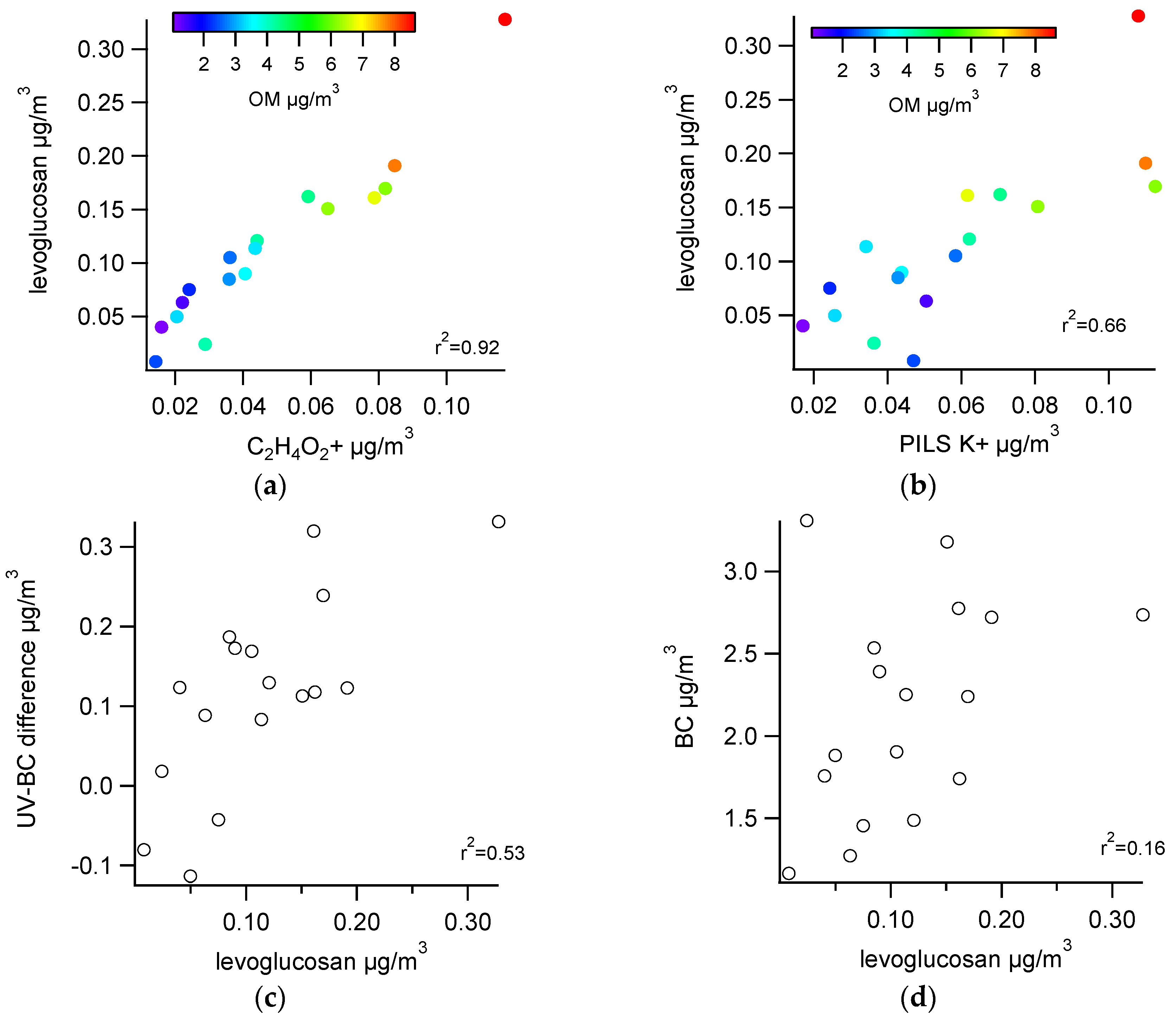
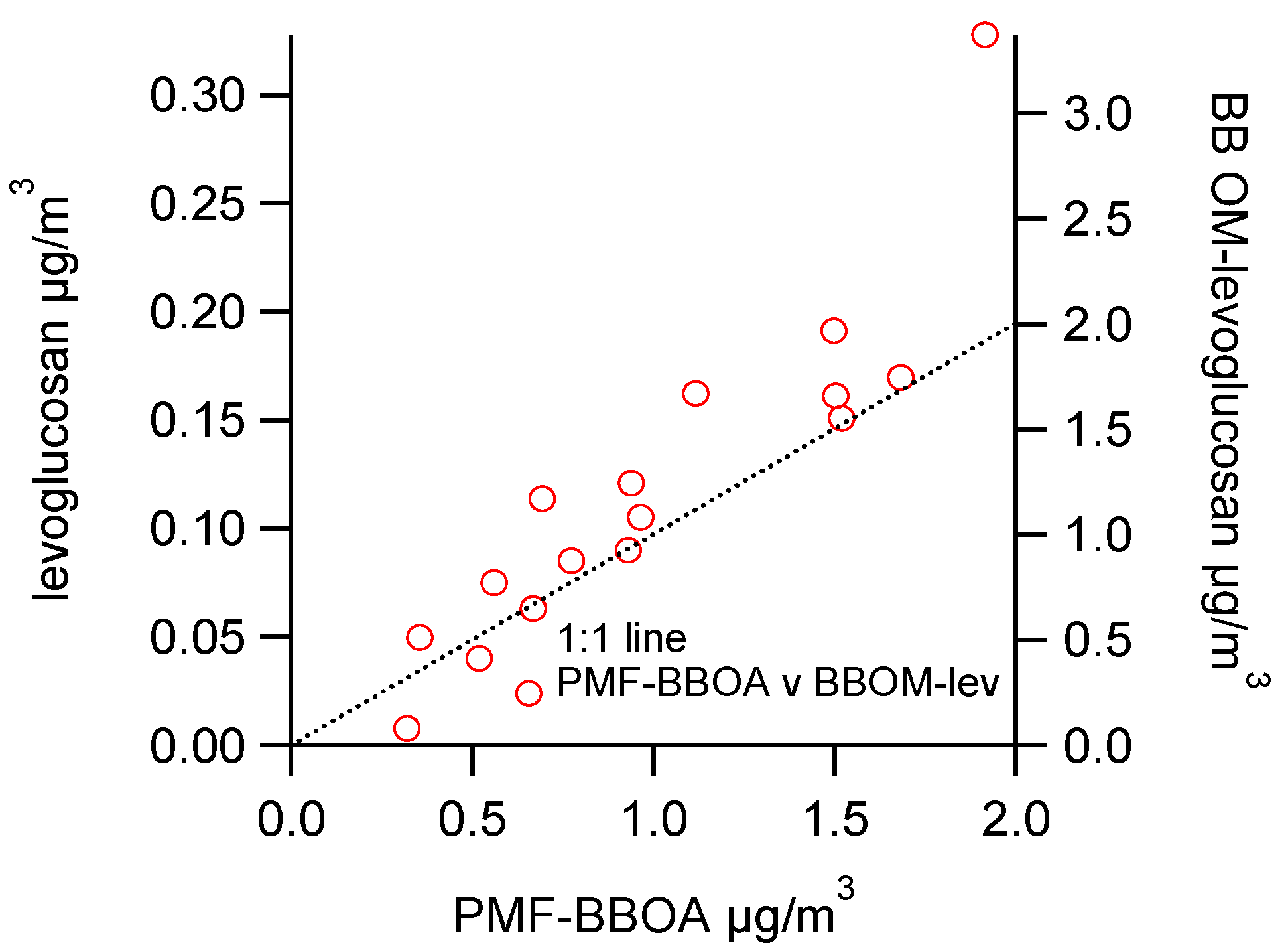
3.2.1. Comparisons with Levoglucosan

There was a range in how well the potential biomass burning indicators correlated with each other. Filter-based levoglucosan was available only for a subset of times during the study, at varying intervals. Correlations of filter-based levoglucosan with other measurements are summarized in Figure 3, while correlation among semi-continuous measurements from other instruments is discussed in the next section.
Levoglucosan concentrations measured from filters had high correlations with AMS C2H4O2+ (r2 = 0.92). This is expected, since C2H4O2+ is a fragment from levoglucosan and other co-emitted anhydrous sugars; pure levoglucosan introduced into an AMS yields a suite of ions that has C2H4O2+ as 13%–14% of the total ion fragment pattern [25]. In contrast, there was only a moderate correlation of PILS K+ (r2 = 0.66) or UV-BC difference (r2 = 0.53) with levoglucosan; no correlation was seen between levoglucosan and BC (r2 = 0.16). The lower correlations are perhaps not surprising, as both BC and K+ have other non-biomass burning sources; further, levoglucosan may be depleted during the 12-h sampling period via atmospheric reactions or phase partitioning to the gas phase, while BC and K+ would not undergo similar processes. BC and K+ are emitted primarily during flaming combustion, while levoglucosan is emitted more during smoldering combustion [25], which may also cause the lower correlation. The very low correlation with BC is likely because BC next to a roadway is predominantly from mobile sources, rather than from biomass burning. The modest correlation of levoglucosan with UV-BC difference, in the context of no correlation with BC, indicates that the UV-BC difference can be indicative of biomass burning aerosol, even when total BC is overwhelmingly from traffic-related sources.

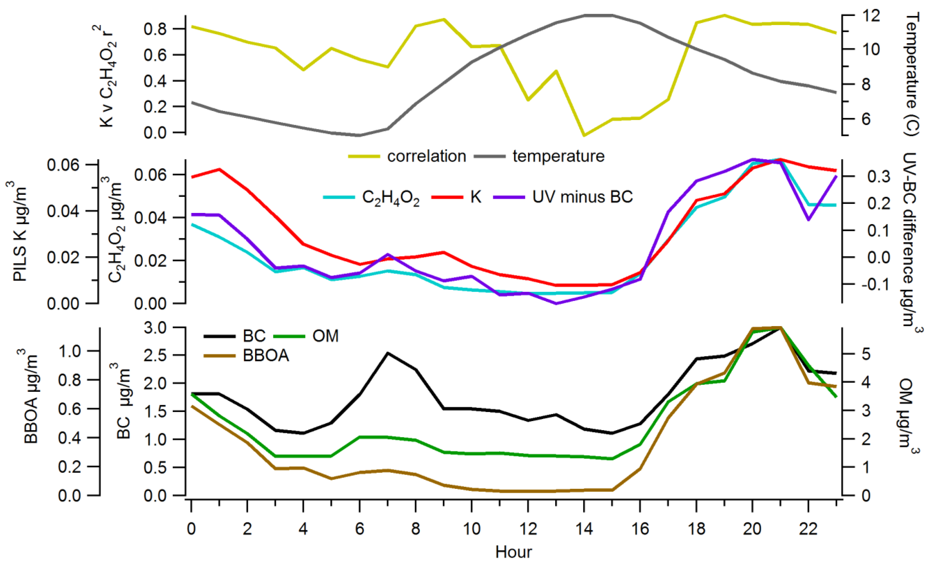
3.2.2. Comparisons among Semi-Continuous Biomass Burning Markers

While there are a limited number of multi-hour samples of levoglucosan, the high correlation between levoglucosan and C2H4O2+ confirms that C2H4O2+ is an excellent tracer for levoglucosan and biomass burning emissions. We next examined correlations of hourly averaged C2H4O2+ concentrations with K+, UV-BC difference values, and BC. Scatter plots of semi-continuous measurements are provided in Supplementary Materials Figure S2. As indicated by similar diurnal patterns, the measurements of biomass burning indicators were somewhat correlated, with some differences between species and time of day. The overall correlation coefficient (r2) between K+ and C2H4O2+ was 0.56, but if the correlations are examined by time of day, there is a large range in this correlation coefficient (Figure 2). Between 1800 and 0000 LST, when fresh biomass burning emissions are most likely, the correlation coefficient between K+ and C2H4O2+ was 0.84; it slowly decreased through the morning until 1200 through 1600 LST, when the correlation coefficient was 0.19. Midday, when the correlation is lowest, is also when concentrations are lowest and approaching the detection limit; the lower correlations may simply be due to increased measurement noise closer to the detection limits.
UV-BC difference had only a modest correlation with C2H4O2+ (r2 = 0.43), similar to the correlation between UV-BC difference and levoglucosan (r2 = 0.53). BC and C2H4O2+ have a good correlation during the evening (r2 = 0.80) during the period of strong residential wood combustion, but only a modest correlation in the morning (r2 = 0.35). K+ correlated poorly with both BC and UV-BC difference.
Overall, these results suggest that K+ and UV-BC difference are only modestly good indicators of biomass burning in Las Vegas next to a roadway, probably at least in part because there are other sources of K+ and BC at the monitoring site. It is clearly plausible that the majority of BC is from traffic-related emissions, which may complicate the relationship between UV-BC difference and levoglucosan or C2H4O2+. For K+, the modest correlation with levoglucosan or C2H4O2+ may be due to differences in emissions of these species during flaming and smoldering processes, or to minor sources of K+ confounding the relationship.

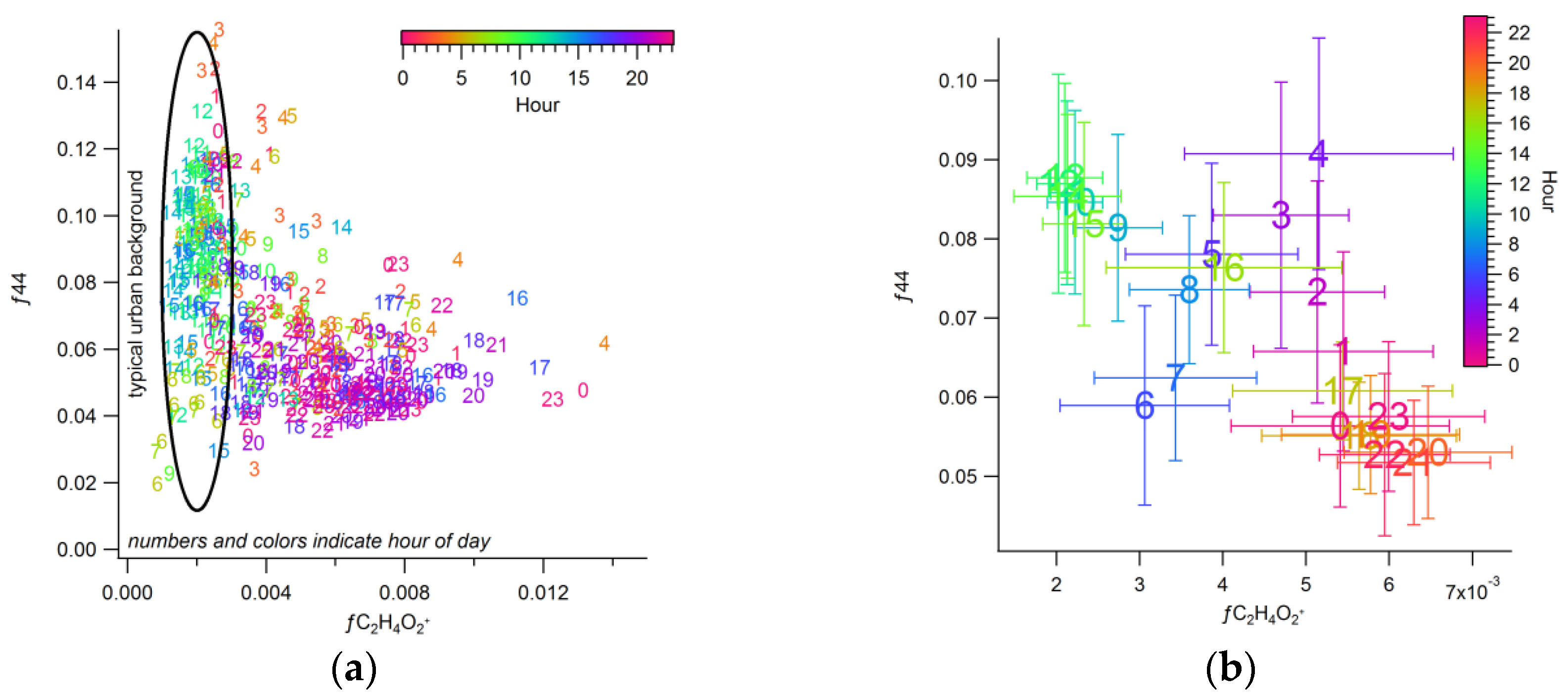
3.2.3. Urban Background Levels of C2H4O2+

There is a clear, strong relationship of levoglucosan with C2H4O2+ in the data here and in prior studies [25]. However, non-biomass burning sources, including organic acids, also can contribute to C2H4O2+ [28]. Lee et al. suggested that there is a background level of C2H4O2+, so that even when biomass burning is null, there is still some small concentration of C2H4O2+, approximately 0.3% of OA. This background C2H4O2+ can be seen in Figure 4, which shows the fraction of OM from C2H4O2+ (fC2H4O2+) vs. the fraction from m/z 44 (f44). During the morning and midday hours, a background of C2H4O2+ is evident of approximately 0.25% of the OM; during the evening, the fraction of mass from m/z 44 is much lower and the fraction from C2H4O2+ is much higher. Figure 4b shows how the relationship between m/z 44 and C2H4O2+ progresses, with a low m/z 44 fraction and C2H4O2+ fraction in the morning, followed by a midday increase in m/z 44 fraction, and an evening increase in C2H4O2+ fraction and decrease of m/z 44 fraction. This further shows the important contribution of biomass burning during the evening only, while other primary and secondary sources contribute to OM throughout the day.

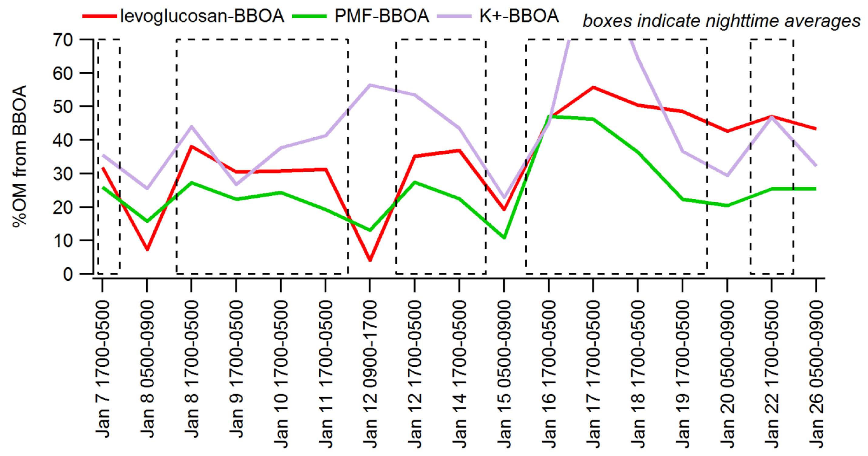
3.3. Apportioning Biomass Burning via Multiple Methods

With the suite of biomass burning tracers observed here, multiple methods are available to apportion the contribution of biomass burning to OM: (1) use PMF-AMS, applying PMF to the AMS data to determine contributing factors, including BBOA [63,64], and comparing to the (C2H4O2+ × OM)−1 ratio reported in laboratory source experiments for biomass burning fuels [25]; (2) use a (levoglucosan/OC)−1 ratio as reported in filter-based source profiles, estimating the amount of OC from the levoglucosan concentrations and using an assumed OM/OC ratio to estimate BBOA contributions to OM; and (3) use the same process as for Method 2, but using potassium from PILS and source profiles. Since Methods 2 and 3 rely on source profiles, these methods should estimate primary emissions, if the source profiles represent only primary emissions. The PMF factor approach in Method 1 may include primary and some secondary aerosol formation associated with BBOA. However, the PMF method could underestimate secondary OA from biomass burning in the obtained BBOA factor if the secondary OA is chemically more similar to SV-OOA than to primary BBOA. Since SV-OOA concentrations observed here are typically concurrent with and higher than BBOA, secondary OA associated with biomass burning emissions may not be fully captured in the BBOA factor. With only three PMF factors, i.e., with no SV-OOA factor, BBOA is higher than when four factors are used; it may be that with three factors, more of the secondary OA associated with biomass burning is contained in the BBOA factor. Table 1 summarizes the fraction of OM apportioned via each method. Brown et al. report the results from the PMF-AMS method where, using unit mass resolution AMS data and the EPA PMF program, on average 12% of the OM was attributable to biomass burning organic aerosol (BBOA) [47]. During overnight periods, BBOA was on average 26% of the OM.
A number of studies have reported a range of OM/C2H4O2+ ratios from source experiments. Lee et al. report a value of 34.5 for the OM/C2H4O2+ ratio generated in biomass burning experiments [25]. Alfarra et al. used a combination of PMF and 14C analyses to determine a similar ratio for OM to m/z 60, equal to 36, for wintertime wood combustion in Zurich, and suggested this ratio as a conservative estimate for apportioning BBOA [22]. The ratio of 34.5 is very close to the OM/C2H4O2+ ratio in the BBOA factor found here, which is 34.1, indicating that the BBOA factor is consistent with BBOA found in specific experiments where biomass burning is the main source of OA. In our PMF-AMS results, when using just three PMF factors, BBOA also comprises an average of 15% of the OM.
Fine et al. report an OC/levoglucosan ratio of 7.35 and an OC/K ratio of 20.83 for residential biomass burning emissions, used here to apportion BB OC based on our filter levoglucosan and PILS potassium measurements [38]. Recent studies have reported a wider range of levoglucosan/OC and K/OC emission ratios depending on biomass fuel type and burn conditions [16,29,65]. The 7.35 value for OC/levoglucosan is representative of fireplace combustion of hardwoods, which is likely appropriate for the Las Vegas area. Schmidl et al. developed a similar factor for Austrian fuels of 7.1 based on test burns in a tiled stove [66]. Puxbaum et al. [65] suggest an OM/OC conversion factor of 1.4 based on their calculations from the data reported in Fine et al. [11]. During the wintertime evening in Las Vegas, when biomass burning is most prevalent, the average OM/OC ratio is 1.46 [67], so a value of 1.4 for biomass burning appears reasonable. This yields a conversion of biomass burning OM equal to levoglucosan × 7.35 × 1.4. For potassium, biomass burning OM is calculated as K+ × 20.83 × 1.4.
Figure 5 shows the fraction of OM by each method for periods when levoglucosan data are available. Figure 6 compares PMF-BBOA with levoglucosan measurements and levoglucosan-BBOA apportionment. Using conversions from levoglucosan, 33% of the OM is from biomass burning during the overnight periods. This range is slightly higher than the 26% apportioned via 4-factor PMF-AMS. Estimates of K-based BBOA are higher, with 44% of the OM apportioned to BBOA during the 12-h overnight periods with levoglucosan data, and 26% on all evenings. All but the highest levoglucosan concentration data points fall about the 1:1 line between PMF-BBOA and levoglucosan-BBOA in Figure 6, and on most evenings the PMF and levoglucosan apportionment methods yield a similar result. Apportionment via K+ is consistently higher than all other methods. Each of the methods used has underlying uncertainties, in particular the selection of source profiles, since emissions of levoglucosan, K+, and OM vary by wood type, flaming vs. smoldering etc. Results in Table 1 capture some of this uncertainty, showing that the K+ method is the most uncertain compared to levoglucosan and AMS PMF.
One difficulty with comparing 12-h average apportionments via levoglucosan and K+ is that they may be lost at different rates by atmospheric processes [28], or emitted at varying rates as burning goes from flaming to smoldering [25]. In addition, as emissions age, gas/particle partitioning of semivolatile material may mean that the relationship of levoglucosan to OM emitted changes over time, as organic material is either condensed into the particle phase or partitioned in the vapor phase [17,28,68]. We examined the hourly average ratio and correlation between K+ and C2H4O2+ to understand how the relationship varies during the night (Figure 2). Between 1900 and 2300 LST, the ratio (0.625) and correlation (r2 = 0.80) between K+ and C2H4O2+ is consistent, but it degrades after 0000 LST, which is likely around the time that emissions have nearly stopped and levoglucosan may be lost via atmospheric reactions.
The sample with the highest disagreement between methods was the night of 19 January, when levoglucosan-BBOA and K-BBOA are similar (37%–39% of the OM) but are 1.6 times higher than PMF-BBOA. As seen in Figure 1, this was not only the evening of the highest levoglucosan and C2H4O2+ concentrations but also highest OM. It may be that PMF is under-predicting the amount of BBOA, since the OM concentration and possibly composition is quickly changing. The Q/Qexpected ratio and scaled residuals from PMF during this evening are low, indicating a good fit, but SV-OOA is also very high during this evening, so it is likely that some mass assigned by PMF as SV-OOA is actually BBOA. Since a constant profile is needed in PMF, differences in the BBOA composition between evenings mean that a “typical” or average profile is found; deviations from this profile suggest that mass appears to be apportioned to SV-OOA. However, as the results are consistent for all the other data points, our conclusion is that the three BBOA methods using levoglucosan and AMS data compare rather well most of the time. As there are other non-biomass burning sources of K+ in the area, and the amount of K+ emitted depends on the amount of flaming vs. smoldering emissions, assuming all the K+ is from biomass burning yields an upper limit of BBOA that is likely less accurate than the other methods used here.

4. Conclusions

Urban-scale biomass burning was found to be a surprising source of aerosol at Fyfe Elementary School in Las Vegas, even though the monitoring site was located next to a major freeway in a city with no tradition of home heating from wood stoves or fireplaces. Multiple methods of estimating the contribution of this source to fine PM were compared; HR-AMS measurements correlated with levoglucosan measurements, and both yielded similar estimates of total biomass burning organic aerosol (BBOA). Water-soluble potassium correlated with AMS C2H4O2+ only during evening hours, when biomass burning was relatively high; during other hours, there was little correlation, indicating that although K+ can be a useful biomass burning indicator when biomass burning is high, other sources tend to overwhelm the K+ concentrations during other hours. On average, BBOA comprised 9%–14% of the organic matter (OM), but was only significant during the evening hours, when OM was highest. During the overnight period between 1700 and 0500 LST, BBOA contributed between 26% and 33% of the OM (range derived from different analysis/measurement techniques). Thus, residential biomass burning is an unexpected, but relatively important, source of PM2.5 in Las Vegas.

Supplementary Materials

The following are available online at www.mdpi.com/2073-4433/7/4/58/s1, Figure S1: Diurnal box plot of HR-AMS OM (µg/m3); Figure S2: Diurnal box plot of Aethalometer BC (µg/m3).

Acknowledgments

Gary Norris and David Olson at EPA’s Office of Research and Development provided the chemical analysis of levoglucosan. Funding for the core measurements, including BC and meteorology, as well as for site operations, was provided by Nevada Department of Transportation. Sonoma Technology, Inc. (Petaluma, CA, USA), provided supplemental internal funding for the HR-AMS measurements. Lastly, we appreciate the review and comments from Steven G. Brown’s PhD committee on this work, including Sonia Kreidenweis, Colette Heald, and Anthony Marchese.

Author Contributions

Steven Brown, Paul Roberts, and Jeffrey Collett conceived and designed the experiments; Taehyoung Lee and Steven Brown performed the experiments; Steven Brown analyzed the data; Taehyoung Lee contributed analysis tools; Steven Brown wrote the paper.

Conflicts of Interest

The authors declare no conflict of interest. The funding sponsors had no role in the design of the study; in the collection, analyses, or interpretation of the data; in the writing of the manuscript; and in the decision to publish the results.

References

  1. Bergauff, M.A.; Ward, T.J.; Noonan, C.W.; Palmer, C.P. The effect of a woodstove changeout on ambient levels of PM2.5 and chemical tracers for woodsmoke in Libby, Montana. Atmos Environ. 2009, 43, 2938–2943. [Google Scholar] [CrossRef]
  2. Ward, T.; Noonan, C. Results of a residential indoor PM2.5 sampling program before and after a woodstove changeout. Indoor Air 2008, 18, 408–415. [Google Scholar] [CrossRef] [PubMed]
  3. Allen, G.A.; Miller, P.J.; Rector, L.J.; Brauer, M.; Su, J.G. Characterization of valley winter woodsmoke concentrations in Northern NY using highly time-resolved measurements. Aerosol Air Qual. Res. 2011, 11, 519–530. [Google Scholar] [CrossRef]
  4. Wang, Y.; Hopke, P.K.; Utell, M.J. Urban-scale spatial-temporal variability of black carbon and winter residential wood combustion particles. Aerosol Air Qual. Res. 2011, 11, 473–481. [Google Scholar] [CrossRef]
  5. Lighty, J.S.; Veranth, J.M.; Sarofim, A.F. Combustion aerosols: Factors governing their size and composition and implications to human health. J. Air Waste Manag. Assoc. 2000, 50, 1565–1618. [Google Scholar] [CrossRef] [PubMed]
  6. Barregard, L.; Sallsten, G.; Andersson, L.; Almstrand, A.-C.; Gustafson, P.; Andersson, M.; Olin, A.-C. Experimental exposure to wood smoke: Effects on airway inflammation and oxidative stress. Occup. Environ. Med. 2007, 65, 319–324. [Google Scholar] [CrossRef] [PubMed]
  7. Freeman, L.; Stiefer, P.S.; Weir, B.R. Carcinogenic Risk and Residential Wood Smoke; Systems Applications International: San Rafael, CA, USA, 1992. [Google Scholar]
  8. Seagrave, J.; McDonald, J.D.; Bedrick, E.; Edgerton, E.S.; Gigliotti, A.P.; Jansen, J.J.; Ke, L.; Naeher, L.P.; Seilkop, S.K.; Zheng, M.; et al. Lung toxicity of ambient particulate matter from southeastern U.S. sites with different contributing sources: Relationships between composition and effects. Environ. Health Perspect. 2006, 114, 1387–1393. [Google Scholar] [CrossRef] [PubMed]
  9. Travis, C.C.; Etnier, E.L.; Meyer, H.R. Health risks of residential wood heat. Environ. Manag. 1985, 9, 209–215. [Google Scholar] [CrossRef]
  10. Naeher, L.P.; Brauer, M.; Lipsett, M.; Zelikoff, J.T.; Simpson, C.D.; Koenig, J.Q.; Smith, K.R. Woodsmoke health effects: A review. Inhal. Toxicol. 2007, 19, 67–106. [Google Scholar] [CrossRef] [PubMed]
  11. Fine, P.M.; Cass, G.R.; Simoneit, B.R.T. Chemical characterization of fine particle emissions from the fireplace combustion of wood types grown in the Midwestern and Western United States. Environ. Eng. Sci. 2004, 21, 387–409. [Google Scholar] [CrossRef]
  12. Simoneit, B.R.T.; Schauer, J.J.; Nolte, C.G.; Oros, D.R.; Elias, V.O.; Fraser, M.P.; Rogge, W.F.; Cass, G.R. Levoglucosan, a tracer for cellulose in biomass burning and atmospheric particles. Atmos. Environ. 1999, 33, 173–182. [Google Scholar] [CrossRef]
  13. Simoneit, B.R.T. Biomass burning—A review of organic tracers for smoke from incomplete combustion. Appl. Geochem. 2002, 17, 129–162. [Google Scholar] [CrossRef]
  14. Engling, G.; Herckes, P.; Kreidenweis, S.M.; Malm, W.C.; Collett, J.L. Composition of the fine organic aerosol in Yosemite National Park during the 2002 Yosemite Aerosol Characterization Study. Atmos. Environ. 2006, 40, 2959–2972. [Google Scholar] [CrossRef]
  15. Schauer, J.J.; Kleeman, M.J.; Cass, G.R.; Simoneit, B.R.T. Measurement of emissions from air pollution sources. 3. C1 through C29 organic compounds from fireplace combustion of wood. Environ. Sci. Technol. 2001, 35, 1716–1728. [Google Scholar] [CrossRef] [PubMed]
  16. Sullivan, A.P.; Holden, A.S.; Patterson, L.A.; McMeeking, G.R.; Kreidenweis, S.M.; Malm, W.C.; Hao, W.M.; Wold, C.E.; Collett, J.L., Jr. A method for smoke marker measurements and its potential application for determining the contribution of biomass burning from wildfires and prescribed fires to ambient PM2.5 organic carbon. J. Geophys. Res. 2008. [Google Scholar] [CrossRef]
  17. Hennigan, C.J.; Miracolo, M.A.; Engelhart, G.J.; May, A.A.; Presto, A.A.; Lee, T.; Sullivan, A.P.; McMeeking, G.R.; Coe, H.; Wold, C.E.; et al. Chemical and physical transformations of organic aerosol from the photo-oxidation of open biomass burning emissions in an environmental chamber. Atmos. Chem. Phys. 2011, 11, 7669–7686. [Google Scholar] [CrossRef]
  18. Hoffmann, D.; Tilgner, A.; Iinuma, Y.; Herrmann, H. Atmospheric stability of levoglucosan: A detailed laboratory and modeling study. Environ. Sci. Technol. 2010, 44, 694–699. [Google Scholar] [CrossRef] [PubMed]
  19. Slade, J.H.; Knopf, D.A. Multiphase OH oxidation kinetics of organic aerosol: The role of particle phase state and relative humidity. Geophys. Res. Lett. 2014, 41, 5297–5306. [Google Scholar] [CrossRef]
  20. Kessler, S.H.; Smith, J.D.; Che, D.L.; Worsnop, D.R.; Wilson, K.R.; Kroll, J.H. Chemical sinks of organic aerosol: Kinetics and products of the heterogeneous oxidation of erythritol and levoglucosan. Environ. Sci. Technol. 2010, 44, 7005–7010. [Google Scholar] [CrossRef] [PubMed]
  21. Slade, J.H.; Knopf, D.A. Heterogeneous OH oxidation of biomass burning organic aerosol surrogate compounds: Assessment of volatilisation products and the role of OH concentration on the reactive uptake kinetics. Phys. Chem. Chem. Phys. 2013, 15, 5898–5915. [Google Scholar] [CrossRef] [PubMed]
  22. Alfarra, M.R.; Prévôt, A.S.H.; Szidat, S.; Sandradewi, J.; Weimer, S.; Lanz, V.A.; Schreiber, D.; Mohr, M.; Baltensperger, U. Identification of the mass spectral signature of organic aerosols from wood burning emissions. Environ. Sci. Technol. 2007, 41, 5770–5777. [Google Scholar] [CrossRef] [PubMed]
  23. Weimer, S.; Alfarra, M.R.; Schreiber, D.; Mohr, M.; Prévôt, A.S.H.; Baltensperger, U. Organic aerosol mass spectral signatures from wood-burning emissions: Influence of burning conditions and wood type. J. Geophys. Res. Atmos. 2008. [Google Scholar] [CrossRef]
  24. Schneider, J.; Weimer, S.; Drewnick, F.; Borrmann, S.; Helas, G.; Gwaze, P.; Schmid, O.; Andreae, M.O.; Kirchner, U. Mass spectrometric analysis and aerodynamic properties of various types of combustion-related aerosol particles. Int. J. Mass Spec. 2006, 258, 37–49. [Google Scholar] [CrossRef]
  25. Lee, T.; Sullivan, A.P.; Mack, L.; Jimenez, J.L.; Kreidenweis, S.M.; Onasch, T.B.; Worsnop, D.R.; Malm, W.; Wold, C.E.; Hao, W.M.; et al. Chemical smoke marker emissions during flaming and smoldering phases of laboratory open burning of wildland fuels. Aerosol Sci. Technol. 2010. [Google Scholar] [CrossRef]
  26. Mohr, C.; Huffman, J.A.; Cubison, M.; Aiken, A.C.; Docherty, K.S.; Kimmel, J.R.; Ulbrich, I.M.; Hannigan, M.; Jimenez, J.L. Characterization of primary organic aerosol emissions from meat cooking, trash burning, and motor vehicles with high-resolution aerosol mass spectrometry and comparison with ambient and chamber observations. Environ. Sci. Technol. 2009, 43, 2443–2449. [Google Scholar] [CrossRef] [PubMed]
  27. Takegawa, N.; Miyakawa, T.; Kawamura, K.; Kondo, Y. Contribution of selected dicarboxylic and omega-oxocarboxylic acids in ambient aerosol to the m/z 44 signal of an aerodyne aerosol mass spectrometer. Aerosol Sci. Technol. 2007, 41, 418–437. [Google Scholar] [CrossRef]
  28. Cubison, M.J.; Ortega, A.M.; Hayes, P.L.; Farmer, D.K.; Day, D.; Lechner, M.J.; Brune, W.H.; Apel, E.; Diskin, G.S.; Fisher, J.A.; et al. Effects of aging on organic aerosol from open biomass burning smoke in aircraft and laboratory studies. Atmos. Chem. Phys. 2011, 11, 12049–12064. [Google Scholar] [CrossRef]
  29. Minguillon, M.C.; Perron, N.; Querol, X.; Szidat, S.; Fahrni, S.M.; Alastuey, A.; Jimenez, J.L.; Mohr, C.; Ortega, A.M.; Day, D.A.; et al. Fossil versus contemporary sources of fine elemental and organic carbonaceous particulate matter during the DAURE campaign in Northeast Spain. Atmos. Chem. Phys. 2011, 11, 12067–12084. [Google Scholar] [CrossRef] [Green Version]
  30. Kim, E.; Larson, T.V.; Hopke, P.K.; Slaughter, C.; Sheppard, L.E.; Claiborn, C. Source identification of PM2.5 in an arid northwest U.S. city by positive matrix factorization. Atmos. Res. 2003, 66, 291–305. [Google Scholar] [CrossRef]
  31. Poirot, R. Tracers of Opportunity: Potassium. Available online: http://capita.wustl.edu/PMFine/Workgroup/SourceAttribution/Reports/In-progress/potass/Kcover.htm (accessed on 12 April 2016).
  32. Liu, W.; Wang, Y.; Russell, A.; Edgerton, E.S. Atmospheric aerosol over two urban-rural pairs in the southeastern United States: Chemical composition and possible sources. Atmos. Environ. 2005, 39, 4453–4470. [Google Scholar] [CrossRef]
  33. Brown, S.G.; Frankel, A.; Raffuse, S.M.; Roberts, P.T.; Hafner, H.R.; Anderson, D.J. Source apportionment of fine particulate matter in Phoenix, Arizona, using positive matrix factorization. J. Air Waste Manag. Assoc. 2007, 57, 741–752. [Google Scholar] [PubMed]
  34. Aiken, A.C.; de Foy, B.; Wiedinmyer, C.; DeCarlo, P.F.; Ulbrich, I.M.; Wehrli, M.N.; Szidat, S.; Prévôt, A.S.H.; Noda, J.; Wacker, L.; et al. Mexico City aerosol analysis during MILAGRO using high resolution aerosol mass spectrometry at the urban supersite (T0). Part 2: Analysis of the biomass burning contribution and the non-fossil carbon fraction. Atmos. Chem. Phys. 2010, 10, 5315–5341. [Google Scholar] [CrossRef] [Green Version]
  35. Zhang, X.; Hecobian, A.; Zheng, M.; Frank, N.H.; Weber, R.J. Biomass burning impact on PM2.5 over the southeastern US during 2007: Integrating chemically speciated FRM filter measurements, MODIS fire counts and PMF analysis. Atmos. Chem. Phys. 2010, 10, 6839–6853. [Google Scholar] [CrossRef]
  36. Schauer, J.J.; Kleeman, M.J.; Cass, G.R.; Simoneit, B.R.T. Measurement of emissions from air pollution sources. 1. C1 through C29 organic compounds from meat charbroiling. Environ. Sci. Technol. 1999, 33, 1566–1577. [Google Scholar] [CrossRef]
  37. Fine, P.M.; Cass, G.R.; Simoneit, B.R.T. Chemical characterization of fine particle emissions from the fireplace combustion of woods grown in the southern United States. Environ. Sci. Technol. 2002, 36, 1442–1451. [Google Scholar] [CrossRef] [PubMed]
  38. Fine, P.M.; Cass, G.R.; Simoneit, B.R.T. Organic compounds in biomass smoke from residential wood combustion: Emissions characterization at a continental scale. J. Geophys. Res. Atmos. 2002. [Google Scholar] [CrossRef]
  39. Fine, P.M.; Cass, G.R.; Simoneit, B.R.T. Chemical characterization of fine particle emissions from fireplace combustion of woods grown in the northeastern United States. Environ. Sci. Technol. 2001, 35, 2665–2675. [Google Scholar] [CrossRef] [PubMed]
  40. Allen, G.A.; Lawrence, J.; Koutrakis, P. Field validation of a semi-continuous method for aerosol black carbon (Aethalometer) and termporal patterns of summertime hourly black carbon measurements in Southwestern Pennsylvania. Atmos. Environ. 1999, 33, 817–823. [Google Scholar] [CrossRef]
  41. Sandradewi, J.; Prévôt, A.S.H.; Weingartner, E.; Schmidhauser, R.; Gysel, M.; Baltensperger, U. A study of wood burning and traffic aerosols in an Alpine valley using a multi-wavelength Aethalometer. Atmos. Environ. 2008, 42, 101–112. [Google Scholar] [CrossRef]
  42. Harrison, R.M.; Beddowsa, D.C.S.; Jones, A.M.; Calvo, A.; Alves, C.; Pio, C. An evaluation of some issues regarding the use of aethalometers to measure woodsmoke concentrations. Atmos. Environ. 2013, 80, 540–548. [Google Scholar] [CrossRef]
  43. Sandradewi, J.; Prévôt, A.S.H.; Alfarra, M.R.; Szidat, S.; Wehrli, M.N.; Ruff, M.; Weimer, S.; Lanz, V.A.; Weingartner, E.; Perron, N.; et al. Comparison of several wood smoke markers and source apportionment methods for wood burning particulate mass. Atmos. Chem. Phys. Discuss. 2008, 8, 8091–8118. [Google Scholar] [CrossRef]
  44. Favez, O.; El Haddad, I.; Piot, C.; Boréave, A.; Abidi, E.; Marchand, N.; Jaffrezo, J.-L.; Besombes, J.-L.; Personnaz, M.-B.; Sciare, J.; et al. Inter-comparison of source apportionment models for the estimation of wood burning aerosols during wintertime in an Alpine city (Grenoble, France). Atmos. Chem. Phys. 2010, 10, 5295–5314. [Google Scholar] [CrossRef] [Green Version]
  45. Green, M.C.; Chow, J.C.; Hecobian, A.; Etyemezian, V.; Kuhns, H.; Watson, J.G. Las Vegas Valley Visibility and PM2.5 Study; Final Report Prepared for the Clark County Department of Air Quality Management, Las Vegas, NV; Desert Research Institute: Las Vegas, NV, USA, 2002. [Google Scholar]
  46. Watson, J.G.; Barber, P.W.; Chang, M.C.O.; Chow, J.C.; Etyemezian, V.R.; Green, M.C.; Keislar, R.E.; Kuhns, H.D.; Mazzoleni, C.; Moosmüller, H.; et al. Southern Nevada Air Quality Study; Final Report Prepared for the U.S. Department of Transportation, Washington, DC; Desert Research Institute: Reno, NV, USA, 2007. [Google Scholar]
  47. Brown, S.G.; Lee, T.; Norris, G.A.; Roberts, P.T.; Collett, J.L., Jr.; Paatero, P.; Worsnop, D.R. Receptor modeling of near-roadway aerosol mass spectrometer data in Las Vegas, Nevada, with EPA PMF. Atmos. Chem. Phys. 2012, 12, 309–325. [Google Scholar] [CrossRef] [Green Version]
  48. Brown, S.G.; McCarthy, M.C.; DeWinter, J.L.; Vaughn, D.L.; Roberts, P.T. Changes in air quality at near-roadway schools after a major freeway expansion in Las Vegas, Nevada. J. Air Waste Manag. Assoc. 2014, 64, 1002–1012. [Google Scholar] [CrossRef]
  49. DeCarlo, P.; Kimmel, J.R.; Trimborn, A.; Northway, M.; Jayne, J.T.; Aiken, A.C.; Gonin, M.; Fuhrer, K.; Horvath, T.; Docherty, K.S.; et al. Field-deployable, high-resolution, time-of-flight aerosol mass spectrometer. Anal. Chem. 2006, 78, 8281–8289. [Google Scholar] [CrossRef] [PubMed]
  50. Jimenez, J.L.; Jayne, J.T.; Shi, Q.; Kolb, C.E.; Worsnop, D.R.; Yourshaw, I.; Seinfeld, J.H.; Flagan, R.C.; Zhang, X.F.; Smith, K.A.; et al. Ambient aerosol sampling using the Aerodyne Aerosol Mass Spectrometer. J. Geophys. Res. Atmos. 2003. [Google Scholar] [CrossRef]
  51. Zhang, Q.; Jimenez, J.L.; Canagaratna, M.R.; Ulbrich, I.M.; Ng, N.L.; Worsnop, D.R.; Sun, Y. Understanding atmospheric organic aerosols via factor analysis of aerosol mass spectrometry: A review. Anal. Bioanal. Chem. 2011, 401, 3045–3067. [Google Scholar] [CrossRef] [PubMed]
  52. Sun, Y.; Zhang, Q.; MacDonald, A.M.; Hayden, K.; Li, S.M.; Liggio, J.; Liu, P.S.K.; Anlauf, K.G.; Leaitch, W.R.; Steffen, A.; et al. Size-resolved aerosol chemistry on Whistler Mountain, Canada with a high-resolution aerosol mass spectrometer during INTEX-B. Atmos. Chem. Phys. 2009, 9, 3095–3111. [Google Scholar] [CrossRef]
  53. Canagaratna, M.R.; Jayne, J.T.; Jimenez, J.L.; Allan, J.D.; Alfarra, M.R.; Zhang, Q.; Onasch, T.B.; Drewnick, F.; Coe, H.; Middlebrook, A.; et al. Chemical and microphysical characterization of ambient aerosols with the aerodyne aerosol mass spectrometer. Mass Spectrom. Rev. 2007, 26, 185–222. [Google Scholar] [CrossRef] [PubMed]
  54. Drewnick, F.; Hings, S.S.; Alfarra, M.R.; Prevot, A.S.H.; Borrmann, S. Aerosol quantification with the Aerodyne Aerosol Mass Spectrometer: Detection limits and ionizer background effects. Atmos. Measure. Tech. 2009, 2, 33–46. [Google Scholar] [CrossRef]
  55. Olson, D.A.; Vedantham, R.; Norris, G.A.; Brown, S.G.; Roberts, P. Determining source impacts near roadways using wind regression and organic source markers. Atmos. Environ. 2012, 47, 261–268. [Google Scholar] [CrossRef]
  56. Orsini, D.A.; Ma, Y.L.; Sullivan, A.; Sierau, B.; Baumann, K.; Weber, R.J. Refinements to the particle-into-liquid sampler (PILS) for ground and airborne measurements of water soluble aerosol composition. Atmos. Environ. 2003, 37, 1243–1259. [Google Scholar] [CrossRef]
  57. Weber, R.J.; Orsini, D.; Daun, Y.; Lee, Y.N.; Klotz, P.J.; Brechtel, F. A particle-into-liquid collector for rapid measurement of aerosol bulk chemical composition. Aerosol Sci. Technol. 2001, 35, 718–727. [Google Scholar] [CrossRef]
  58. Weber, R.; Orsini, D.; Duan, Y.; Baumann, K.; Kiang, C.S.; Chameides, W.; Lee, Y.N.; Brechtel, F.; Klotz, P.; Jongejan, P.; et al. Intercomparison of near real time monitors of PM2.5 nitrate and sulfate at the U.S. Environmental Protection Agency Atlanta Supersite. J. Geophys. Res. Atmos. 2003. [Google Scholar] [CrossRef]
  59. Sorooshian, A.; Brechtel, F.J.; Ma, Y.L.; Weber, R.J.; Corless, A.; Flagan, R.C.; Seinfeld, J.H. Modeling and characterization of a particle-into-liquid sampler (PILS). Aerosol Sci. Technol. 2006, 40, 396–409. [Google Scholar] [CrossRef]
  60. Lee, T.; Yu, X.-Y.; Kreidenweis, S.M.; Malm, W.C.; Collett, J.L. Semi-continuous measurement of PM2.5 ionic composition at several rural locations in the United States. Atmos. Environ. 2008, 42, 6655–6669. [Google Scholar] [CrossRef]
  61. Norris, G.; Duvall, R.; Brown, S.; Bai, S. EPA Positive Matrix Factorization (PMF) 5.0 Fundamentals and User Guide; Prepared for the U.S. Environmental Protection Agency Office of Research and Development: Washington, DC, USA, 2014. [Google Scholar]
  62. Brown, S.G.; Eberly, S.; Paatero, P.; Norris, G.A. Methods for estimating uncertainty in PMF solutions: Examples with ambient air and water quality data and guidance on reporting PMF results. Sci. Total Environ. 2015, 518, 626–635. [Google Scholar] [CrossRef] [PubMed]
  63. Ulbrich, I.M.; Canagaratna, M.R.; Zhang, Q.; Worsnop, D.R.; Jimenez, J.L. Interpretation of organic components from Positive Matrix Factorization of aerosol mass spectrometric data. Atmos. Chem. Phys. 2009, 9, 2891–2918. [Google Scholar] [CrossRef]
  64. Lanz, V.A.; Alfarra, M.R.; Baltensperger, U.; Buchmann, B.; Hueglin, C.; Prévôt, A.S.H. Source apportionment of submicron organic aerosols at an urban site by factor analytical modelling of aerosol mass spectra. Atmos. Chem. Phys. 2007, 7, 1503–1522. [Google Scholar] [CrossRef]
  65. Puxbaum, H.; Caseiro, A.; Sanchez-Ochoa, A.; Kasper-Giebl, A.; Claeys, M.; Gelencser, A.; Legrand, M.; Preunkert, S.; Pio, C. Levoglucosan levels at background sites in Europe for assessing the impact of biomass combustion on the European aerosol background. J. Geophys. Res. 2007. [Google Scholar] [CrossRef]
  66. Schmidl, C.; Marr, I.L.; Caseiro, A.; Kotianova, P.; Berner, A.; Bauer, H.; Kasper-Giebl, A.; Puxbaum, H. Chemical characterisation of fine particle emissions from wood stove combustion of common woods growing in mid-European Alpine regions. Atmos. Environ. 2008, 42, 126–141. [Google Scholar] [CrossRef]
  67. Brown, S.G.; Lee, T.; Roberts, P.T.; Collett, J.L., Jr. Variations in the OM/OC ratio of urban organic aerosol next to a major roadway. J. Air Waste Manag. Assoc. 2013, 63, 1422–1433. [Google Scholar] [CrossRef] [PubMed]
  68. Oja, V.; Suuberg, E.M. Vapor pressures and enthalpies of sublimation of d-glucose, d-xylose, cellobiose, and levoglucosan. J. Chem. Eng. Data 1999, 44, 26–29. [Google Scholar] [CrossRef]
Figure 1. Time series of temperature, wind speed, Aethalometer black carbon (BC), Aerosol Mass Spectrometer (AMS) organic matter (OM), Aethalometer UV-BC difference, PILS K+, AMS C2H4O2+, and levoglucosan from quartz fiber filters at Fyfe during January 2008 (all units in µg/m3 except temperature in degrees C and wind speed in m/s).
Atmosphere 07 00058 g001
Figure 2. Average concentration by hour (LST) for Aethalometer BC, AMS OM, PMF-BBOA, UV-BC difference, PILS K+, and AMS C2H4O2+ (all units µg/m3), plus correlation (r2) by hour of PILS K+ vs. AMS C2H4O2+ and temperature (degrees C).
Atmosphere 07 00058 g002
Figure 3. Scatter plots of levoglucosan concentrations (µg/m3) correlated with (a) AMS C2H4O2+ (µg/m3); (b) PILS K+ (µg/m3); (c) UV-BC difference (µg/m3); and (d) BC (µg/m3).
Atmosphere 07 00058 g003
Figure 4. Scatter plot of the fraction of OM from m/z 44 and C2H4O2+, with color and numbers indicating hour of the day, for: (a) all data (hourly averages); and (b) data averaged by hour during the study.
Atmosphere 07 00058 g004
Figure 5. Percentage of OM apportioned by four methods for each time period where levoglucosan was quantified; boxes indicate nighttime averages (1700–0500 LST). Not shown is K-BBOA value of 100% apportioned OM on 17 January 1700-0500.
Atmosphere 07 00058 g005
Figure 6. Comparison of PMF-BBOA concentrations vs. levoglucosan (primary y-axis) and BB OM by levoglucosan (secondary y-axis); all units are µg/m3.
Atmosphere 07 00058 g006
Table 1. Fraction and standard deviation of OM (fOM) apportioned during 12 overnight (1700–0500 LST) periods, January evenings, and over all hours, via PMF-AMS, levoglucosan, and K+. Apportionment by levoglucosan is available only for the 12 overnight filter sample periods.
Sample Range% OM from BB via Levoglucosan% OM from BB via PMF-AMS (BBOA)% OM via K+
12 12-h overnight periods33% +/− 7%26% +/− 9%44% +/− 18%
All evenings (1800–2300 LST)n/a15% +/− 9%26% +/− 24%
All hoursn/a9% +/− 8%25% +/− 25%

