Article

Long-Range Transport of SO2 from Continental Asia to Northeast Asia and the Northwest Pacific Ocean: Flow Rate Estimation Using OMI Data, Surface in Situ Data, and the HYSPLIT Model

1
Department of Spatial Information Engineering, Pukyong National University, Busan 608-737, Korea
2
Department of Urban Environmental Engineering, Kyungnam University, Changwon-si, Gyeongsangnam-do 631-701, Korea
*
Author to whom correspondence should be addressed.
Atmosphere 2016, 7(4), 53; https://doi.org/10.3390/atmos7040053
Submission received: 3 March 2016 / Revised: 31 March 2016 / Accepted: 1 April 2016 / Published: 8 April 2016

Abstract

:
This present study suggests a method to calculate the SO2 flow rate from a source area to receptor areas on a regional scale using Ozone Monitoring Instrument (OMI) SO2 products, surface in situ SO2 data, and the hybrid single particle Lagrangian integrated trajectory (HYSPLIT) model. The method was implemented to calculate the SO2 flow rate from continental Asia to northeast Asia and the Northwest Pacific Ocean. For the high SO2 events when SO2 was transported from continental Asia to Japan via the Korean Peninsula on 22–24 December 2006, the long-range transported SO2 flow rates were 14.0 (21.0) Mg·h−1 OMI·gird−1 at Gangneung (Seoul) in Korea and 4.2 (5.3) Mg·h−1 OMI·gird−1 at Hiroshima (Kumamoto) in Japan. For the long-range transport of SO2 from continental Asia to the Northwest Pacific Ocean on 6–7 October 2008 (9–11 October 2006), the flow rates were 16.1 (16.2) Mg·h−1 OMI·gird−1 at Hokkaido, Japan (Vladivostok, Russia) and 5.6 (16.7) Mg·h−1 OMI·gird−1 at the Aleutian Islands, Northwest Pacific Ocean (Bering Sea). The mean rates of decrease in the SO2 flow rate per 1000 km were also calculated between continental Asia and the receptor areas. Uncertainties in the flow rate estimates were also assessed and discussed.

1. Introduction

Sulfur dioxide (SO2) in the atmosphere is emitted from anthropogenic and natural sources [1,2,3,4,5]. More than 70% of the global total SO2 emission is from anthropogenic sources and half of this is from fossil-fuel combustion [6]. In last two decades, atmospheric SO2 has shown a decreasing trend in regions including North America and Europe [7]; however, the global total SO2 has increased due to increased fossil-fuel combustion in China [8,9]. Although China has started showing a decreasing trend in SO2 emission since 2008 [10], SO2 emission in China is still reported to account for more than 60% of the total Asian SO2 emission. Today, SO2 emission in China is reported to account for about 25% of the global total SO2 emission and more than 90% of the total East Asian SO2 emission [10,11].
Chemical reactions transform SO2 into sulfate and sulfuric acid [5]. These sulfuric species may directly degrade the local air quality in receptor areas while they also cause acid rain and poor visibility at the receptor areas via long-range transport (LRT) [12,13,14]. SO2 and various sulfuric aerosols are also known to affect radiative forcing [15]. Therefore, to establish effective air-quality control strategies at receptor areas, it is necessary to quantify the contribution of long-range transported air pollutants such as SO2 to the atmospheric environment of that area.
Recent studies have examined long-range transported SO2 (LRT-SO2) emitted from continental Asia and investigated its contribution to downwind regions. Some of these studies utilized SO2 data from satellite sensors that enable the investigation of SO2 LRT as they provide regional and global coverage over short time intervals from one to several days. Chemical transport models and the data obtained from aircraft and satellite (Moderate Resolution Imaging Spectroradiometer (MODIS), Multi-angle Imaging Spectroradiometer (MISR)) measurements have been utilized to estimate the contribution of LRT-SO2 from East Asia to North America [14]. The LRT of SO2 from continental Asia to the Korean Peninsula has been detected using data from the Scanning Imaging Absorption Spectrometer for Atmospheric Chartography (SCIAMACHY) and validated through comparison with Multi Axis Differential Optical Absorption Spectroscopy (MAX-DOAS) and in situ measurements [16]. The meteorological mechanisms of transport were reported based on aircraft observations over Northeast China [17]. Lu et al. [8] reported correlations between sulfur variations in East Asia and SO2 emissions in China using the Ozone Monitoring Instrument (OMI) and SCIAMACHY data. Jeong et al. [18] estimated the contribution of LRT-SO2 from China to increased SO2 concentration in Seoul using a Conditional Potential Source Contribution Function (CPSCF) with SO2 data obtained from OMI and in situ measurements. Hsu et al. [19] reported high SO2 events over the Pacific Ocean due to LRT from China, as inferred from OMI, Cloud-Aerosol Lidar and Infrared Pathfinder Satellite Observations (CALIPSO) data, and the hybrid single particle Lagrangian integrated trajectory (HYSPLIT) model. Mallik et al. [20] reported an episode of high SO2 concentration over Northern India as a result of LRT from Africa using OMI, CALIPSO, and backward trajectory analysis data. Li et al. [21] reported a case study of transport and evolution of a SO2 plume from Northern China using OMI, MODIS, and backward trajectory analysis data. The above studies revealed that LRT of SO2 and sulfuric species emitted in China and East Asia can affect not only neighboring areas but also remote regions such as the Pacific Ocean and North America. They either reported the detection of LRT-SO2 or estimated the contribution of LRT-SO2 to the surface SO2 concentration at receptor areas.
For better understanding of the LRT-SO2 contribution to changes in the SO2 amount at a receptor area, it is necessary to identify the total amount of LRT-SO2 at the receptor area, meaning, in turn, that we need to calculate LRT-SO2 flow rate. The flow rate information can be directly used to quantify the total LRT-SO2 amounts for a duration at a receptor area if it is obtained either hourly or daily by Low Earth Orbit (LEO) or geostationary orbit (GEO) satellite measurement, respectively. Here, SO2 flow rate denotes the mass of SO2 that passes per unit time. In the present study, we calculate the flow rate of LRT-SO2 from continental Asia to the Korean Peninsula, Japan, and the Northwest Pacific Ocean using OMI SO2 column data, in situ SO2 data, and HYSPLIT backward trajectory simulations. In addition, we investigate the changes in the LRT-SO2 flow rate as a function of distance from continental Asia. Uncertainties in the flow rate estimates are also discussed.

2. Method

2.1. Data

The SO2 column data used to calculate the flow rate of the LRT-SO2 were obtained from the OMI onboard NASA’s Earth Observing System (EOS)/Aura satellite [22] that was launched on 15 July 2004 in a sun-synchronous ascending polar orbit at 705 km altitude with 13:45 local equator crossing time. The details of the SO2 retrieval method have been described previously [23,24]. SO2 column data in the OMSO2e level-3 products (i.e., OMSO2e at a resolution of 0.25°) were acquired from NASA’s Goddard Earth Sciences Data and Information Services Center (GES-DISC) [25]. We used the SO2 data produced with the updated algorithm in 2015 [26]. We averaged six pixels of OMI PBL SO2 to enhance the accuracy (NASA’s Goddard Earth Sciences Data and Information Services Center (GES-DISC) [27]).
We used the OMI SO2 data for the domain 110°E–180°E and 20°N–70°N (Figure 1) for the four years of the study period (2005–2008) when the OMI CCD detector condition was good since the amount of available SO2 data has been reduced in recent years due to row anomaly problems in the OMI CCD detector (NASA’s Goddard Earth Sciences Data and Information Services Center (GES-DISC) [28]). During the study period, the flow rates of the LRT-SO2 were calculated only for high SO2 events. LRT-SO2 event dates in the present study denote the dates when the contribution of LRT-SO2 from continental Asia is considered to significantly change the atmospheric SO2 level at a receptor area. The method for determining the event dates is described in Section 2.3.
Surface SO2 concentration data, which are continuously available, were used to determine the SO2 event date. We used SO2 concentration data obtained from in situ measurements at surface level on the Korean Peninsula. Figure 1 shows the locations of the in situ measurement sites at Seoul, Incheon, Gangneung, and Wonju. These four sites benefit from high availability of continuously monitored surface SO2 data and a large amount of in situ data synchronous with the OMI SO2 column data. SO2 concentrations were measured using the ultraviolet fluorescence method with a sulfur dioxide analyzer (model 4108, Dasibi Enviromental Corp., Glendale, CA; US Environmental Protection Agency reference method EQSA-1086-061). The analyzer provides SO2 concentration every 10 min. We used the hourly mean SO2 concentration.

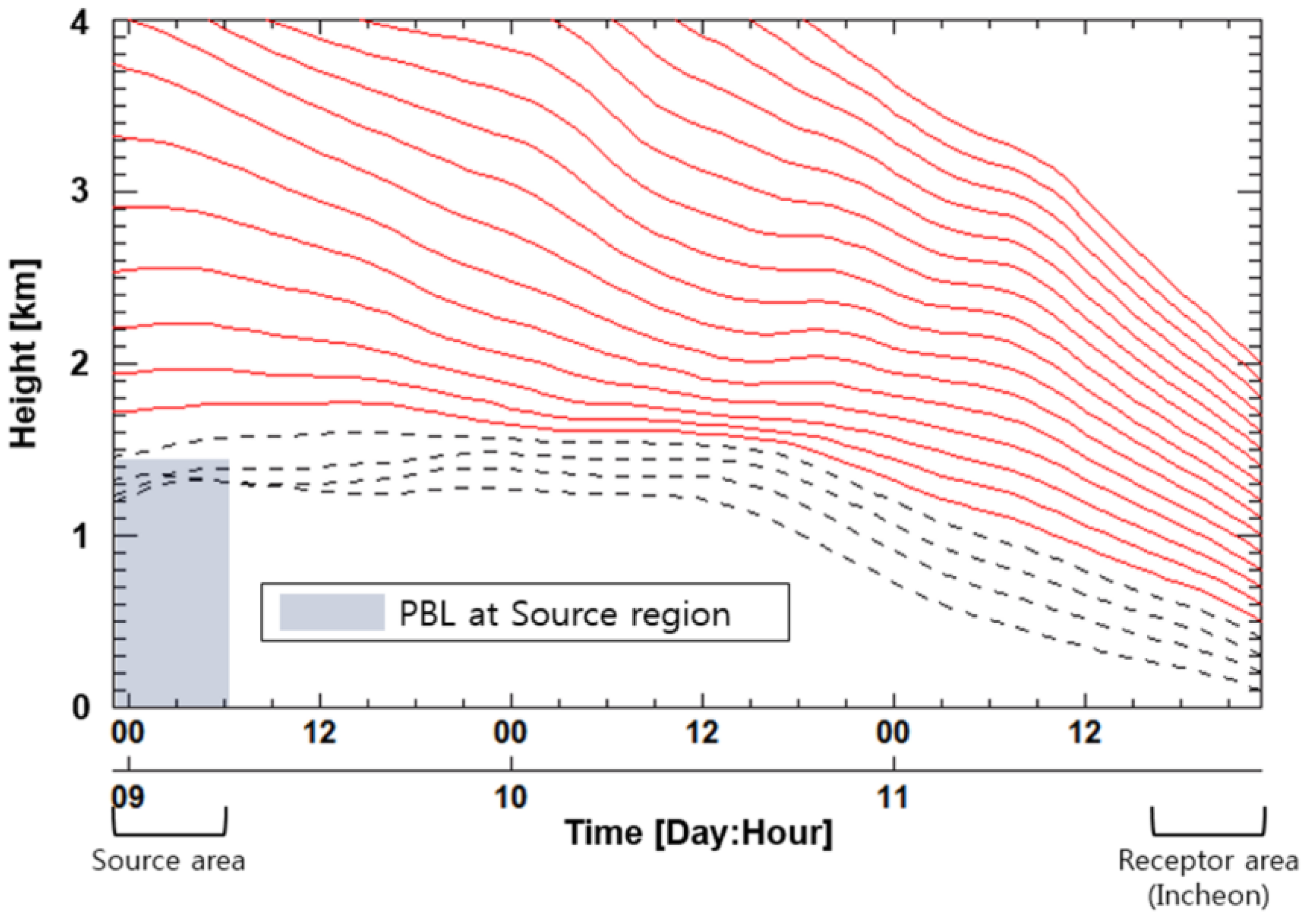
2.2. HYSPLIT Backward Trajectory Simulation

Three-day backward trajectories from the receptor sites (Seoul, Incheon, Gangneung, and Wonju) were calculated every hour at intervals of 0.1 km above ground level using the HYSPLIT model version 4.9 developed by the National Oceanic and Atmospheric Administration, Air Resources Laboratory (NOAA/ARL) [29]. Re-analysis meteorological data from the National Centers for Environmental Prediction/National Center for Atmospheric Research (NCEP/NCAR) were used for the trajectory calculation. The global reanalysis data are available on a 2.5° grid at 6 h intervals (synoptic times) on pressure surfaces. HYSPLIT backward trajectory simulations were conducted for the calculation of average air mass transportation speed between source and receptor areas. The calculation of average air mass transportation speed is described in Section 3.2. Uncertainties in the trajectory endpoints have been reported to be ~20% of the travel distance [30]. A more recent study of biases in backward trajectories reported that the errors in single trajectories may, in fact, be greater than 20%, especially if the error is in the first few time steps [31].

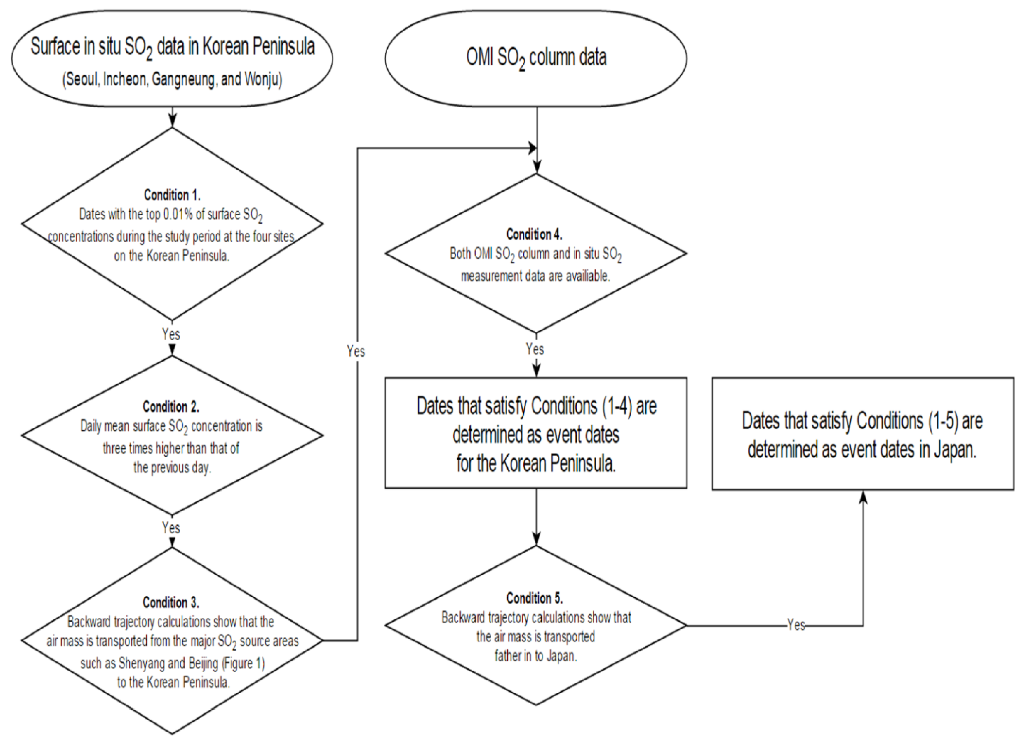
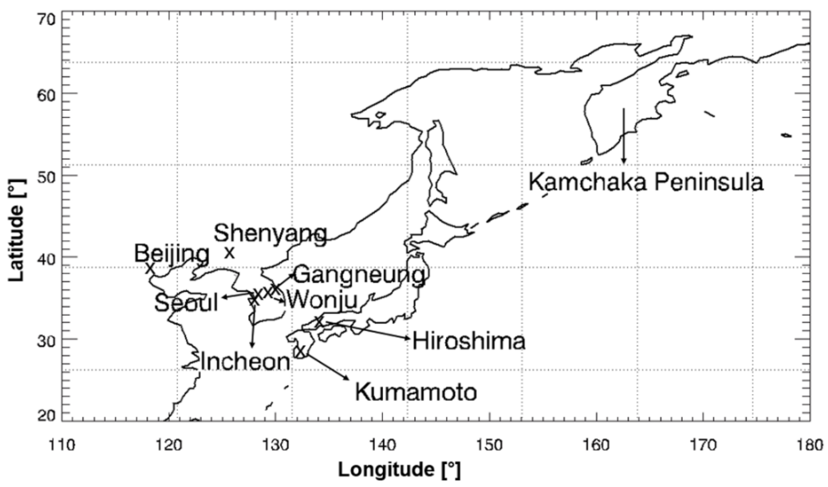
2.3. Study Locations and Dates

The flow rates of the LRT-SO2 were calculated for LRT-SO2 event dates. We define LRT-SO2 event dates as those when the SO2 at receptor sites is greatly enhanced by SO2 long-range transported from continental Asia. The flowchart in Figure 2 is used to determine LRT-SO2 events on the Korean Peninsula and Japan. Continuously monitored SO2 data are useful in quantifying the background SO2 level and are necessary to determine the LRT-SO2 event since the difference between the background SO2 level and the increase in SO2 level due to the LRT event at a receptor area is required. Therefore, we used in situ measurement data, which provide high continuity of surface SO2 data, together with OMI data to determine LRT-SO2 events as shown in Figure 2.
The following conditions (Figure 2) are applied in sequence to determine the dates of LRT-SO2 events when the contribution of LRT-SO2 from continental Asia to a receptor area is considered significant.
Condition 1. Dates with the top 0.01% of surface SO2 concentrations during the study period at the four sites on the Korean Peninsula.
Condition 2. Daily mean surface SO2 concentration is three times higher than that of the previous day.
Condition 3. Backward trajectory calculations show that the air mass is transported from the major SO2 source areas such as Shenyang and Beijing (Figure 1) to the Korean Peninsula.
Condition 4. Both OMI SO2 column and in situ SO2 measurement data are available. Dates that satisfy Conditions (1–4) are determined as event dates for the Korean Peninsula.
Condition 5. Backward trajectory calculations show that the air mass is transported farther into Japan. Dates that satisfy Conditions (1–5) are determined as event dates in Japan.
If SO2 concentration rapidly and significantly increases for a short time interval at the receptor sites, LRT-SO2 event is very likely to take place due to the almost negligible SO2 emission in Korean Peninsula in comparison with that at upwind regions [11]. Thus, Conditions 1 and 2 are applied to ensure the both rapid and significant increase in SO2 concentration for a short time interval at the receptor sites.
A low threshold value in Condition 1 allows dates with high surface SO2 concentration and also possibly high OMI SO2 column. On those dates, there can be larger differences between LRT-SO2 level and background SO2 level, which is controlled by local SO2 emission, than that on dates with low surface SO2 concentration (See Section 3.1 for the detailed description of the background SO2 level calculation). For example, on the dates that satisfy Condition 1 with the threshold of 0.05% instead of 0.01%, the average in situ mixing ratio and OMI SO2 column are 8 ppbv and 0.011 g·m−2, respectively. The OMI SO2 column of 0.011 g·m−2 is smaller than 0.016 g·m−2, the sum of background OMI SO2 level (0.004 g·m−2) and its uncertainty. The uncertainty of background OMI SO2 column in this present study is the sum of 0.001 g·m−2, the standard deviation of the background SO2 and 0.011 g·m−2, 1σ error of OMI SO2 column according to the literature [11]. Thus, there can be a large uncertainty in quantifying LRT-SO2. In the case of Condition 1 with the threshold 0.03%, the OMI SO2 column of 0.018 g·m−2 is slightly larger but still similar to 0.016 g·m−2, the sum of background OMI SO2 level and its uncertainty. In the case of Condition 1 with the threshold 0.01%, the OMI SO2 column of 0.033 g·m−2 is about two times larger than 0.016 g·m−2, the sum of background OMI SO2 level and its uncertainty, which is likely to lead to a smaller uncertainty in quantifying LRT-SO2 than that of using higher threshold values in Condition 1.
Table 1 lists the LRT-SO2 event dates determined using the five conditions shown in Figure 2. E1 through E7 represent high SO2 events when LRT-SO2 reaches the Korean Peninsula, whereas E8 and E9 refer to the events when LRT-SO2 reaches Japan via the Korean Peninsula. E10 and E11 did not meet the above five conditions, which require the surface SO2 in situ data since air mass pathways from the source areas do not pass over the Korean Peninsula where the surface SO2 in situ data are available. However, E10 and E11 were considered as LRT-SO2 events in the Northwest Pacific Ocean according to Hsu et al. [19], who reported events in which LRT-SO2 from continental Asia reached the Northwest Pacific Ocean using both OMI data and a transport model (HYSPLIT).

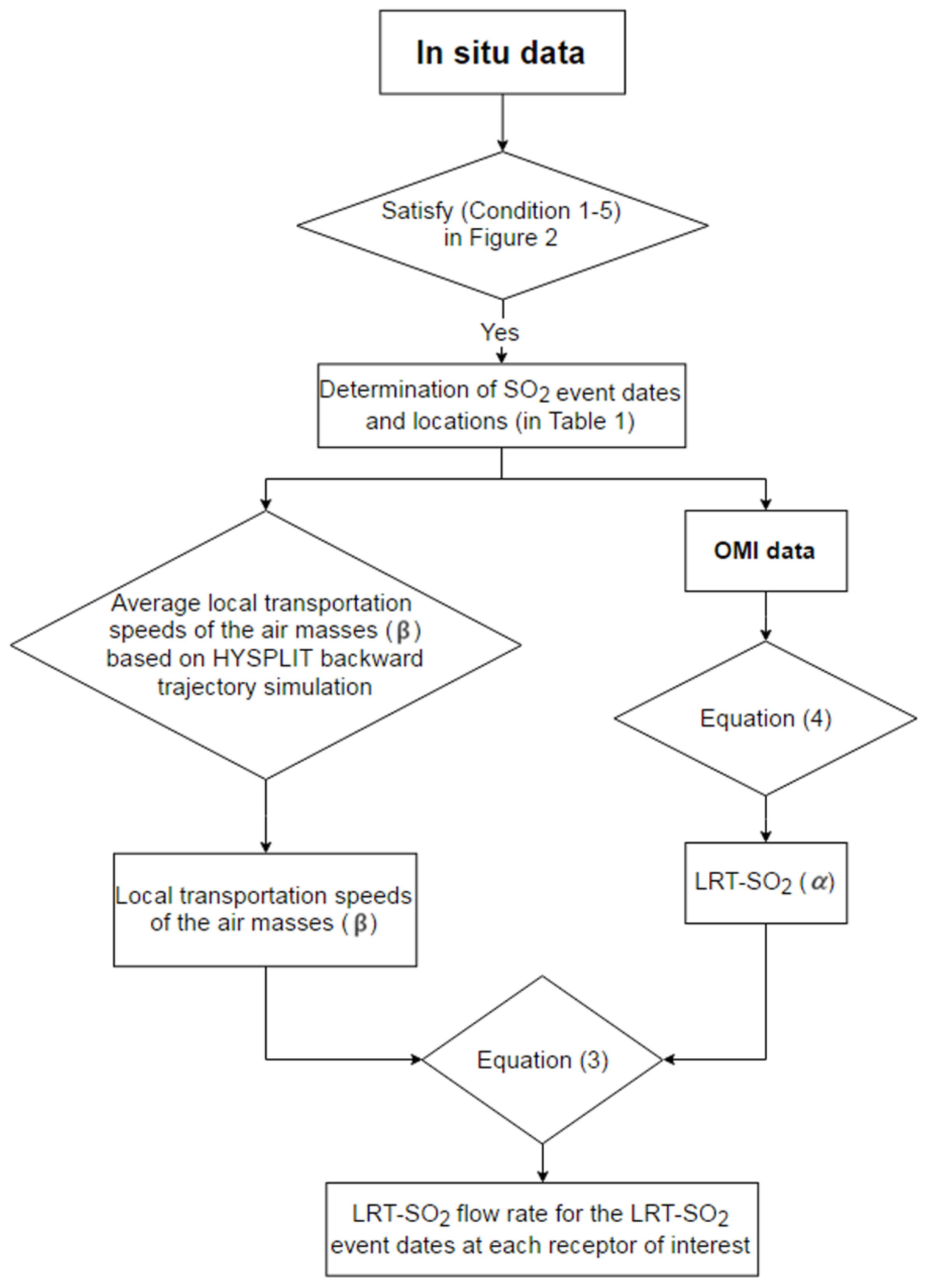
3. Flow Rate Calculation

Figure 3 summarizes the flow rate calculation for the LRT-SO2 event dates at each receptor location of interest. The LRT-SO2 flow rate in the present study represents the total mass of SO2 transported from continental Asia into the atmosphere over a receptor area of size equal to an OMI grid length per unit time. The LRT-SO2 flow rate can be expressed in terms of the average flux and cross-sectional area:
Flow rate   ( Mg · h 1   OMI · gird 1 )   =   average flux   ( Mg · km 2 · h 1 )   ×   cross-sectional area   ( km 2 )
The cross-sectional area in Equation (1) can be defined as the total cross-sectional area of the atmosphere that the long-range transported air mass flows through at a receptor area, and is located perpendicular to the long-range transported air mass transport direction at the receptor area. In the present study, the cross-sectional area is obtained by multiplying the OMI grid length by the atmospheric thickness. Atmospheric thickness is the distance between the surface and the Top Of the Atmosphere (TOA). The term “atmospheric thickness” eventually has no effect on the flow rate estimation since it is canceled out in Equation (3). The average flux term can be expressed as follows:
Average flux   ( Mg · km 2 · h 1 ) =   α   ( Mg · km 2 ) atmospheric thickness   ( km )   ×   β   ( km · h 1 )
Here, α denotes the LRT-SO2 column. LRT-SO2 column ( α ) means the SO2 column at a receptor area due to LRT from continental Asia. β denotes the average transportation speed of air mass. The transportation speed of air mass ( β ) can be defined as the average local transportation speeds of the air masses, which are originated within the PBL in a source area and are also within the OMI grid at a receptor site and the air mass here is assumed to contain SO2 that originates from the source region. Replacing the average flux term in Equation (1) with the terms on the right hand side of Equation (2), we have
SO 2   flow rate   ( Mg · h 1 OMI · gird 1 ) =   α   ( Mg · km 2 )   ×   β   ( km · h 1 )   ×   OMI grid length   ( km )
The OMI grid length is 25 km, since OMI Level 3 data were used in this study. The methods used to obtain the α and β are described in Section 3.1 and Section 3.2, respectively.

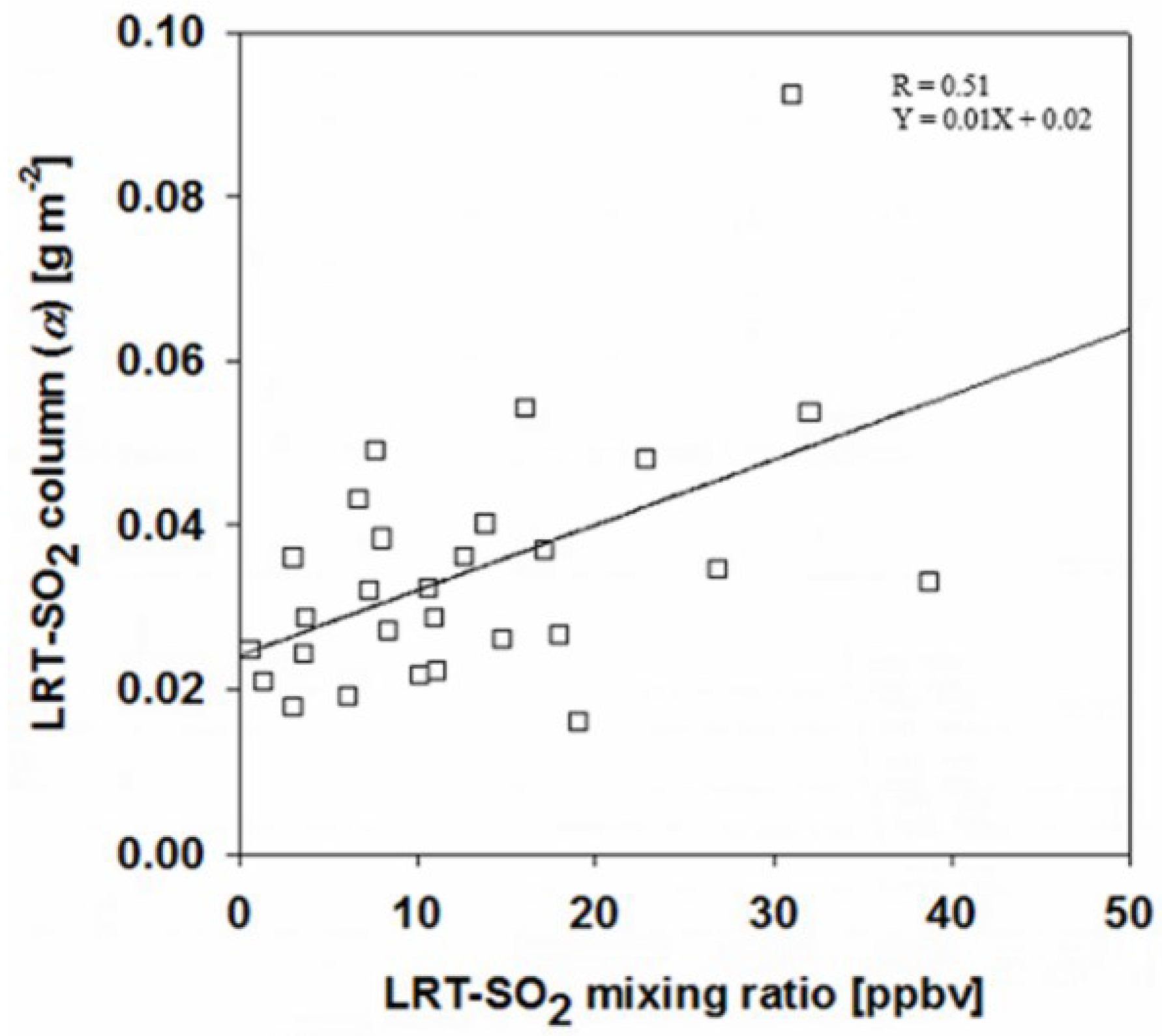
3.1. Calculation of α

α was calculated as follows:
α   = SO 2 VCD event SO 2 VCD local
In Equation (4), SO2 VCDlocal represents the SO2 vertical column density (VCD) due to local SO2 emission at a receptor area at an OMI overpass time for each event in Table 1. SO2 VCDlocal was calculated by averaging OMI SO2 column data that were available for the 15 days before and after each event date, excluding the data measured on the event date. SO2 VCDevent represents the OMI SO2 column measured for each event in Table 1. Table 2 lists the α values calculated for each event and receptor site. We found the mean value (0.033 g·m−2) of α to be much larger than 0.008 g·m−2, which is the sum of the mean SO2 VCDlocal (0.006 g·m−2) and the standard deviation of SO2 VCDlocal (0.001 g·m−2). This large α value, compared with SO2 VCDlocal plus its standard deviation, clearly distinguishes LRT-SO2 from local SO2. We also calculated LRT-surface SO2 mixing ratio using the Equation (4) but for surface mixing ratio instead of VCD. In Figure 4, LRT-SO2 mixing ratios were calculated using the in situ data averaged for a one-hour interval between 13:30 and 14:30 (LT). The α values are plotted against LRT-SO2 mixing ratios, showing certain agreement (R = 0.51) in Figure 4. The high R value between LRT-SO2 column and LRT-SO2 mixing ratio implies that the contribution of long-range transported SO2 to a receptor area is vertically similar, whereas the low R value means that the contribution of long-range transported SO2 to a receptor area is vertically different. The slope and intercept of the regression equation in Figure 4 do not mean much in comparison with the R value. However, there exists the y-interceptor (0.02) of the regression equation in Figure 4 due to no zero values present at x- and y-axis because only the data for the SO2 event periods can be used to calculate either LRT-SO2 column or LRT-SO2 mixing ratio in this present study.

3.2. Calculation of β

Sulfur dioxide is likely to be concentrated within the PBL at the source area. Therefore, the air mass that starts traveling within the PBL over continental Asia during the event in Table 1 is assumed to contain SO2 from the source area. We used the seasonal mean PBL height information reported by von Engeln and Teixeira [32] in order to reflect seasonal PBL variations at the source region on continental Asia. Air mass backward trajectories from each receptor site were computed every 0.1 km above ground level (agl) for each event, using the HYSPLIT model. The source areas, which are identified in this present study, are coincident with the areas with high SO2 emission reported in the Asian emission inventory study [8,11,33] and also the receptor modeling study [18]. β was calculated by averaging the local transportation speeds of the air masses, which are originated within the PBL in a source area and are also within the OMI grid at a receptor site. Figure 5 shows an example of the vertical distribution of the backward trajectories that started traveling between continental Asia and Incheon on 11 February 2006. Table 2 lists the β values for each event and receptor site as well as the LRT-SO2 flow rates for each event and receptor site using Equation (3) with the α and β values in Table 2.

4. Results

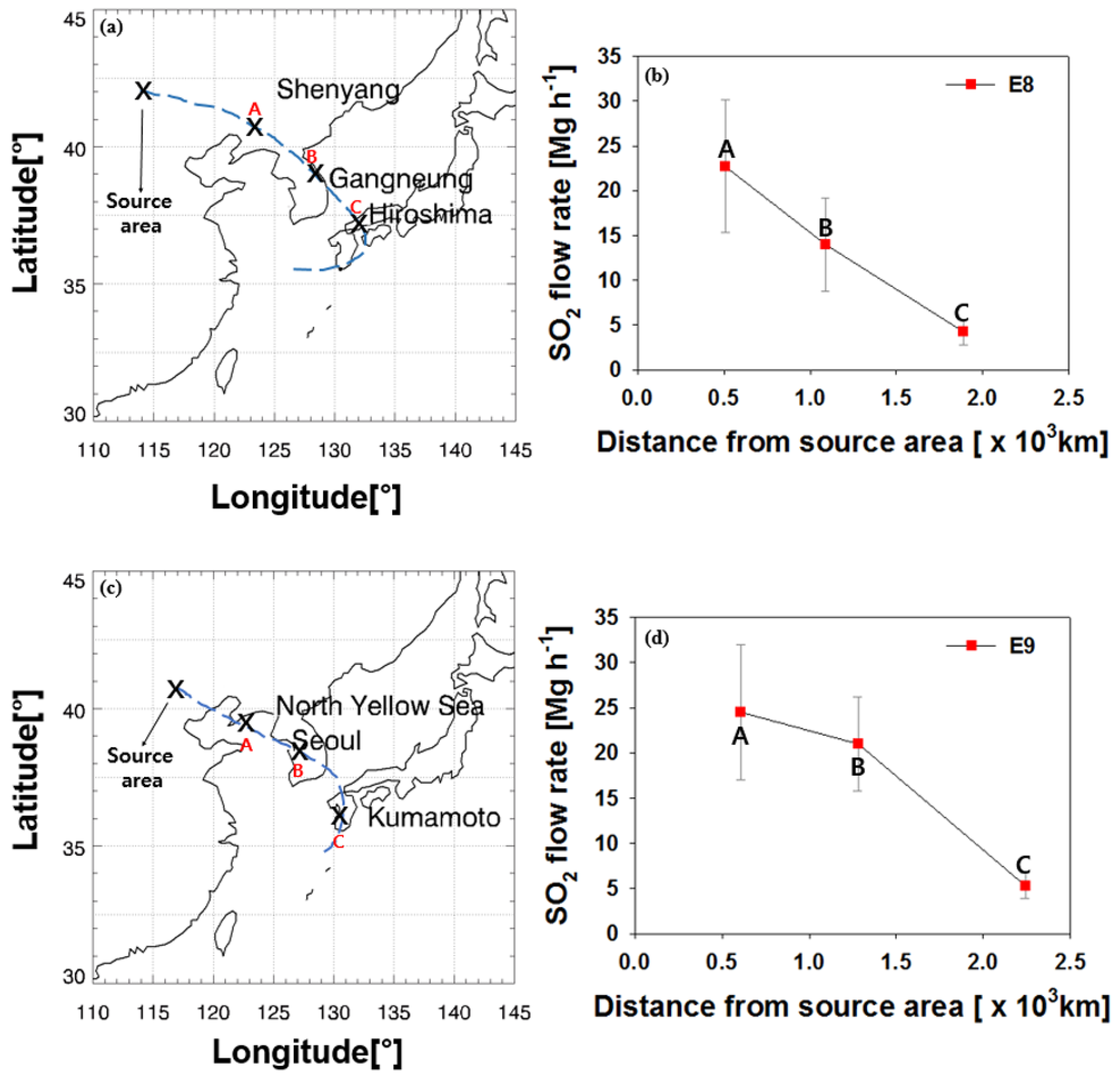
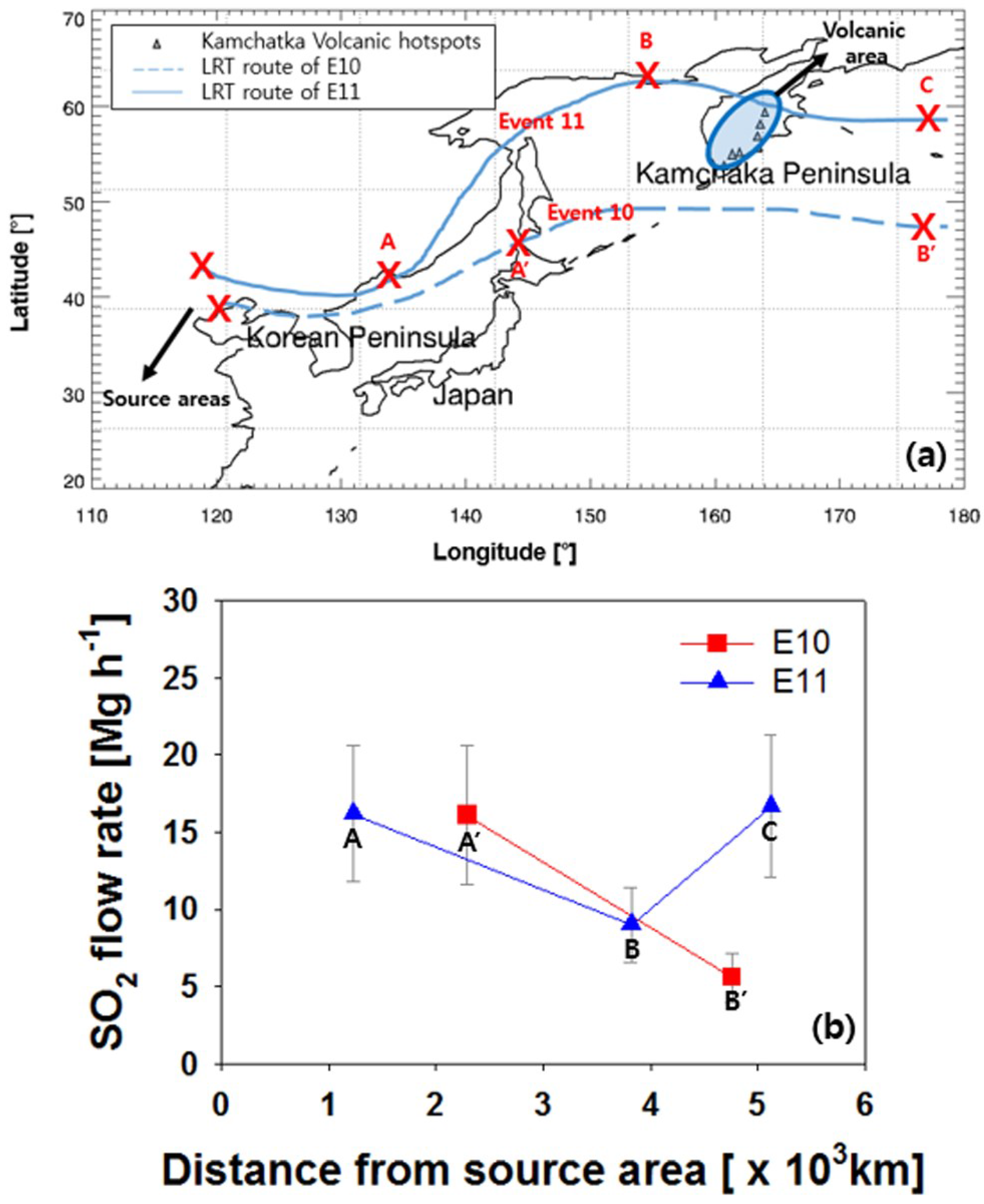
4.1. LRT-SO2 Flow Rates

Table 2 lists α and β, and LRT-SO2 flow rate for each event over the Korean Peninsula, Japan, and the Northwest Pacific Ocean. In events E1–E7, when LRT-SO2 reached the Korean Peninsula, the maximum flow rate is 33.4 Mg·h−1 OMI·gird−1 in Wonju on 22 December 2006, while the minimum flow rate is 2.9 Mg·h−1 OMI·gird−1 in Wonju on 8 November 2007. In events E8 and E9 when LRT-SO2 reaches Japan via the Korean Peninsula, the maximum flow rate is 24.5 Mg·h−1 OMI·gird−1 over the North Yellow Sea on 21 December 2006 while the minimum flow rate is 4.2 Mg·h−1 OMI·gird−1 at Hiroshima on 24 December 2006. In events E10 and E11, when LRT-SO2 reaches the Northwest Pacific Ocean, the maximum flow rate is 16.7 Mg·h−1 OMI·gird−1 at the Northwest Pacific Ocean (Bering Sea) Hokkaido 11 October 2006 whereas the minimum flow rate is 5.6 Mg·h−1 OMI·gird−1 at the Northwest Pacific Ocean (Aleutian islands) on 7 October 2008. A general decrease in LRT-SO2 flow rates with increasing distance from continental Asia can be associated with reduction in either α or β according to Equation (3). As shown in Table 2, the decreasing tendency in LRT-SO2 flow rate over transport distance is mostly due to a decreasing trend of α since β does not show any trend. The decreasing trend of α could be attributed to dispersion of SO2 over transport distance between a source area and a receptor area. In Table 2, average LRT-SO2 flow rates over the Korean Peninsula, Japan, and the Northwest Pacific Ocean are calculated to be 13.1, 8.5, and 11.2 Mg·h−1 OMI·gird−1, respectively. We have the average flow rate over the Northwest Pacific Ocean higher than that over Japan due to the contribution of the volcanic emissions, which are explained in detail later in this section.
We investigated the variations in LRT-SO2 flow rates as a function of distance from continental Asia for events E8–E11. Figure 6a shows the backward trajectories that correspond to events E8 in Table 1, while Figure 6b shows the variation of the LRT-SO2 flow rate for event E8 as a function of distance from continental Asia. In Figure 6a, A, B, and C represent the locations of the air mass backward trajectory for event E8 on 22–24 December 2006 at Shenyang, Gangneung, and Hiroshima, respectively. The corresponding SO2 flow rates, shown in Figure 6b, have values of 22.7, 14.0, and 4.2 Mg·h−1 OMI·gird−1 at A, B, and C, which are 510, 1090, and 1890 km from the source area, respectively. Figure 6c,d is the same as Figure 6a,b but for E9. In Figure 6c, A, B, and C represent the locations of the air mass backward trajectories for event E9 on 21–23 December 2006 over the North Yellow Sea, Seoul, and Kagoshima, respectively. The corresponding SO2 flow rates for E9, shown in Figure 6d, have values of 24.5, 21.0, and 5.3 Mg·h−1 OMI·gird−1 at A, B, and C, which are 610, 1280, and 2240 km from the source area, respectively. Although the distances between the receptor locations (B and C) and the source area for event E8 in Figure 6a,b are slightly different from those for event in Figure 6c,d, we found that the LRT-SO2 flow rates at receptor sites B and C in Figure 6b are closely similar to those for B and C in Figure 6d. The similarity between the LRT-SO2 flow rates in Figure 6b,d may be associated with the similarity between the two event periods in December 2006 as well as between the air mass pathways for events E8 and E9. The rate of decrease in the LRT-SO2 flow rate between locations A and C is 13.4 Mg·h−1 OMI·gird−1 per 1000 km distance from the source area in Figure 6b compared with 11.8 Mg·h−1 OMI·gird−1 per 1000 km distance from the source area in Figure 6d.
Figure 7a shows the backward trajectories that correspond to events E10 and E11 in Table 1, while Figure 7b shows the variation of the LRT-SO2 flow rate for events E10 and E11 as a function of distance from continental Asia. In Figure 7a, A’ and B’ represent the locations of the air mass backward trajectory for event E10 on 6–7 October 2008 at Hokkaido and the Northwest Pacific Ocean (Aleutian Islands), respectively, and A, B, and C represent those for event E11 on 9–11 October 2006 at Vladivostok, Magadan, and the Northwest Pacific Ocean (Bering Sea), respectively. The corresponding LRT-SO2 flow rates are shown in Figure 7b. The values for event E10 are calculated to be 16.1 and 5.6 Mg·h−1 OMI·gird−1 at A’ and B’, which are 2290 and 4760 km from the source area, respectively. The values for event E11 are 16.2, 9.0, and 16.7 Mg·h−1 OMI·gird−1 at A, B, and C, which are 1230, 3820, and 5120 km from the source area, respectively. We found a general decrease in LRT-SO2 flow rates with distance from the source region except for locations between B and C. The increase in LRT-SO2 between B and C in Figure 7b could be attributed to the contribution of SO2 from continuous volcanic emissions (e.g., Sheveluch, Klyuchevskov, Bezymianny, Karymsky, Ebeko, Severgin, and Berga) over the Kamchatka Peninsula, which is located on the air mass pathway between B and C in Figure 7a. The increase in LRT-SO2 between B and C in Figure 7b is thought to be associated with the contribution of the volcanic emissions since the volcanic gas emissions except for large eruption cases are generally known to affect the lower troposphere [34,35,36,37]. The rate of decrease in the LRT-SO2 flow rate between locations A’ and B’ is 4.3 Mg·h−1 OMI·gird−1 per 1000 km distance from the source area for event E10, whereas that between locations A and B is 4.5 Mg·h−1 OMI·gird−1 per 1000 km distance from the source area for event E11.

4.2. Error Estimation

The uncertainties in LRT-SO2 flow rate were calculated following the error propagation analysis of Clifford [38]:
σ =   flow rate 2 × ( ( σ α α ) 2 + ( σ β β ) 2 )
Here, flow rate represents the LRT-SO2 flow rate. σ represents the uncertainty in LRT-SO2 flow rate, and σ α and σ β represent the uncertainties in α and β , respectively. In this present study, OMI SO2 column uncertainty of 45% was used for σ α following Lee at el. [39]. We also calculated σ β , which is composed of the covariance of the distance and time for each trajectory as well as the uncertainty in air mass transportation speed. We used 20% for the uncertainty in air mass transportation speed, following Stohl [30]. The LRT-SO2 flow rate uncertainties calculated using Equation (5) are shown as numbers in brackets in Table 2. The uncertainties are also indicated by the error bars in Figure 6b,d and Figure 7b. For all events from E1 through E11, the uncertainties in LRT-SO2 flow rate range from 51% to 61% (average, 56%).

5. Conclusions

We report the first use of the OMI SO2 column and backward trajectory simulation to calculate the LRT-SO2 flow rate from continental Asia to the Korean Peninsula, Japan, and the Northwest Pacific Ocean. In general, we found a decreasing trend in LRT-SO2 flow rates with distance from the source region. However, the flow rate increased with distance from continental Asia in the case of event E11 when large volcanic areas in the Kamchatka Peninsula, another significant SO2 source, are located on the air mass pathway between continental Asia and the Northwest Pacific Ocean (Bering Sea). For future studies, the method for estimation of LRT-SO2 can be applied to other downwind regions with significant SO2 emission sources. The method can also be utilized for other atmospheric species (e.g., CO and aerosol). As the information of a transported air pollutant amount can be available at a receptor area, this method is expected to be useful for the efficient local air quality management. In addition, the application of this method to geostationary measurements (e.g., Geostationary Environmental Monitoring Spectrometer (GEMS)) allows quantifying the hourly amount of gases or aerosols that are long-range transported from a source area to receptor areas.

Acknowledgments

This work was funded by the Korea Meteorological Administration Research and Development Program under Grant KMIPA 2015-6030, Korea. The authors acknowledge the NOAA Air Resources Laboratory (ARL) for providing HYSPLIT model backward trajectory data, the National Institute of Environmental Research (NIER) for providing SO2 mixing ratio data, and NASA for providing SO2 Planetary Boundary Layer (PBL) column density data.

Author Contributions

Junsung Park carried out the flow rate calculations; Hanlim Lee performed HYSPLIT backward trajectory simulations and Ozone Monitoring Instrument (OMI) retrievals; Jaeyong Ryu carried out in situ measurements.

Conflicts of Interest

The authors declare no conflict of interest.

Abbreviations

The following abbreviations are used in this manuscript:
OMI
Ozone Monitoring Instrument
MAX-DOAS
Multi AXis Differential Optical Absorption Spectroscopy
CPSCF
Conditional Potential Source Contribution Function
GEO
GEostationary Orbit
LEO
Low Earth Orbit
TOA
Top Of the Atmosphere
Agl
Above ground level
CALIPSO
Cloud-Aerosol Lidar and Infrared Pathfinder Satellite Observations
SCIAMACHY
SCanning Imaging Absorption SpectroMeter for Atmospheric CHartographY
HYSPLIT
HYbrid Single Particle Lagrangian Integrated Trajectory
MODIS
MODerate resolution Imaging Spectroradiometer
MISR
Multi-angle Imaging SpectroRadiometer

References

  1. Weiss, K.; Gergen, P.J.; Wagener, D.K. Breathing better or wheezing worse? The changing epidemiolgy of asthma morbidity and mortality. Annu. Rev. Public Health 1993, 14, 491–513. [Google Scholar] [CrossRef] [PubMed]
  2. Dockery, D.W.; Cunningham, J.; Damokosh, A.I.; Neas, L.M.; Spengler, J.D.; Koutrakis, P.; Ware, J.H.; Raizenne, M.; Speizer, F.E. Health effects of acid aerosols on North American children: Respiratory symptoms. Environ. Health Perspect. 1996, 104, 500–505. [Google Scholar] [CrossRef] [PubMed]
  3. Sunyer, J.; Spix, C.; Quenel, P.; Ponce-de-Leon, A.; Pönka, A.; Barumandzadeh, T.; Touloumi, G.; Bacharova, L.; Wojtyniak, B.; Vonk, J.; et al. Urban air pollution and emergency admissions for asthma in four European cities: The aphea project. Thorax 1997, 52, 760–765. [Google Scholar] [CrossRef] [PubMed]
  4. Thompson, A.J.; Shields, M.D.; Patterson, C.C. Acute asthma exacerbations and air pollutants in children living in belfast, Northern Ireland. Arch. Environ. Health Int. J. 2001, 56, 234–241. [Google Scholar] [CrossRef] [PubMed]
  5. Seinfeld, J.H.; Pandis, S.N. Atmospheric Chemistry and Physics; Wiley-Interscience: Hoboken, NJ, USA, 2006. [Google Scholar]
  6. Whelpdale, D.M.; Watch, G.A.; Kaiser, M. Global Acid Deposition Assessment; World Meteorological Organization, Global Atmosphere Watch: Geneva, Switzerland, 1996. [Google Scholar]
  7. Vestreng, V.; Myhre, G.; Fagerli, H.; Reis, S.; Tarrasón, L. Twenty-five years of continuous sulphur dioxide emission reduction in Europe. Atmos. Chem. Phys. 2007, 7, 3663–3681. [Google Scholar] [CrossRef]
  8. Lu, Z.; Streets, D.G.; Zhang, Q.; Wang, S.; Carmichael, G.R.; Cheng, Y.F.; Wei, C.; Chin, M.; Diehl, T.; Tan, Q. Sulfur dioxide emissions in China and sulfur trends in East Asia since 2000. Atmos. Chem. Phys. 2010, 10, 6311–6331. [Google Scholar] [CrossRef]
  9. Jiang, J.; Zha, Y.; Gao, J.; Jiang, J. Monitoring of SO2 column concentration change over China from Aura OMI data. Int. J. Remote Sens. 2012, 33, 1934–1942. [Google Scholar] [CrossRef]
  10. Krotkov, N.; McLinden, C.; Li, C.; Lamsal, L.; Celarier, E.; Marchenko, S.; Swartz, W.; Bucsela, E.; Joiner, J.; Duncan, B.; et al. Aura OMI observations of regional SO2 and NO2 pollution changes from 2005 to 2014. Atmos. Chem. Phys. Discuss. 2015, 15, 26555–26607. [Google Scholar] [CrossRef]
  11. Kurokawa, J.; Ohara, T.; Morikawa, T.; Hanayama, S.; Janssens-Maenhout, G.; Fukui, T.; Kawashima, K.; Akimoto, H. Emissions of air pollutants and greenhouse gases over Asian regions during 2000–2008: Regional emission inventory in Asia (REAS) version 2. Atmos. Chem. Phys. 2013, 13, 11019–11058. [Google Scholar] [CrossRef]
  12. Park, R.J.; Jacob, D.J.; Field, B.D.; Yantosca, R.M.; Chin, M. Natural and transboundary pollution influences on sulfate-nitrate-ammonium aerosols in the United States: Implications for policy. J. Geophys. Res. Atmos. 2004, 109. [Google Scholar] [CrossRef]
  13. Heald, C.L.; Jacob, D.J.; Park, R.J.; Alexander, B.; Fairlie, T.D.; Yantosca, R.M.; Chu, D.A. Transpacific transport of Asian anthropogenic aerosols and its impact on surface air quality in the United States. J. Geophys. Res. Atmos. 2006, 111. [Google Scholar] [CrossRef]
  14. Donkelaar, A.V.; Martin, R.V.; Leaitch, W.R.; Macdonald, A.; Walker, T.; Streets, D.G.; Zhang, Q.; Dunlea, E.J.; Jimenez, J.L.; Dibb, J.E.; et al. Analysis of aircraft and satellite measurements from the intercontinental chemical transport experiment (INTEX-B) to quantify long-range transport of East Asian sulfur to Canada. Atmos. Chem. Phys. 2008, 8, 2999–3014. [Google Scholar] [CrossRef]
  15. Haywood, J.; Shine, K. The effect of anthropogenic sulfate and soot aerosol on the clear sky planetary radiation budget. Geophys. Res. Lett. 1995, 22, 603–606. [Google Scholar] [CrossRef]
  16. Lee, C.; Richter, A.; Lee, H.; Kim, Y.J.; Burrows, J.P.; Lee, Y.G.; Choi, B.C. Impact of transport of sulfur dioxide from the Asian continent on the air quality over Korea during may 2005. Atmos. Environ. 2008, 42, 1461–1475. [Google Scholar] [CrossRef]
  17. Dickerson, R.; Li, C.; Li, Z.; Marufu, L.; Stehr, J.; McClure, B.; Krotkov, N.; Chen, H.; Wang, P.; Xia, X.; et al. Aircraft observations of dust and pollutants over Northeast China: Insight into the meteorological mechanisms of transport. J. Geophys. Res. Atmos. 2007, 112. [Google Scholar] [CrossRef]
  18. Jeong, U.; Lee, H.; Kim, J.; Kim, W.; Hong, H.; Song, C.K. Determination of the inter-annual and spatial characteristics of the contribution of long-range transport to SO2 levels in Seoul between 2001 and 2010 based on conditional potential source contribution function (CPSCF). Atmos. Environ. 2013, 70, 307–317. [Google Scholar] [CrossRef]
  19. Hsu, N.C.; Li, C.; Krotkov, N.A.; Liang, Q.; Yang, K.; Tsay, S.C. Rapid transpacific transport in autumn observed by the A-TRAIN satellites. J. Geophys. Res. Atmos. 2012, 117. [Google Scholar] [CrossRef]
  20. Mallik, C.; Lal, S.; Naja, M.; Chand, D.; Venkataramani, S.; Joshi, H.; Pant, P. Enhanced SO2 concentrations observed over Northern India: Role of long-range transport. Int. J. Remote Sens. 2013, 34, 2749–2762. [Google Scholar] [CrossRef]
  21. Li, C.; Krotkov, N.A.; Dickerson, R.R.; Li, Z.; Yang, K.; Chin, M. Transport and evolution of a pollution plume from Northern China: A satellite-based case study. J. Geophys. Res. Atmos. 2010, 115. [Google Scholar] [CrossRef]
  22. Levelt, P.F.; Van den Oord, G.H.; Dobber, M.R.; Malkki, A.; Visser, H.; De Vries, J.; Stammes, P.; Lundell, J.O.; Saari, H. The ozone monitoring instrument. IEEE Trans. Geosci. Remote Sens. 2006, 44, 1093–1101. [Google Scholar] [CrossRef]
  23. Krotkov, N.; Yang, K.; Carn, S.; Krueger, A. OMSO2 README File Date: 2/26/2008; NASA: Greenbelt, MD, USA, 2006.
  24. Krotkov, N.A.; Carn, S.A.; Krueger, A.J.; Bhartia, P.K.; Yang, K. Band residual difference algorithm for retrieval of SO2 from the Aura ozone monitoring instrument (OMI). IEEE Trans. Geosci. Remote Sens. 2006, 44, 1259–1266. [Google Scholar] [CrossRef]
  25. Goddard Earth Sciences Data and Information Services Center (GES-DISC). Available online: http://disc.sci.gsfc.nasa.gov/Aura/data-holdings/OMI/omso2e_v003.html (accessed on 6 April 2016).
  26. Li, C.; Joiner, J.; Krotkov, N.A.; Bhartia, P.K. A fast and sensitive new satellite SO2 retrieval algorithm based on principal component analysis: Application to the ozone monitoring instrument. Geophys. Res. Lett. 2013, 40, 6314–6318. [Google Scholar] [CrossRef]
  27. Ozone Monitoring Instrument Data User’s Guide. Available online: http://disc.sci.gsfc.nasa.gov/Aura/additional/documentation/README.OMI_DUG.pdf (accessed on 6 April 2016).
  28. Goddard Earth Sciences Data and Information Services Center (GES-DISC). Available online: http://disc.sci.gsfc.nasa.gov/Aura/data-holdings/OMI/index.shtml#info (accessed on 6 April 2016).
  29. Draxler, R.R.; Hess, G. Description of the HYSPLIT4 Modeling System; NOAA Air Resources Laboratory: Silver Spring, MD, USA, 1997.
  30. Stohl, A. Computation, accuracy and applications of trajectories—A review and bibliography. Atmos. Environ. 1998, 32, 947–966. [Google Scholar] [CrossRef]
  31. Gebhart, K.A.; Schichtel, B.A.; Barna, M.G. Directional biases in back trajectories caused by model and input data. J. Air Waste Manag. Assoc. 2005, 55, 1649–1662. [Google Scholar] [CrossRef] [PubMed]
  32. Von Engeln, A.; Teixeira, J. A planetary boundary layer height climatology derived from ECMWF reanalysis data. J. Clim. 2013, 26, 6575–6590. [Google Scholar] [CrossRef]
  33. Zhang, X.; Geffen, J.; Zhang, P.; Wang, J. Trend spatial & temporal distribution, and sources of the tropospheric SO2 over China based on satellite measurement during 2004–2009. Proc. Dragon 2010, 2, 2008–2010. [Google Scholar]
  34. Lee, H.-L.; Kim, J.-H.; Ryu, J.-Y.; Kwon, S.-C.; Noh, Y.-M.; Gu, M.-J. 2-Dimensional mapping of sulfur dioxide and bromine oxide at the sakurajima volcano with a ground based scanning imaging spectrograph system. J. Opt. Soc. Korea 2010, 14, 204–208. [Google Scholar] [CrossRef]
  35. Lee, C.; Kim, Y.J.; Tanimoto, H.; Bobrowski, N.; Platt, U.; Mori, T.; Yamamoto, K.; Hong, C.S. High CLO and ozone depletion observed in the plume of sakurajima volcano, Japan. Geophys. Res. Lett. 2005, 32. [Google Scholar] [CrossRef]
  36. Bobrowski, N.; Hönninger, G.; Galle, B.; Platt, U. Detection of bromine monoxide in a volcanic plume. Nature 2003, 423, 273–276. [Google Scholar] [CrossRef] [PubMed]
  37. Bobrowski, N.; Von Glasow, R.; Aiuppa, A.; Inguaggiato, S.; Louban, I.; Ibrahim, O.; Platt, U. Reactive halogen chemistry in volcanic plumes. J. Geophys. Res. Atmos. 2007, 112. [Google Scholar] [CrossRef]
  38. Clifford, A. Multivariate Error Analysis: A Handbook of Error Propagation and Calculation in Many-Parameter System; Applied Science Publishers Ltd.: London, UK, 1973. [Google Scholar]
  39. Lee, C.; Martin, R.V.; van Donkelaar, A.; O’Byrne, G.; Krotkov, N.; Richter, A.; Huey, L.G.; Holloway, J.S. Retrieval of vertical columns of sulfur dioxide from SCIAMACHY and OMI: Air mass factor algorithm development, validation, and error analysis. J. Geophys. Res. Atmos. 2009, 114, D22303. [Google Scholar] [CrossRef]
Figure 1. Locations of SO2 source and receptor sites.
Atmosphere 07 00053 g001
Figure 2. Flowchart for the determination of high SO2 event dates over the Korean Peninsula and Japan.
Atmosphere 07 00053 g002
Figure 3. Flow rate of the calculation method for the LRT-SO2 event dates at each receptor location of interest.
Atmosphere 07 00053 g003
Figure 4. Correlations between LRT-SO2 column ( α ) and LRT-surface SO2 mixing ratio.
Atmosphere 07 00053 g004
Figure 5. Example of the vertical distribution of three-day HYSPLIT backward trajectories for air masses arriving in Incheon on 11 February 2006 (Local Time).
Atmosphere 07 00053 g005
Figure 6. (a) air mass pathways for event E8; (b) LRT-SO2 flow rate as a function of distance from the source area. A, B, and C in (a) and (b) correspond to Shenyang, Gangneung, and Hiroshima, respectively; (c) air mass pathways for event E9; (d) LRT-SO2 flow rate as a function of distance from the source area. A, B, and C in (c) and (d) correspond to the North Yellow Sea, Seoul, and Kumamoto, respectively.
Atmosphere 07 00053 g006
Figure 7. (a) air mass pathways for event E10 (dashed line) and E11 (solid line). Open triangles indicate Kamchatka volcanic hotspots. (b) SO2 flow rate as a function of distance from the source areas. A’ and B’ in (a) and (b) correspond to Hokkaido and the Northwest Pacific Ocean (Aleutian Islands), respectively. A, B, and C in (a) and (b) correspond to Vladivostok, Magadan, and the Northwest Pacific Ocean (Bering Sea), respectively.
Atmosphere 07 00053 g007
Table 1. LRT-SO2 events determined for each receptor area.
EventDateReceptor Area
E123 January 2005Seoul, Wonju
24 January 2005Seoul, Wonju
E211 February 2006Seoul, Incheon
E322 December 2006Seoul, Incheon, Wonju
23 December 2006Seoul, Incheon, Wonju
E413 March 2007Seoul, Incheon
14 March 2007Seoul, Incheon
15 March 2007Seoul, Incheon
E57 November 2007Seoul, Wonju
8 November 2007Seoul, Wonju
E611 March 2008Seoul, Wonju
E76 January 2008Incheon, Gangneung
7 January 2008Incheon, Gangneung
E822 December 2006Shenyang
23 December 2006Gangneung
24 December 2006Hiroshima
E921 December 2006North Yellow Sea
22 December 2006Seoul
23 December 2006Kumamoto
E106 October 2008Hokkaido
7 October 2008Northwest Pacific Ocean (Aleutian islands)
E119 October 2006Vladivostok
10 October 2006Magadan
11 October 2006Northwest Pacific Ocean (Bering Sea)
Table 2. Estimated LRT-SO2 flow rate and the parameters (α and β) used to estimate the long-range transported flow rate for each event.
Eventα a, α b, α c, α d (g·m−2)β a, β b, β c, β d (m·s−1)Flow Rate (Error) (Mg·h−1 OMI·grid−1)
E1230.036 a, 0.019 d3.0 a, 3.0 d9.7 a (±2.5), 5.1 d (±1.4)
240.038 a, 0.022 d5.1 a, 4.7 d17.4 a (±4.7), 9.3 d (±2.5)
E2110.049 a, 0.020 b6.3 a, 6.3 b27.8 a (±7.5), 11.3 b (±3.1)
E3220.036 a, 0.031 b, 0.054 d7.3 a, 7.2 b, 6.8 d23.7 a (±6.3), 20.0 b (±5.3), 33.4 d (±8.7)
230.024 a, 0.024 b,0.092 d4.1 a, 4.1 b, 3.8 d8.9 a (±2.4), 8.9 b (±2.4), 31.5 d (±8.3)
E4130.040 a, 0.027 b4.3 a, 4.1 b15.5 a (±4.1), 10.0 b (±2.7)
140.048 a, 0.040 b1.1 a, 1.1 b4.8 a (±1.3), 4.0 b (±1.1)
150.034 a, 0.025 b4.6 a, 4.8 b14.1 a (±3.8), 10.8 b (±3.0)
E570.029 a, 0.018 d3.3 a, 3.8 d8.6 a (±2.2), 6.2 d (±1.5)
80.027 a, 0.016 d1.5 a, 2.0 d3.6 a (±1.0), 2.9 d (±0.8)
E6110.033 a, 0.053 d3.7 a, 2.4 d11.0 a (±2.9), 11.4 d (±3.0)
E760.030 b, 0.021 c1.5 b, 2.7 c4.1 b (±1.1), 5.1 c (±1.4)
70.026 b, 0.035 c7.8 b, 8.6 c18.3 b (±4.8), 27.1 c (±7.0)
E8220.0357.222.7 (±7.4)
230.0334.714.0 (±3.7)
240.0133.64.2 (±1.2)
E9210.0475.824.5 (±7.5)
220.0327.321.0 (±5.2)
230.0105.95.3 (±1.4)
E1060.0286.416.1 (±4.5)
70.0193.35.6 (±1.6)
E1190.0345.316.2 (±4.4)
100.0205.09.0 (±2.4)
110.0257.416.7 (±4.6)
a Seoul; b Incheon; c Gangneung; d Wonju.

