
The Application of TAPM for Site Specific Wind Energy Forecasting

School of Photovoltaic and Renewable Energy Engineering, University of New South Wales, Sydney, NSW 2052, Australia
Atmosphere 2016, 7(2), 23; https://doi.org/10.3390/atmos7020023
Submission received: 6 December 2015
/
Revised: 25 January 2016
/
Accepted: 26 January 2016
/
Published: 5 February 2016
(This article belongs to the Special Issue Climate Variable Forecasting)
Abstract
:The energy industry uses weather forecasts for determining future electricity demand variations due to the impact of weather, e.g., temperature and precipitation. However, as a greater component of electricity generation comes from intermittent renewable sources such as wind and solar, weather forecasting techniques need to now also focus on predicting renewable energy supply, which means adapting our prediction models to these site specific resources. This work assesses the performance of The Air Pollution Model (TAPM), and demonstrates that significant improvements can be made to only wind speed forecasts from a mesoscale Numerical Weather Prediction (NWP) model. For this study, a wind farm site situated in North-west Tasmania, Australia was investigated. I present an analysis of the accuracy of hourly NWP and bias corrected wind speed forecasts over 12 months spanning 2005. This extensive time frame allows an in-depth analysis of various wind speed regimes of importance for wind-farm operation, as well as extreme weather risk scenarios. A further correction is made to the basic bias correction to improve the forecast accuracy further, that makes use of real-time wind-turbine data and a smoothing function to correct for timing-related issues. With full correction applied, a reduction in the error in the magnitude of the wind speed by as much as 50% for “hour ahead” forecasts specific to the wind-farm site has been obtained.
1. Introduction
Weather forecasting plays an important role within the electricity industry [1], with forecasts mainly focusing on estimating future demand, which is primarily temperature dependent. The inclusion of highly variable and somewhat unpredictable renewable energy sources such as wind into the generation mix poses new challenges for electricity industry operation, as the weather now has an impact on supply as well as demand. The wind energy sector has grown substantially over the past decade and is now emerging as an important contributor to electricity generation around the world [2,3,4]. Useful predictions of future wind output can play a valuable role in appropriately committing (starting) and dispatching other generation to meet expected demand. The number of research groups investigating how to better predict wind power due to the increased uptake of wind energy is also growing, as is the emergence of some commercial wind power forecast providers ([5,6,7,8,9,10], to name a few).
Providing wind farm specific forecasts has different challenges to conventional weather forecasts. From a meteorological perspective, a key challenge is one of scale. A wind farm requires accurate, near-real-time wind speed and direction forecasts for a specific height over a relatively small area. These site specific forecasts are often required for remote locations subject to highly variable conditions (e.g., coastal sites). The turbines on a wind farm also can span an area covering 5 km2 or greater depending on the size of the farm, with not all turbines experiencing the same wind regime due to effects of terrain, turbulence, and other turbines. Traditional numerical weather prediction (NWP) models have not been designed for forecasts at these scales.
Currently, three general approaches are taken in producing wind farm specific forecasts, with the choice dependent upon the forecast time horizon. The first approach is statistical in nature with techniques including time series models and Artificial Neural Networks (ANN) applied to historical site wind speed or power output data to provide forecasts from minutes to a few hours ahead [11,12,13,14]. The second approach is physical and involves designing new meso- and micro-scale NWPs devoted to providing local wind forecasts at typically hourly resolution for up to 72 h ahead. Usually this approach involves modifying an already existing NWP with some meso-scale development [15]. A problem arises here for short-term forecasting as once a NWP run has been initiated, the model is not as accurate in the first 6 h and these early results often need to be discarded. This is known as model spin-up [16]. The third approach is a combination of the two approaches above, and involves methods that combine existing NWP outputs with real-time local data and advanced statistical analyses to produce site-specific predictions [17,18,19,20,21].
In this paper, I concentrate on the third approach and show that by taking NWP outputs and applying a bias correction methodology improved predictions of wind speeds of importance to wind farm performance are obtained. The bias correction methodology has been applied to a range of weather conditions over the year and we show its successful use in predicting “fair weather” and an extreme weather event. The observational data from the wind farm site and forecast model used in this study are described in Section 2 below. The forecast error has been successfully reduced by around 60% by application of the bias methodology described in Section 3, with the key results presented in Section 4. Some key conclusions from this study are then considered in Section 5.
2. Observational and Forecast Model Data
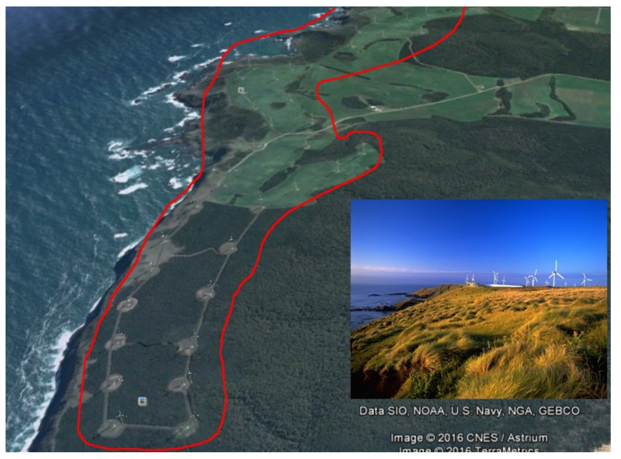
The observational data used in this study is from a wind farm situated along the north-western tip of Tasmania, Australia. The Tasmanian wind farm consists of 37, 1.75 MW wind turbines built in two rows along a 6 km stretch of coastline [22]. Figure 1 (main panel) shows a satellite image of the wind farm (Google Earth). The farm site is circled in red. It features two rows of turbines sitting on a coastal cliff (~100 m above sea level) facing east towards the southern ocean. The northern part of the windfarm is on cleared land, the more southern parts are on native grassland. Sonic anemometers are located 60 m above ground level mounted on the nacelle behind the blades of each of the 37 turbines, taking measurements of wind speed and wind direction. Measurements of wind speed, direction, and power are obtained at 10 min intervals. To obtain better correspondence between the total power output from the wind farm and the measured turbine anemometer wind speeds, an average is taken across all turbines at each of the wind farms.
The NWP used in this study is The Air Pollution Model (TAPM), the model has been run in hind-cast mode for hourly simulations. TAPM is a prognostic meteorological and air pollution model that predicts meteorology parameters and air pollution concentrations. The model was developed by the Commonwealth Scientific and Industrial Research Organisation (CSIRO), and uses the fundamental equations of atmospheric flow, thermodynamics, moisture conservation, turbulence, and dispersion [23]. While the NWP models are computationally more expensive and time consuming, TAPM is user-friendly and fast. However, there are some limitations with this model; it cannot be used for horizontal grid spaces larger than 50 km and it is not suitable for horizontal domain sizes above 1500 km by 1500 km. The use of this model allows quite site specific forecasts, covering a smaller area that can encompass a wind farm site. The simulations were driven using synoptic scale meteorology datasets of NCEP (National Centre for Environmental Prediction) reanalysis data. The temporal resolution of the reanalyses is 3 h and the spatial resolution is 2.5° × 2.5°. TAPM’s domain configuration can be set to have a horizontal resolution in a range of 100 m to 50 km. The model configuration in this study included four successive nested horizontal domains with grid-spacing of 45, 15, 5, 1.5, 0.5 km resolution, respectively. Note that each domain has 25 × 25 grid points and all the grids are centred on the location of the site. Output of the model runs can be at different vertical resolutions, with the level being the height of the model before terrain adjustment. Vertical levels of 10, 25, 50, 75, and 100 m have been investigated. To obtain better correspondence between this forecast data and the measured turbine anemometer observations, another averaging process is performed—averaging of the 10 min observations across all turbines in the wind farm to produce hourly wind farm observations that can be compared to the hourly forecast for the chosen NWP grid point.
Figure 1.
A satellite image of the Woolnorth wind farm sourced from Google Earth (Data SIO NOAA US Navy, NGA, GEBCO, Image CNES/Astrium) [24]. The farm itself is enclosed by the red line. The inset is a photo of the wind farm taken from ground level at the southern end of the wind farm to better indicate the topography and vegetation of the cliff-top location [22].
2.1. Wind Data Analysis
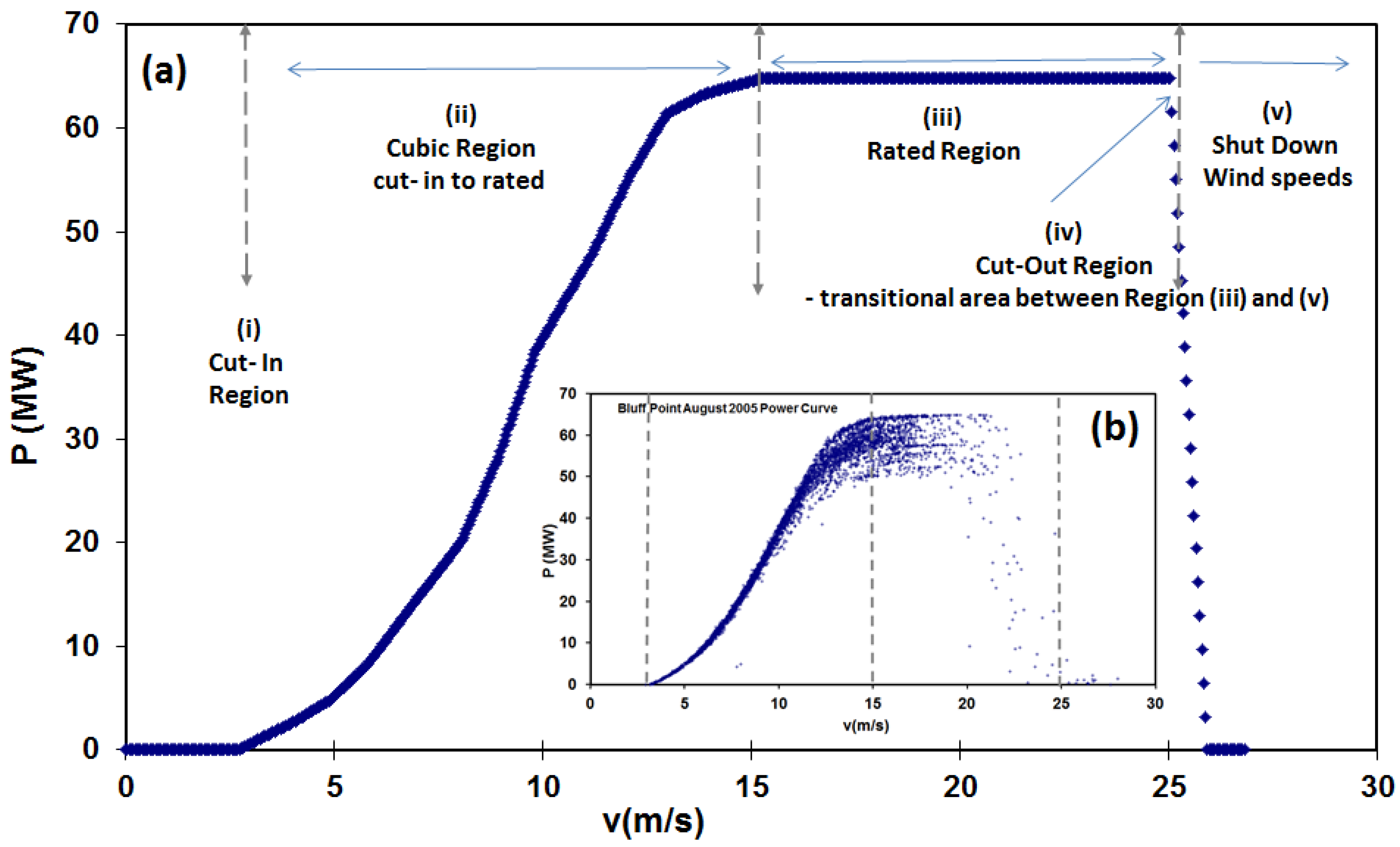
The importance of particular wind speeds and weather events in relation to wind energy forecasting can be explained by the power curve. The power curve shows the expected electrical power output from a wind turbine at different wind speeds. The power in the wind is proportional to the cube of the wind speed. The mass flow rate through the circular area swept by the turbine blades is linear in wind speed v. The resulting power is calculated as the kinetic energy of the air flowing past the turbine per unit time, which is proportional to v2. When combined this gives the cubic dependence above. This relationship ignores effects such as losses due to friction, turbulence, etc. Figure 2a shows the manufacturers power curve for the wind turbines used at the wind farm, scaled to represent the wind farm, and the inset (Figure 2b) shows the power curve for the actual wind farm for August 2005. The main regions of the power curve are identified and labelled in Figure 2a, with the wind speed ranges identified and description of the operational features detailed in Table 1.
Figure 2.
(a) The manufacturers power curve for the turbines on site at Bluff Point. Five regions of interest are identified and labelled (a detailed explanation of each region can be found in Table 1); (b) The actual power curve for Bluff Point for August 2005.
Figure 2.
(a) The manufacturers power curve for the turbines on site at Bluff Point. Five regions of interest are identified and labelled (a detailed explanation of each region can be found in Table 1); (b) The actual power curve for Bluff Point for August 2005.

Table 1.
The different wind speed ranges of the power curve that relate to the regions in Figure 1.
| Region | Wind Speed Range * | Operational Features of Each Region |
|---|---|---|
| ~3 m/s | The wind speed that is sufficient for wind turbine to commence operation |
| ~3–15 m/s | The output power rises approximately as the cube of the wind speed following the wind power equation, Note that the increase in output tapers off as the wind approaches the rated output speed |
| 15–25 m/s | In this region, the power output remains constant despite further increases in wind speed. |
| 25 m/s | This curtailing of output is done deliberately to prevent structural damage to the turbine and typically involves both blade design and active control of blade pitch to “spill” the excess wind energy [25]. |
| >25 m/s | For wind speeds exceeding the cut-off speed, the turbine is shut down to prevent structural/mechanical damage to the turbine. |
Note: * only approximate values based on specific wind turbine.
Sudden changes in wind speed and direction are important for forecasting and operation of wind farms. Figure 2a and Table 1, therefore allows us to identify the main regions of interest for wind energy forecasting, and the most critical considerations are region (ii) and region (iv), which is the boundary between operation at rated output and zero output. These regions are where changes in wind speed have their greatest impact on turbine output. Of these two, region (ii) is arguably the most important, for two reasons. The first reason is the cubic nature of the power curve, where small changes in wind speed can lead to large changes in power output. The second reason is that the measured wind speed sits in this region for most of the time that a turbine is operating. Although wind speeds above the cut-out level are infrequent, they still need consideration due to the sharp change in turbine power output that they cause. Such large and rapid power out transitions can pose particular operational challenges for power system operation. Figure 2b shows the actual power curve for the wind farm. The power is the aggregate power from the full set of turbines on site, plotted against the average wind speed obtained from all of the turbine-mounted anemometers on the wind farm. Our previous work [26] showed that the average of the turbine-mounted anemometers is a more accurate representation of true wind-speed than the meteorological masts at the southern and northern extremities of the site. This work also showed that no significant correction for the influence of the rotor on the turbine-mounted anemometer data was required. The turbine-mounted anemometer data presented here is also uncorrected. Another feature which can be identified from Figure 2b is the large amount of scatter in the wind farm power curve, particularly at higher wind speed ranges. There are two key reasons for this scatter. One is that every wind turbine sees slightly different wind speeds depending on the surrounding terrain, wind direction, atmospheric conditions and, in some cases, wake effects from other turbines. Using only one or two anemometers to measure the wind speed for a wind farm cannot precisely capture the actual wind speeds seen by each of the turbines under different conditions. Another reason is that wind turbines are controlled to face into the direction of the wind, however, the turbine will not always turn (yaw) for small changes in wind direction, a threshold yaw error of between 8 and 15 degrees averaged over a duty cycle depending on the control strategy used by the wind turbine. Because of this, we can lose a significant portion of the wind energy when the wind blows from a slightly different direction as only the perpendicular component of the wind to the turbine rotor will provide power, which is illustrated by the scatter in the power curve in Figure 2b.
3. Correction Methodology and Forecast Verification
There are different measures of forecast error that allow us to focus on one or many aspects of forecast quality [27,28]. Bias is detected statistically as a difference between the means of the historical forecast and historical observation distributions. In terms of forecasting, this establishes whether a forecast systematically over- or under-predicts against observations. Bias is one of the key errors found in NWP forecasts as identified by Woodcock and Engel [29]. Previous work [30] has investigated a bias correction methodology based on the trimean or Best Easy Systematic (BES) estimator:
where the quartiles Q1, Q2, and Q3 statistically divide the distribution over the forecast errors in the sample size into the lowest 25% of the data, the median, and the highest 25%, respectively [31,32]. The forecast error is calculated as the observation minus the forecast. Equation (1) is essentially a weighted average of the quartiles with a heavier weighting given to the median. This statistical approach contains enough information within the distribution about the extreme values yet, at the same time, does not have them disproportionally contribute to the applied correction.
For correcting the wind speed, a statistical measure needs to be robust and sensitive to extreme values as wind speed can vary quite rapidly across a wind farm site. An analysis of past forecasts and observations can accurately determine the bias in a forecast as it is a systematic error. This can then be corrected for in the process of producing new forecasts. There are a number of factors to consider in developing a bias correction methodology. The BES is calculated from the previous hours forecast error, i.e., if the BES is calculated at time t, the BES bias window will calculate the quartiles from t − 1 to t − n, where n is the bias window length.
Initial investigations were carried out using simple linear and multiple regression, however, neither of these measures were able to cope with extreme wind speed events or sudden changes in wind speed.
Before a corrected prediction can be calculated, conditions are put in place that identify the sign of the forecast error and the sign of the BES to ensure that the new forecast is correctly adjusted. A bias Corrected Prediction (CP) is produced by adding or subtracting the BES from the future hour’s NWP prediction.
The CP methodology described above, enhances the forecast accuracy. When applied to the TAPM forecasts. For this wind farm site, improvements of approximately 10% were achieved. The full details are discussed in Section 4. However, further improvement can be obtained by applying an additional correction to account for position and timing factors. A primary concern in wind forecasting is predicting sudden changes in wind speed and direction, and the timing and resolution of NWP models do not adequately capture those specific events [3]. Although the resulting Corrected Prediction (CP) is an improvement on an uncorrected forecast the above mentioned factors are not taken into account in the simple bias correction methodology. Therefore, after applying the CP methodology, an extra correction (referred to in the text below as a Double Corrected Prediction—DCP) is applied to improve not just the accuracy, but also some of the timing and scale errors, associated with the forecast.
The DCP is implemented by a smoothing weighted average, taking the weighted sum of the corrected prediction and an observation Ot−10 made some time t earlier:
where the smoothing factor 0 < α < 1. Because the observations are obtained at 10 min intervals Ot−10 is taken as the observation at 10 min to the hour at which CP is made. For the work I used α = 0.5, which was found to provide the best results for both cases where the forecast errors are large and small.
A comparison was also made with the forecast methods against persistence and an exponential smoothing of past observations, with the DCP method outperforming both.
Forecast verification is crucial in determining the performance of any model. The most common verification methods are the Root Mean Square Error (RMSE) and Mean Bias Error (MBE). The RMSE puts a larger weighting on large errors, which for sudden changes in wind speed and extreme events, can be a useful indicator of model performance.
4. Results
4.1. Assessment of TAPM for Wind Forecasting
The mesoscale NWP model used in this study was TAPM. TAPM has an advantage in that it does not require a large amount of computational time compared to other NWP models, and it allows quite point specific forecasts, which when covering a wind farm area, can be incredibly useful. This is especially the case when the resolution of the model can vary from 500 m to 45 km. The first series of simulations was to identify which horizontal resolution was the optimum for running the model. The model centre was chosen as the central point of the wind farm. As discussed in Section 2, TAPM was run for all of 2005 at horizontal resolutions of 45 km, 15 km, 5 km, 1.5 km, and 500 m. Figure 3 shows the % RMSE normalized with respect to the average observations from the wind farm. Overall, forecasts appear better during the winter months (JJA), with larger errors experienced in the warmer months (NDJ). The southern part of Australia can experience highly variable weather in summer, hence the model is not as good at capturing these changes. The optimum resolution overall was that of 5 km. The model also had the best performance in the winter months, particularly August. This fact is quite interesting as an extreme weather event occurred in late August. Sudden changes in wind speed or direction can change the output of a wind farm from full power to zero output in a matter of minutes—these extreme wind events are therefore of particular importance to developing useful forecasts for the electricity industry.
Figure 3.
The % normalized RMSE with respect to the average for TAPM horizontal resolutions of 45 km, 15 km, 5 km, 1.5 km, and 500 m for each month of 2005.
Figure 3.
The % normalized RMSE with respect to the average for TAPM horizontal resolutions of 45 km, 15 km, 5 km, 1.5 km, and 500 m for each month of 2005.
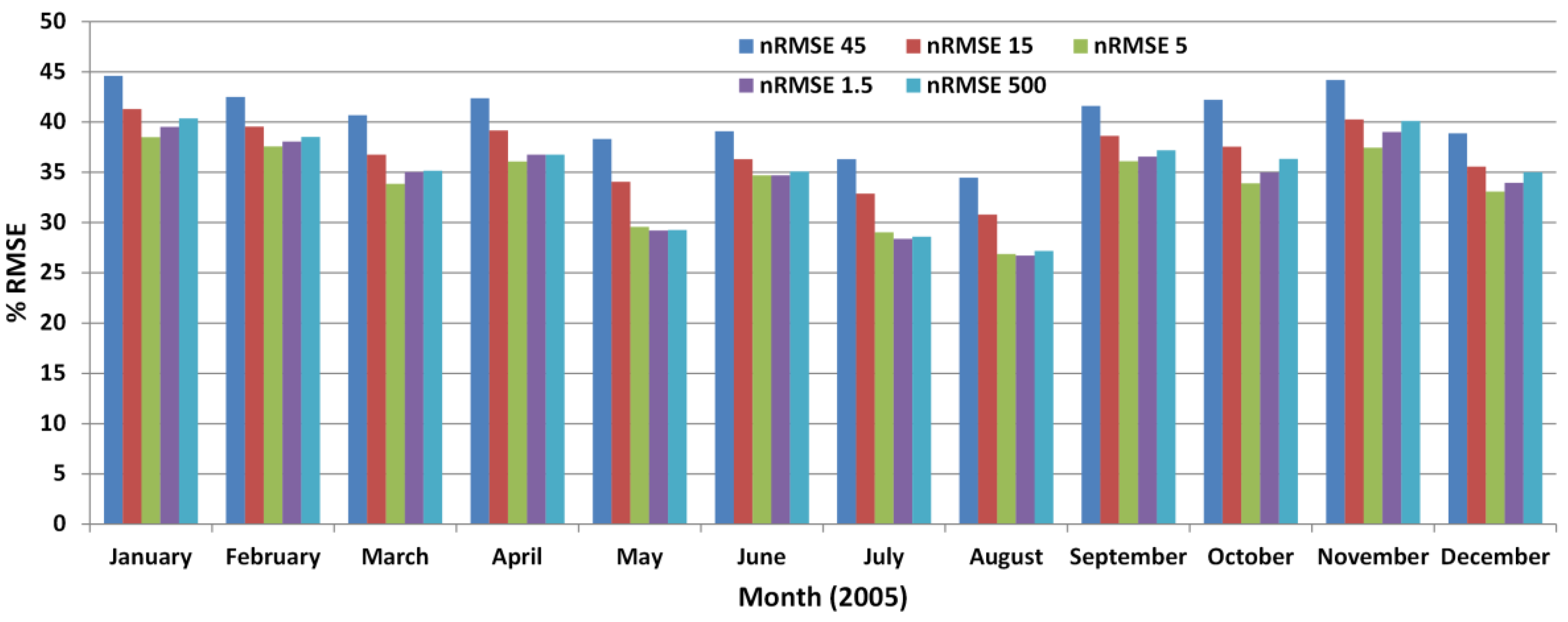
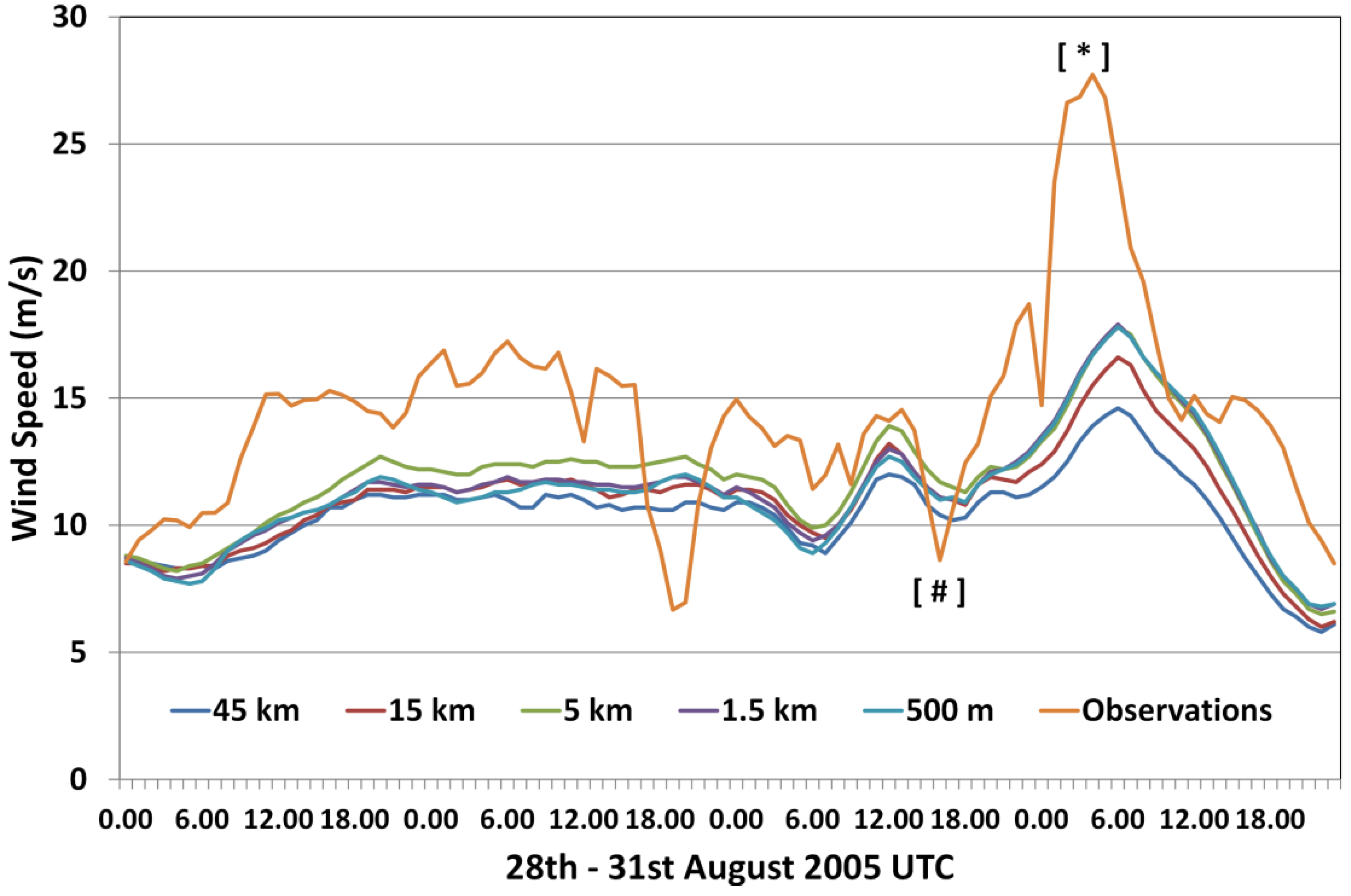
Figure 4 illustrates the days leading up to the extreme event (28th–31st August 2005) that lasted for a period of approximately four hours spanning the 30–31 August 2005. There are two main important features illustrated in Figure 4, the sudden drop in wind speed occurring on the 30 August, highlighted by #, and the sudden and prolonged increase in wind speed over 25 m/s occurring around 00:00 UTC on the 31 August highlighted by *. The meteorological features identified as the cause of this extreme wind event were a deepening low pressure system, accompanied by a strong front and trough following closely behind [26]. This in turn kept wind speeds high for a prolonged period. Figure 4 shows both observational data from the wind farm and all the TAPM horizontal simulations. It is immediately clear that the 5 km resolution performs the best, however during the extreme event there is minimal difference between the 500 m, 1.5 km, and 5 km resolutions. This seems to indicate that the finer the resolution, the better the performance during extreme events. For all resolutions there are noticeable magnitude errors, and the intra hour variability is not captured as well with TAPM.
Figure 4.
TAPM forecasts at all resolutions and the wind farm observations over the period 28th–31st August 2005.
Figure 4.
TAPM forecasts at all resolutions and the wind farm observations over the period 28th–31st August 2005.
Another avenue of investigation is to see whether utilizing the surrounding grid points of TAPM can produce a more accurate forecast. If we consider that the wind farm spans approximately 5 km along the coast, with 2 rows of turbines spaced within a distance of approximately 2 km, we can utilise the forecast at each grid point to represent a grouping of wind turbines, and use the average of those forecasts to compare to the wind farm average we have previously calculated. Figure 5 shows the horizontal layout within TAPM, with the black box representing the forecast grid area, which encompasses 24 individual forecasts at a horizontal resolution of 500 m between each grid point.
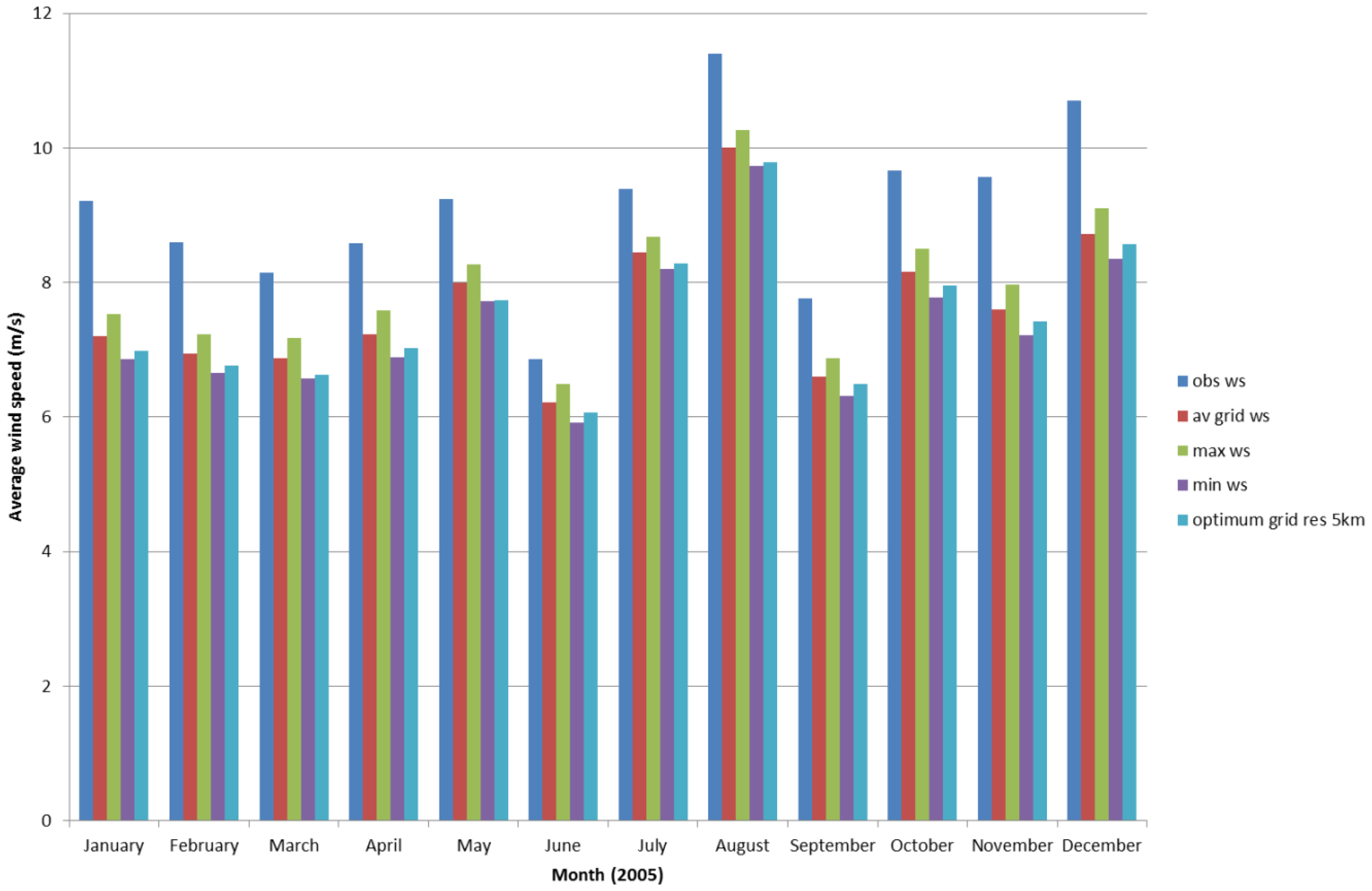
Figure 6 shows the observed wind farm average, the average of all surrounding grid points, the maximum forecast, minimum forecast, and optimum forecast. Overall, the average of all grid points is closer than the 5 km resolution, with an improvement in RMSE by approximately 1% each month, but what is interesting is that the maximum forecast wind speed is the closest to the observed wind farm data for all months, another indication that TAPM mostly under-predicts the wind speed. The maximum wind speed did not always come from the same one grid point, and at times many grid points reported the same value, therefore for the remainder of this study I will use the optimum and average of the grid points.
Figure 5.
TAPM forecast grids, with the central point the centre of the wind farm. The black box shows the area encompassing the surrounding grid points.
Figure 5.
TAPM forecast grids, with the central point the centre of the wind farm. The black box shows the area encompassing the surrounding grid points.
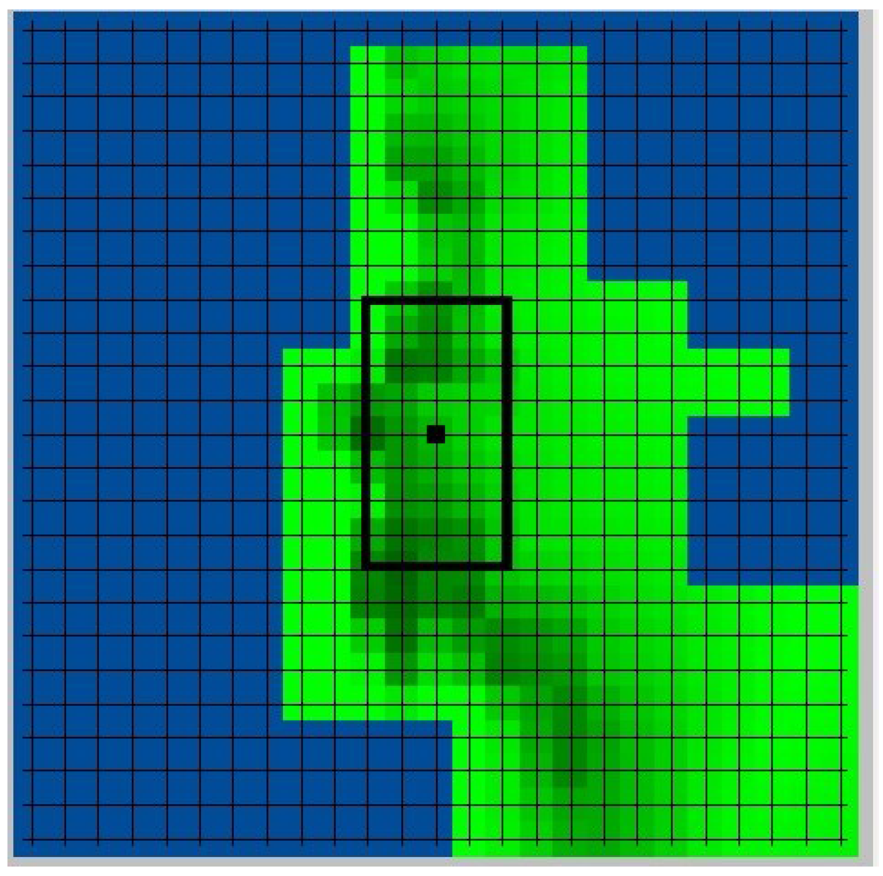
Figure 6.
Average wind speed observations for each month of 2005 for the observations, the average of all the grid surrounding grid points, the maximum and minimum wind speed from the surrounding grid points, and the optimum resolution of 5 km found earlier.
Figure 6.
Average wind speed observations for each month of 2005 for the observations, the average of all the grid surrounding grid points, the maximum and minimum wind speed from the surrounding grid points, and the optimum resolution of 5 km found earlier.

4.2. Correction Methodology Analysis
The results presented in this section will cover everyday operation of the wind farm, as well as an extreme weather event, all which occurred within a week’s operation (25–31 August 2005) of the wind farm. For all corrections methodologies, the CP and DCP results were obtained using a 48 h bias window. A bias window of 48 h was chosen, after investigating the effect of bias window width by considering four different window lengths (24 h, 48 h, 7 days, and 14 days). There was a minimal difference between a 24 h and 48 h bias window, but overall the 48 h bias window had the lowest RMSE and MAE. Increasing the bias window beyond 48 h resulted in a minimal decrease to the resulting forecast accuracy, and as a result, I completed the remainder of the study with a 48 h bias window.
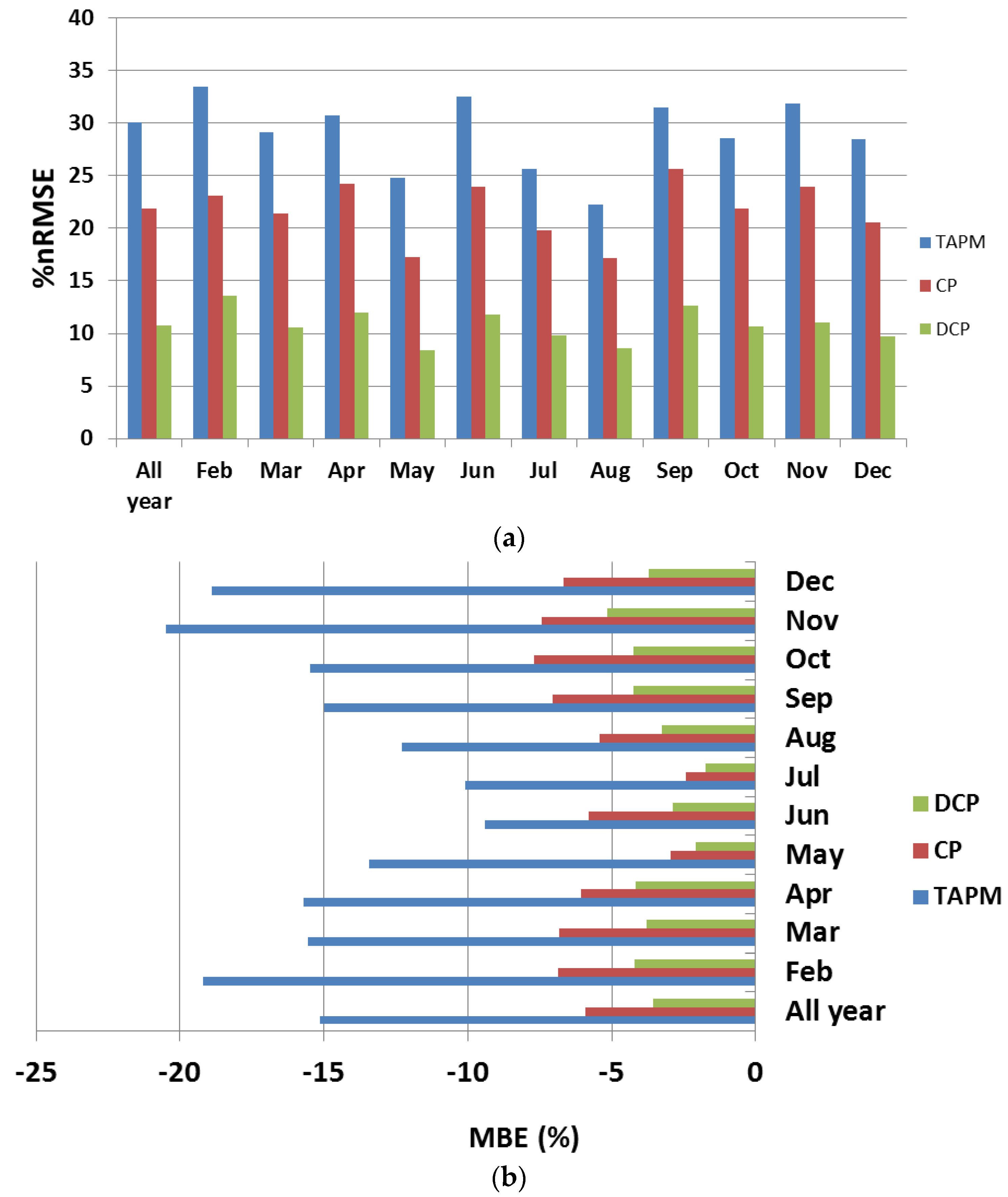
The results from a study of the performance of the CP and DCP forecasts for everyday operation of the wind farm is presented first. Figure 7a shows the % normalised RMSE with respect to the average observations for TAPM, CP, and DCP for each month of 2005, as well as the whole year. Observational data for January was sparse, so it was removed from the analysis. For each month, the RMSE CP error is reduced by up to 10%, however, the most notable aspect is that the DCP error is generally ~50% smaller than the other two methods throughout the whole year. Figure 7b shows the MBE for the same period as Figure 7a. It is clear that TAPM severely under-predicts, however this is reduced to under 5% across all seasons with the implementation of the DCP. This improvement holds potential significance for wind farm management and the scheduling of controllable (dispatchable) generation within the power system to meet future demand. Improving wind speed forecasts will facilitate the successful integration of wind generation within the electricity industry.
Figure 7.
(a) The % nRMSE with respect to the average observations for TAPM, CP, and DCP for each month and all year, (b) As for (a) but with respect to MBE.
Figure 7.
(a) The % nRMSE with respect to the average observations for TAPM, CP, and DCP for each month and all year, (b) As for (a) but with respect to MBE.
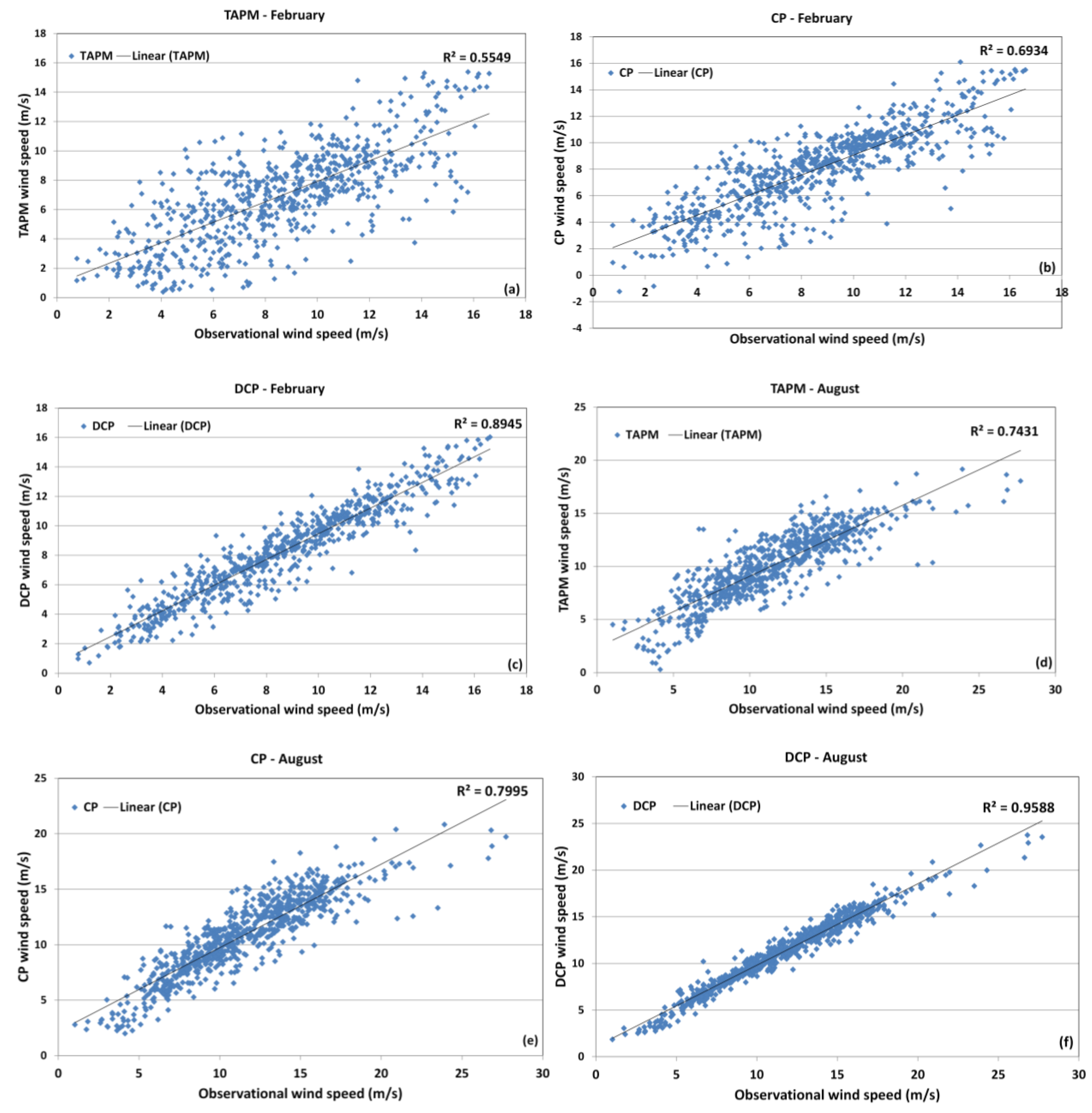
To investigate the spread in the data for specific months, I now drill down into specific time periods, two months within the two extreme seasons, Winter—August and Summer—February, to demonstrate that the enhanced effectiveness of DCP holds more specifically. Figure 8a–c show a scatter plot of TAPM, CP, and DCP, respectively for February and Figure 8d–f for August. Even though from Figure 7, August had one of the best RMSE and MBE, it does contain an extreme wind event, which will be discussed further in the next section.
Figure 8.
(a–c) Scatter plot of TAPM forecasts, CP forecasts and DCP forecasts against the wind farm observations for February 2005; (d–f) As for (a–c) but August 2005.
Figure 8.
(a–c) Scatter plot of TAPM forecasts, CP forecasts and DCP forecasts against the wind farm observations for February 2005; (d–f) As for (a–c) but August 2005.

Each of the months in Figure 8 shows that forecasts improved with each correction methodology, most noticeable in August. February, however can fall into an unpredictable season, with greater variability in weather and lower than average wind speeds, with TAPM experiencing higher errors in the lower wind speed ranges. The real improvement can also been seen from the R2 values in each graph, ranging from 0.56–0.89 in February and 0.74 to 0.96 in August.
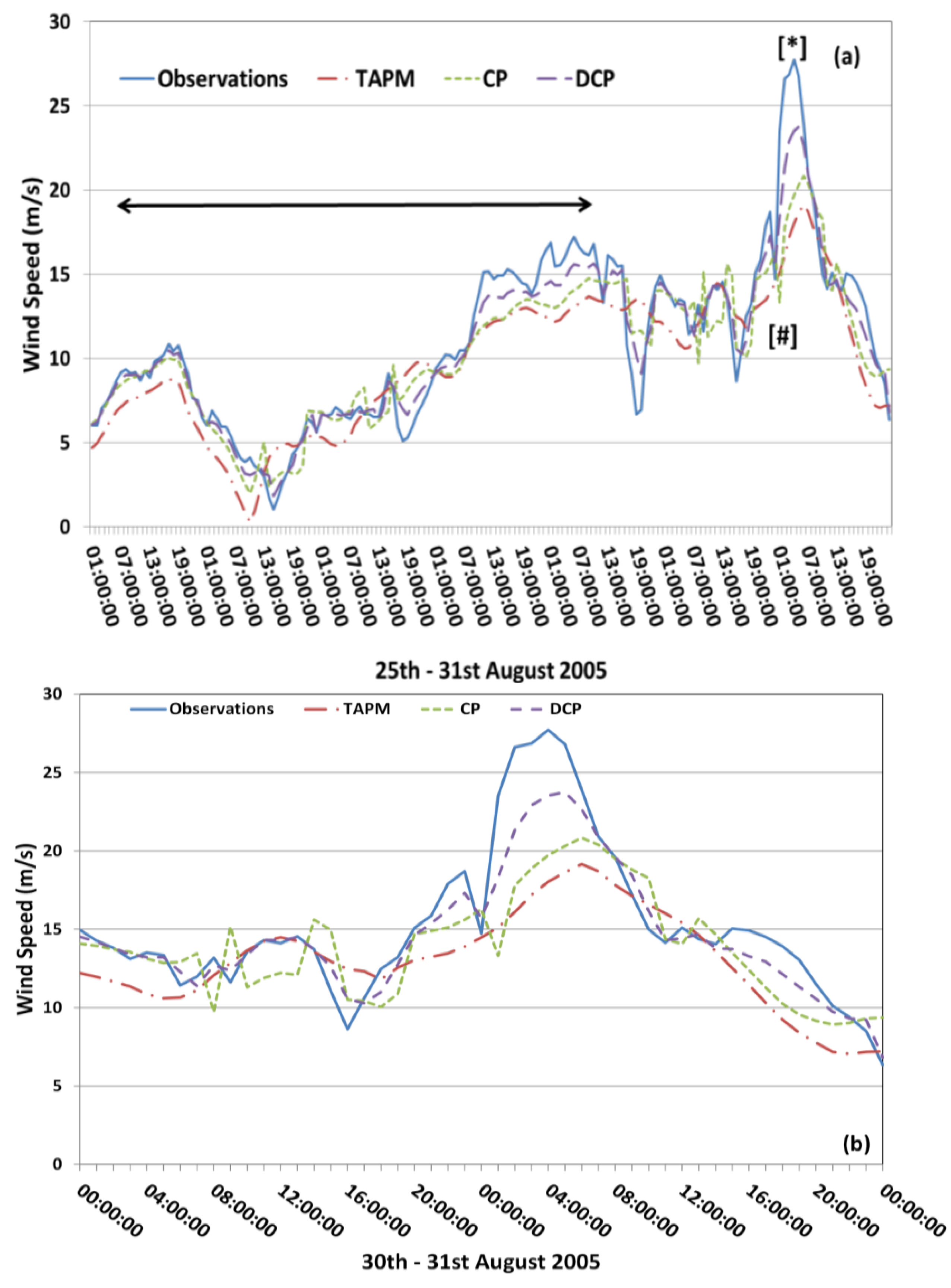
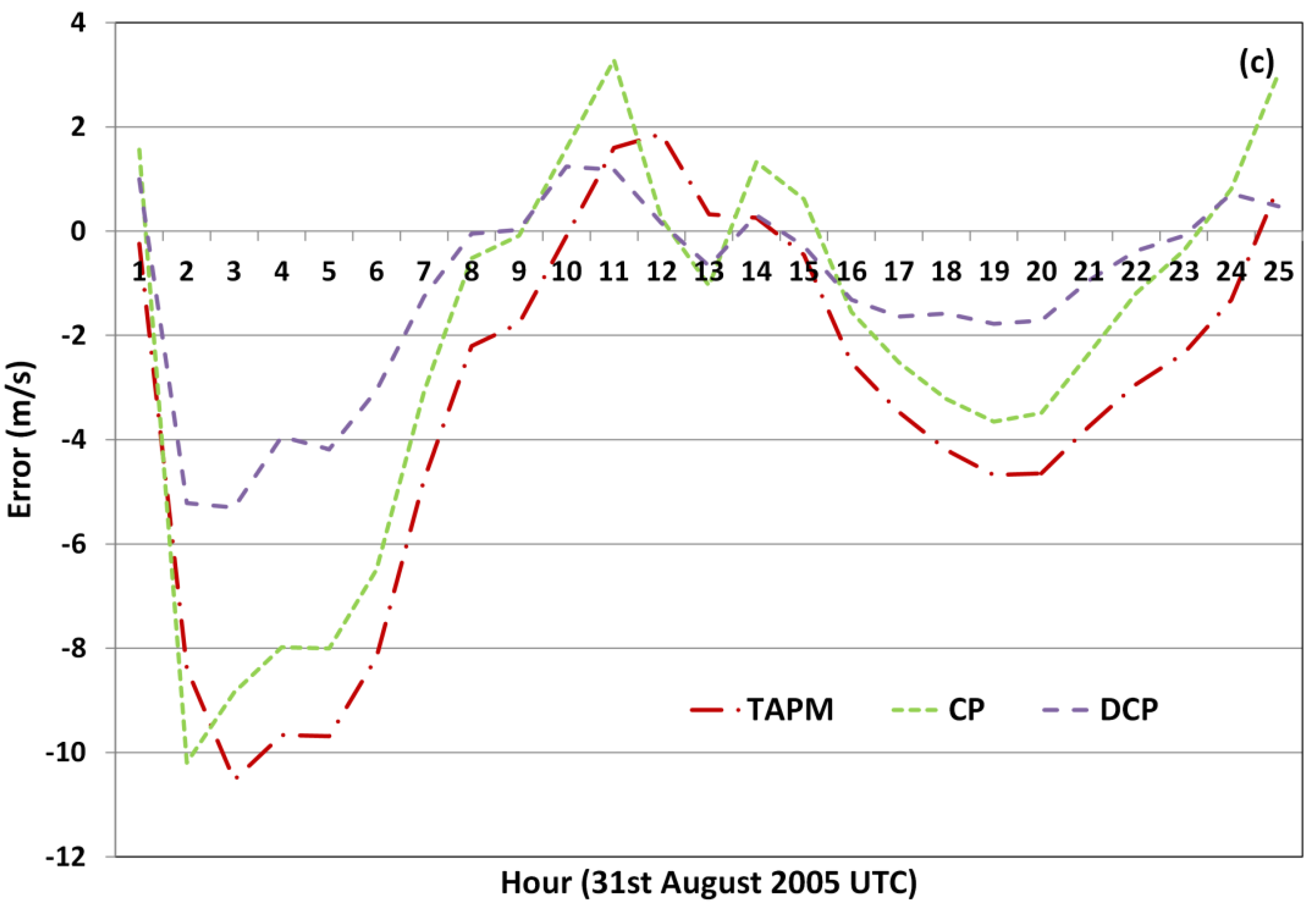
The improvement in wind speed forecast accuracy overall led to the next investigation of forecast performance—how well do the correction methodologies improve the forecasting of extreme wind events? Sudden changes in wind speed or direction can change the output of a wind farm from full power to zero output in a matter of minutes—these extreme wind events are therefore of particular importance to developing useful forecasts for the electricity industry. Figure 9a shows the week covering the 25th–31st August 2005, which encompasses everyday operation of the wind farm, as well as an extreme weather event for TAPM, CP, and DCP models. The region highlighted with ↔ covers day to day operation of the wind farm. Overall the DCP has been better able to capture the timing as well as magnitude changes, compared to the CP, where timing issues still were a problem. A sudden drop in wind speed occurring on the 30 August is highlighted by #, and the sudden and prolonged increase in wind speed over 25 m/s occurring around 00:00 UTC on the 31 August highlighted by *. Figure 9b is an enlargement of the extreme wind event. The region highlighted by # shows that TAPM and the CP incorrectly predicted the magnitude and direction of the short timescale dip in wind speed. The DCP is an improvement over the uncorrected prediction and CP, but this method was still not able to fully show that there would be a sudden dip in the wind speed. This figure highlights the apparent inability of TAPM to predict this wind speed event, for both timing and magnitude. TAPM under-predicted the wind speed for a majority of the time over the 48 h period. It is clear that the DCP is an improvement over the uncorrected prediction for both the magnitude and timing of the wind speed event, as illustrated by the region denoted *. To quantify the error, Figure 9c shows the magnitude error in wind speed for the bias corrected forecasts, CP and DCP along with the original uncorrected TAPM predictions for the 24 h period. There is a clear skew towards under-prediction of wind speed. The CP forecast has improved some of the magnitude issues over most of the 24 h period, but timing issues are still a problem. Some of this is related to the fact that any correction to the forecast is based on the forecast error the previous hour, hence there are times where the CP actually becomes the poorer performer. However, the most noticeable improvement in accuracy is in the DCP. For this extreme wind event the DCP has successfully reduced the forecast error by at least 50%.
Figure 9.
(a) Observations for the wind farm, TAPM predictions, and the CP and DCP forecasts with a 48 h bias window covering the period 25th–31st August 2005, illustrating various wind speed regimes experienced by the wind farm over a week—general day to day operation, highlighted by ↔ and an extreme wind event that occurs over the 31st August 2005. The main features of the extreme event are highlighted by #, and *; (b) zooming down into the extreme event in Figure 9a; (c) the magnitude error for each of the forecasts for the 24 h period covering the extreme event on the 31st August 2005.


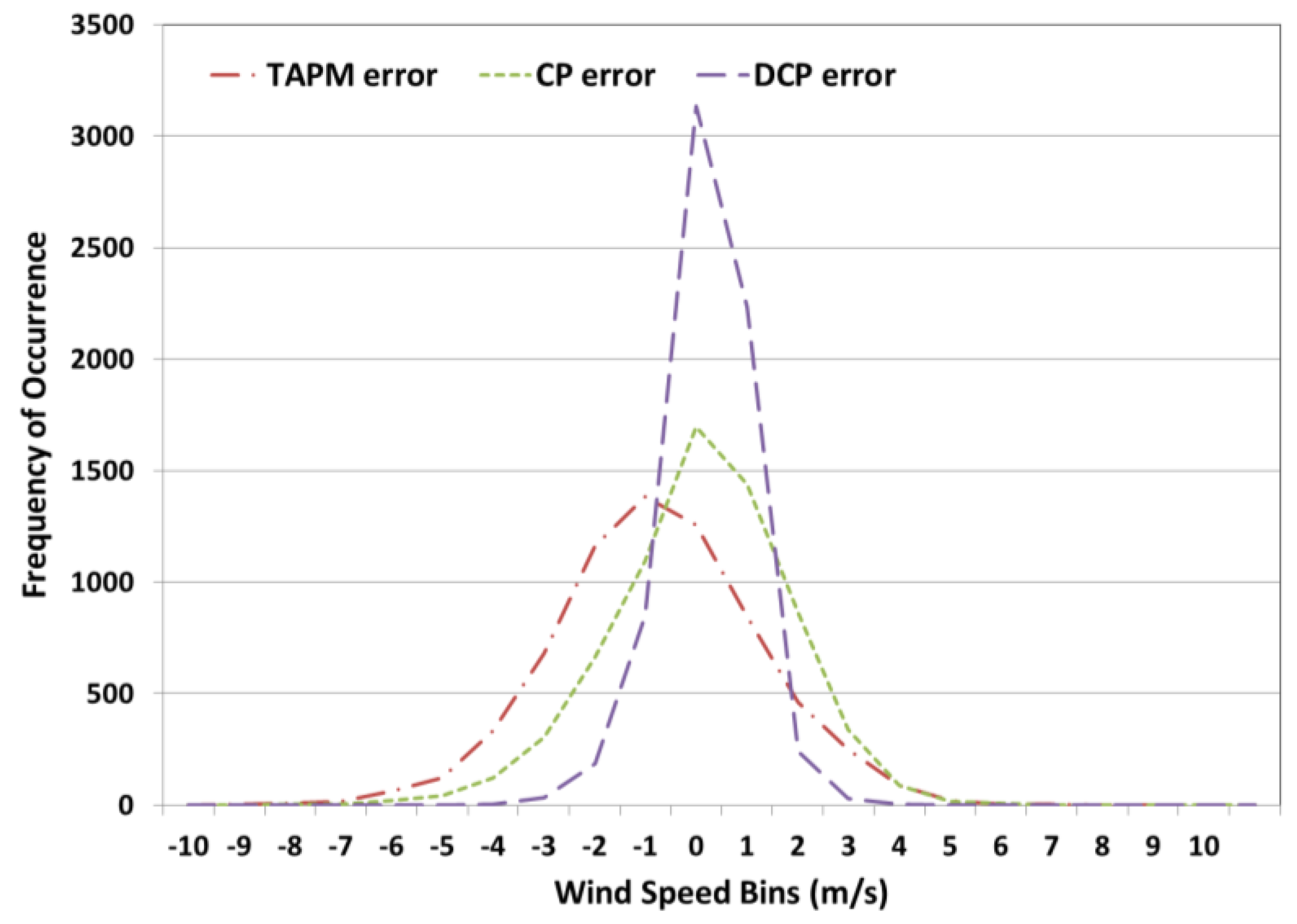
The next test of performance for the correction methodologies is again related back to the cubic relationship between wind speed and power introduced in Section 2.1, and is to investigate how often the various forecasts over or under predicted an observation within the region 3–15 m/s, which is where errors of more than 3 m/s can affect a power forecast. If your wind speed is doubled, it reflects in an increase in power by a factor of 8, if we relate the values back to the wind power equation. Figure 10 shows a histogram of the frequency of occurrence of wind speed errors for TAPM, CP, and DCP from January 2005–December 2005 for wind speed ranges within 3–15 m/s. The shape and peak of the histogram narrows with the implementation of the CP and DCP. The figure also shows a clear skew towards under prediction for all wind speed ranges. Implementation of the bias correction methodologies also lead to a decrease in the tail of the distribution which indicates that larger errors have been reduced.
The DCP method however has successfully brought down the percentage of occurrences of under and over prediction for the year.
Figure 10.
A histogram of the frequency of occurrence of wind speed errors for the TAPM predictions, the CP methodology and the DCP methodology for wind speeds within 3–15 m/s over 2005.
Figure 10.
A histogram of the frequency of occurrence of wind speed errors for the TAPM predictions, the CP methodology and the DCP methodology for wind speeds within 3–15 m/s over 2005.
5. Conclusions
Intermittent renewable generation is achieving higher levels of penetration within power systems globally. It is therefore becoming increasingly important to provide useful forecasts for this generation to manage ongoing supply demand balance in the electricity industry. Weather forecasting within the power sector to date has largely concentrated on how the weather, particularly temperature, affects consumers’ power usage and hence overall system demand. However, supply side forecasting is becoming an increasingly important component in managing the power system. This study investigated the potential to improve the accuracy and timing of wind speed forecasts by the application of a correction methodology for wind energy forecasting. The Bluff Point wind farm chosen for the case study often experiences highly variable and extreme wind events due to its location along a steep cliff, and also lying in the path of the roaring forties—a region notable for strong winds. Results concentrated on wind speed ranges which if incorrectly forecast could cause the greatest discrepancy to wind power output and power management and covered the period January 2005–December 2005. For the Bluff Point wind farm, there was a systematic under-prediction for a majority of wind speed events.
The optimum bias window was found to be 48 h after numerous bias windows were tested. The bias methodologies improved the prediction for the wind speed events that were investigated, with the wind speed error more than halved by the DCP methodology for general wind speed conditions as well as an extreme wind event. An improvement in the errors was evident in both magnitude and timing of wind speed events.
For the more extensive time series, the frequency of under prediction was reduced by approximately 13% across the whole year by the DCP method in the wind speed rang 3–15 m/s. The use of the bias correction methodology has been shown to greatly enhance the timing and accuracy of forecasts from the NWP, with the use of actual wind farm data providing an added benefit to the forecast to better represent the wind farm. It has also provided improvement in forecast accuracy for model spin-up issues.
Acknowledgments
The author wish to thank Hydro Tasmania and Roaring 40s for access to the Woolnorth wind farm data.
Conflicts of Interest
The author declare no conflict of interest.
References
- Feinberg, E.A.; Genethliou, D. Load Forecasting. In Applied Mathematics for Restructured Electric Power Systems: Optimization, Control, and Computational Intelligence; Chow, J.H., Wu, F.F., Momoh, J.J., Eds.; Spinger: New York, NY, USA, 2005; pp. 269–285. [Google Scholar]
- Sanchez, I. Short-term prediction of wind energy production. Int. J. Forecast. 2006, 22, 43–65. [Google Scholar] [CrossRef]
- Archer, C.L.; Jacobson, M.Z. Evaluation of global wind power. J. Geophys. Res. 2005, 11, D1211. [Google Scholar] [CrossRef]
- Wiser, R.; Bolinger, M. 2011 Wind Energy Technologies Market Report; Lawrence Berkeley Laboratories, US Department of Energy: Oak Ridge, TN, USA, August 2012. [Google Scholar]
- Möhrlen, C.; Jørgensen, J.U. A new algorithm for Upscaling and Short-term forecasting of windpower using Ensemble forecasts. In Proceedings of the 8th International Workshop on Large-Scale Integration of Wind Power into Power Systems as well as on Transmission Networks for Offshore Wind Farms, Bremen, Germany, 14–15 October 2009.
- Wind Energy Forecasting, a Collaboration of the National Centre for Atmospheric Research (NCAR) and Xcel Energy. Available online: http://www.nrel.gov/docs/fy12osti/52233.pdf (accessed on 10 July 2015).
- Blonbou, R. Very Short Term Wind Power Forecasting with Neural Networks and Adaptive Bayesian learning. Renew. Energy 2011, 36, 1118–1124. [Google Scholar] [CrossRef]
- Marquis, M.; Wilczak, J.; Ahlstrom, M.; Sharp, J.; Stern, A.; Smith, J.C.; Calvert, S. Forecasting the Wind to Reach Significant Penetration Levels of Wind Energy. Bull. Am. Meteorol. Soc. 2011, 92, 1159–1171. [Google Scholar] [CrossRef]
- Foley, A.M.; Leahy, P.G.; Marvuglia, A.; McKeogh, E.J. Current methods and advances in forecasting of wind power generation. Renew. Energy 2012, 37, 1–8. [Google Scholar] [CrossRef] [Green Version]
- Junk, C.; Monache, L.D.; Alessandrini, S.; Cervone, G.; von Bremen, L. Predictor-weighting strategies for probabilistic wind power forecasting with an analog ensemble. Meteorol. Z. 2015, 24, 361–379. [Google Scholar]
- Milligan, M.; Schwartz, M.; Wan, Y. Statistical Wind Power Forecasting Models: Results for U.S. Wind Farms; National Renewable Energy Laboratory: Golden, CO, USA, 2003; p. 17.
- Torres, J.L.; Garcia, A.; de Blas, M.; Francisco, A. Forecast of hourly averages wind speed with ARMA models in Navarre. Sol. Energy 2005, 70, 65–77. [Google Scholar] [CrossRef]
- Potter, C.W.; Negnevitsky, M. Very short-term wind forecasting for Tasmanian power generation. IEEE Trans. Power Syst. 2006, 21, 965–972. [Google Scholar] [CrossRef]
- Agrawal, M.; Boland, J.; Ridley, B. Analysis of wind farm output: Estimation of volatility using high frequency data. Environ. Model. Assess. 2013. [Google Scholar] [CrossRef]
- Vincent, C.; Bourke, W.; Kepert, J.D.; Chattopadhyay, M.; Ma, Y.; Steinle, P.J.; Tingwell, C.I.W. Verification of a high-resolution mesoscale NWP system. Aust. Meteorol. Mag. 2008, 57, 213–233. [Google Scholar]
- Huang, X.; Ma, Y.; Mills, G. Verification of Mesoscale NWP Forecasts of Abrupt Wind Changes; CAWCR Technical Report No. 008; The Centre for Australian Weather and Climate Research: Melbourne, Australia, 2008; p. 72. [Google Scholar]
- Giebel, G.; Landberg, L.; Kariniotakis, G.; Brownsword, R. State-of-the-Art on Methods and Software Tools for Short-Term Prediction of Wind Energy Production; EWEC: Madrid, Spain, 2003. [Google Scholar]
- Landberg, L.; Giebel, G.; Nielsen, H.A.; Nielsen, T.; Madsen, H. Short-term prediction—An overview. Wind Energy 2003, 6, 273–280. [Google Scholar] [CrossRef]
- Focken, U.; Lange, M. Final report—Wind power forecasting pilot project in Alberta, Canada. In Wind Power Forecasting PILOT Project; Energy & Meteo Systems: Oldenburg, Germany, 2008; p. 21. [Google Scholar]
- Jørgensen, J.; Möhrlen, C. AESO wind power forecasting PILOT project: Final project report. In Wind Power Forecasting PILOT Project; Weprog: Ebberup, Denmark, 2008; p. 102. [Google Scholar]
- Shi, J.; Guo, J.M.; Zheng, S.T. Evaluation of Hybrid Forecasting Approaches for Wind Speed and Power Generation Time Series. Renew. Sustain. Energy Rev. 2012, 16, 3471–3480. [Google Scholar] [CrossRef]
- Roaring 40s. Available online: http://www.hydro.com.au/energy/our-power-stations/wind-power (accessed on 18 November 2015).
- Hurley, P. TAPM V4. Part 1: Technical Description; CSIRO Marine and Atmospheric Research Paper No. 25; Commonwealth Scientific and Industrial Research Organisation: Canberra, Australia, 2008. [Google Scholar]
- Google Earth (Data SIO NOAA US Navy, NGA, GEBCO, Image CNES/Astrium). Available online: https://www.google.com/maps/@-40.729434,144.6883667,9879m/data=!3m1!1e3 (accessed on 18 January 2016).
- Manwell, J.F.; McGowan, J.G.; Rogers, A.L. Wind Energy Explained, Theory, Design and Application; John Wiley & Sons Ltd.: West Sussex, UK, 2006. [Google Scholar]
- Kay, M.J.; Cutler, N.; Micolich, A.; MacGill, I.; Outhred, H. Emerging Challenges in Wind Energy Forecasting for Australia. Aust. Meteorol. Ocean. J. 2009, 58, 99–106. [Google Scholar]
- Murphy, A.H. What is a good forecast? An essay on the nature of goodness in weather forecasting. Weather Forecast. 1993, 8, 281–293. [Google Scholar] [CrossRef]
- Murphy, A.H. The coefficients of correlation and determination as measures of performance in forecast verification. Weather Forecast. 1995, 10, 681–688. [Google Scholar] [CrossRef]
- Woodcock, F.; Engel, C. Operational Consensus Forecasts. Weather Forecast. 2005, 20, 101–111. [Google Scholar] [CrossRef]
- Kay, M.; MacGill, I. Improving NWP Forecasts for the Wind Energy Sector. In Weather Matters for Energy; Springer: New York, NY, USA, 2014. [Google Scholar]
- Wonnacott, T.H.; Wonnacott, R.J. Introductory Statistics; Wiley: New York, NY, USA, 1977; p. 650. [Google Scholar]
- Tukey, J.W. Exploratory Data Analysis; Addison-Wesley: Reading, MA, USA, 1977; p. 688. [Google Scholar]
© 2016 by the author; licensee MDPI, Basel, Switzerland. This article is an open access article distributed under the terms and conditions of the Creative Commons by Attribution (CC-BY) license (http://creativecommons.org/licenses/by/4.0/).
Share and Cite
MDPI and ACS Style
Kay, M. The Application of TAPM for Site Specific Wind Energy Forecasting. Atmosphere 2016, 7, 23. https://doi.org/10.3390/atmos7020023
AMA Style
Kay M. The Application of TAPM for Site Specific Wind Energy Forecasting. Atmosphere. 2016; 7(2):23. https://doi.org/10.3390/atmos7020023
Chicago/Turabian StyleKay, Merlinde. 2016. "The Application of TAPM for Site Specific Wind Energy Forecasting" Atmosphere 7, no. 2: 23. https://doi.org/10.3390/atmos7020023
Note that from the first issue of 2016, this journal uses article numbers instead of page numbers. See further details here.