Rain Attenuation Correction of Reflectivity for X-Band Dual-Polarization Radar

Abstract

In order to improve the performance of X-band dual-polarization radars, it is necessary to conduct attenuation correction before using the X-band radar data. This study analyzes a variety of attenuation correction methods for the X-band radar reflectivity, and proposes a high-resolution slide self-consistency correction (SSCC) method, which is an improvement of Kim et al.’s method based on Bringi et al.’s original method. The new method is comprehensively evaluated with the observational data of convective cloud, stratiform cloud, and the stratiform cloud with embedded convection. Comparing with the intrinsic reflectivity at X-band calculated from the reflectivity at S-band, it is found that the new method can effectively reduce the correction errors when calculating differential propagation shift increments using the conventional self-consistency attenuation correction method. This method can efficiently correct the X-band dual-polarization radar reflectivity, in particular, for the echoes with reflectivity greater than 35 dBZ.

1. Introduction

Comparing with the conventional Doppler weather radar, dual-polarization radars can measure more valuable polarized information precipitation systems. The polarized information allows to improve the accuracy of radar-based quantitative precipitation estimation, raindrop size distribution (DSD) retrieval and precipitation particle identification [1,2,3,4,5,6,7,8,9,10]. Previous studies on the application of dual-polarization radars are mostly designed for S, C-band radars [11,12,13,14,15]. Research on X-band dual-polarization radars is limited, since X-band radars experience severe attenuation compared to S, C-band radars. However, due to their low cost, small antennas, easy mobility and high temporal and spatial resolution, X-band dual-polarization radars have become an important detection equipment in the areas of cloud and precipitation physics and weather modification. In order to improve the performance of X-band dual-polarization radars, the attenuation needs to be corrected before application.

Atlas and Banks [16] showed there were two main factors resulting in attenuation. One is detection range, whereby the echo power received by the radar will decrease with increasing range, and this applies to all radar wavelengths; the other is rain attenuation. With the exception of intense storms, rain attenuation for electromagnetic waves with a wavelength greater than approximately 7 cm is negligible. Zhang et al. [17] noted that the first attenuation factor is mainly because gas molecules absorb electromagnetic waves and the influence of scattering can be neglected. The absorption attenuation of electromagnetic waves with a wavelength greater than 2 cm is generally small, but when the wavelength is approximately 1 cm or the detection range is large, the attenuation caused by the first factor still needs to be considered. Therefore, the attenuation at X-band (about 3 cm in wavelength) is mainly due to the second factor.

The conventional method of attenuation correction for single-polarization radars is mostly based on the empirical relationship between horizontal reflectivity factor Z_H and rainfall intensity R(Z_H = aR^b; a, b are empirical constants). This method retrieves Z_ret using the measured rainfall intensity R and then calculates horizontal specific attenuation coefficient A_H (A_H = Z_ret−Z_H) [18]. However, the relationship between Z_H and R is not stable, depending on not only different locations, seasons and precipitation patterns, but also precipitation process and time. It is mainly because of the variability of drop size distributions (DSDs). Meanwhile, the empirical relationship is also affected by radar calibration and beam blockage. Therefore, it is not accurate to correct rain attenuation by using this method.

Dual-polarization radars can avoid the shortcomings of the single-polarization radar attenuation correction method, because they can provide differential propagation phases (φ_DP) and specific differential phases (K_DP). The two parameters are independent of radar calibration, rain attenuation and partial beam blockage. Therefore, dual-polarization radars can provide a stable rain attenuation correction relationship using φ_DP and K_DP. Bringi et al. [19] found that there was almost a linear relationship (A_H = α_HK_DP) between the attenuation (A_H) and specific differential phase (K_DP) by scattering simulation. Zrnic and Ryzhkov [20] pointed out that K_DP was unaffected by attenuation and relatively immune to the beam blockage. Based on this fact, Ryzhkov and Zrnic [21] proposed an empirical correction method, where the coefficients were determined as a mean slope between φ_DP and Z_H or differential reflectivity (Z_DR) in a sampling area. Their method was evaluated with the S-band dual-polarization radar data and improved for the C-band dual-polarization radar data by Carey et al. [22]. He et al. [23] adopted this correction method and introduced Kalman filter for filtering the measured φ_DP, then obtained the relation coefficient α’_H between A_H and φ_DP, finally corrected the stratiform case, which was detected by an X-band dual-polarization radar. Although Carey et al. [22] and He et al. [23] have greatly improved the method of Ryzhkov and Zrnic [21], the method is only applied to stratiform precipitation. Hu et al. [24] compared the correction method by K_DP with the convectional correction method and found that the correction by K_DP was better than by Z_H. However, the K_DP correction method would cause errors since the K_DP may contain errors when rainfall intensity is small. Thus he proposed a comprehensive Z_H-K_DP correction method to overcome shortcomings of the correction by Z_H or by K_DP. However, Z_H-K_DP correction method still uses a fixed coefficient to correct rain attenuation.

Smyth and Illingworth [25] introduced a constraint to correct the differential reflectivity (Z_DR) for S-band dual-polarization radars. In this method, the coefficient (α_H) of the relationship between K_DP and A_DP is not fixed, but determined by the constraint that Z_DR at the edge of a rain cell should be 0 dB (assuming that edge of the rain cell is drizzle). However, this is not applicable in some cases, particularly for the shorter wavelengths, high-resolution X-band dual-polarization radar observations. Due to rain attenuation, the rain edge of the radar display is not necessarily the actual edge of the rain cell. The rain edge may be drizzle, moderate or even heavy rain. Thus, it is inappropriate to set Z_DR as 0 dB at the farther edge of a rain zone. It is necessary to create a new Z_DR constraint according to the actual situation. Testud et al. [26] proposed an attenuation correction method, called ZPHI method. The core idea assumes that the differential propagation phase calculated by A_H should be equal to the increments of the measured radial differential propagation phase. This method achieves a better performance, but still needs to set the coefficient α_H of the relationship between A_H and K_DP.

Bringi et al. [3] proposed an algorithm referred to as “the self-consistent method with constraints”, which can resolve the limitations of Smyth and Illingworth [25] and Testud et al. [26]. The algorithm improved the method of Testud et al. [26] for Z_H correction and the method of Smyth and Illingworth [25] for Z_DR correction. One of the advantages of the algorithm is that the coefficient α_H of the relationship between A_H and K_DP is estimated from the radar data rather than scattering simulation. Park et al. [27,28] extended the algorithm to the X-band dual polarization radar, and calculated the range of α_H by scattering simulation using drop size distributions. Kim et al. [29] corrected Z_DR by the horizontal reflectivity Z_H and the vertical reflectivity Z_V using the method of Bringi et al. [3]. The method turned the range resolution into 1.5 km. Later, Kim et al. [4] improved the resolution to 0.5 km further. For stratiform cloud and the stratiform cloud with embedded convection, a resolution of 0.5 km may be appropriate, because the K_DP is not large in the two kinds of cloud for X-band dual polarization radars. However, it is large for convective cloud, for example, the K_DP can reach 10°/km or more in convective cores. Such a resolution may result in errors when correcting convective cloud. In addition, φ_DP would be used to correct Z_H and Z_V in the method of Bringi et al. [3]. This method needs to seek an initial phase and a terminal phase for every radial in the corrected process. This may result in phase errors due to radar system noise and finally result in correction errors.

In this paper, we propose a high-resolution slide self-consistency correction method to improve the method of Bringi et al. [3]. The new algorithm applies a slide window to avoid seeking the initial and terminal phases. The accuracy of the correction results is evaluated with convective cloud, stratiform cloud and the stratiform cloud with embedded convection by comparing with the intrinsic reflectivity at X-band, which is calculated from the reflectivity at S-band.

2. Radar Feature

The IAP-714XDP-A mobile dual-polarization weather radar has been operated since 2006 by the Key Laboratory of Cloud-Precipitation Physics and Severe storms (LACS), Institute of Atmospheric Physics (IAP), Chinese Academy of Sciences (CAS). The signal processor of the radar is RVP8. The scanning strategy includes plane position indicator (PPI), radar height indicator (RHI) and volume coverage pattern (VCP). The main specifications of the IAP-714XDP-A mobile radar system are listed in

Table 1. System Characteristics of the IAP-714XDP-A radar.

Item	IAP-714XDP-A Radar
Frequency	9.370 GHz
Antenna type	2.4 m diameter parabolic antenna
Antenna gain	44.78 dB
Beam width	1°
Pulse width	0.5/1/2 μs
Pulse repetition frequency	500~2000 Hz
Polarization	Horizontal/Vertical
Observation range	75/150/300 km
Observation parameters	ZH, ZDR, φDP, KDP, ρHV, V, W
Doppler processing	PPP/FFT

.

3. The Slide Self-Consistency Correction Method

The Slide Self-Consistency Correction (SSCC) method is mainly based on the self-consistent method with constraints proposed by Bringi et al. [3]. The radar reflectivity factor Z_h (mm⁶m⁻³) in linear scale and Z_H (dBZ) in logarithm scale have the following relationship:

$$Z_H=10\lg Z_h$$

(1)

The corrected reflectivity $Z_{HA}$(dBZ) at a range r is related to the attenuated (measured) reflectivity $Z_H$ as follows:

$$Z_{HA}(r)=Z_H(r)+2{\displaystyle {\int }_0^r{A}_H(s)ds}$$

(2)

where A_H is specific attenuation in decibels per kilometer. The change in differential propagation phase is as follows:

$$\Delta {\mathsf{\varphi }}_{DP}={\mathsf{\varphi }}_{DP}(r_1)-{\mathsf{\varphi }}_{DP}(r_0)$$

(3)

where r₀ and r₁ are the beginning and ending range gate, respectively.

In Bringi et al. [3], specific attenuation A_H is determined with a constraint that the cumulative attenuation from range r₀ to r₁ should be consistent with the total change in differential propagation phase $\Delta {\mathsf{\varphi }}_{DP}$. Under the assumption that there is a linear relationship between A_H and K_DP, the final formula of A_H is given by

$$A_H(r)=\frac{{\left[Z_h(r)\right]}^b\times \left[{10}^{0.1(b\mathsf{\alpha })\Delta {\mathsf{\varphi }}_{DP}}-1\right]}{I(r_0,r_1)+\left[{10}^{0.1(b\mathsf{\alpha })\Delta {\mathsf{\varphi }}_{DP}}-1\right]\times I(r,r_1)}$$

(4)

where,

$$I(r_0,r_1)=0.46b{\displaystyle {\int }_{r_0}^{r_1}{\left[Z_h(s)\right]}^{b}ds}$$

(5)

$$I(r,r_1)=0.46b{\displaystyle {\int }_r^{r_1}{\left[Z_h(s)\right]}^{b}ds}$$

(6)

In the above equations, α and b are the empirical parameters of the following Equations (8) and (7) that can be obtained by scattering simulation by raindrop size distribution. Bringi et al. [3,19] found an exponent relationship between A_H and Z_h and a linear relationship between specific attenuation A_H and specific differential phase K_DP at frequencies from 2.8 to 9.3 GHz; that is, the exponent c in Equation (8) is close to 1.

$$A_H=a{Z}_h^b$$

(7)

$$A_H=\mathsf{\alpha }{K}_{DP}^c$$

(8)

where K_DP is in °·km⁻¹ and c is set as a constant 1.

Therefore, if A_H(r) is calculated by Equation (4) and substituted into Equation (2), the corrected reflectivity Z_HA(r) at a range r is obtained. However, α and b need to be set to a fixed value before calculating A_H(r). Carey et al. [22] noted that the coefficient α can vary widely with temperature and drop shape. Park et al. [27] found that it changes from 0.139 to 0.335 dB(°)⁻¹ at X-band. Comparing with α, the exponent b is less influenced. Delriu et al. [30] found that b varies from 0.76 to 0.84 at X-band. Thus, in this paper, b is set as a constant 0.8.

When calculating A_H(r) using a fixed α value, the correction errors are introduced in the process of attenuation correction. To eliminate the impact of the α variability, Bringi et al. [3] proposed a self-consistent method with constraints. This method does not set α as a fixed constant, but seek an optimal α within a predetermined scope (α_min, α_max), which is obtained from scattering simulation under various temperatures and raindrop size distributions.

For each α, $A_H(r;\mathsf{\alpha })$ at each range is calculated by Equation (4), and then ${\mathsf{\varphi }}_{DP}^{cal}(r;\mathsf{\alpha })$ is calculated as follows:

$${\mathsf{\varphi }}_{DP}^{cal}(r;\mathsf{\alpha })=2{\displaystyle {\int }_{r_0}^{r_1}\frac{A_H(s;\mathsf{\alpha })}{\mathsf{\alpha }}ds}$$

(9)

The optimal α is the value that leads Equation (10) to the minimum.

$${\mathsf{\varphi }}_{DP}^{error}(\mathsf{\alpha })={\displaystyle \sum _{i=1}^N\left|{\mathsf{\varphi }}_{DP}^{cal}(r_i;\mathsf{\alpha })-{\mathsf{\varphi }}_{DP}(r_i)\right|}$$

(10)

where i denotes the range gate from r₀ to r₁. The main advantage of the self-consistent method with constraints is estimating an optimal α rather than setting a fixed value.

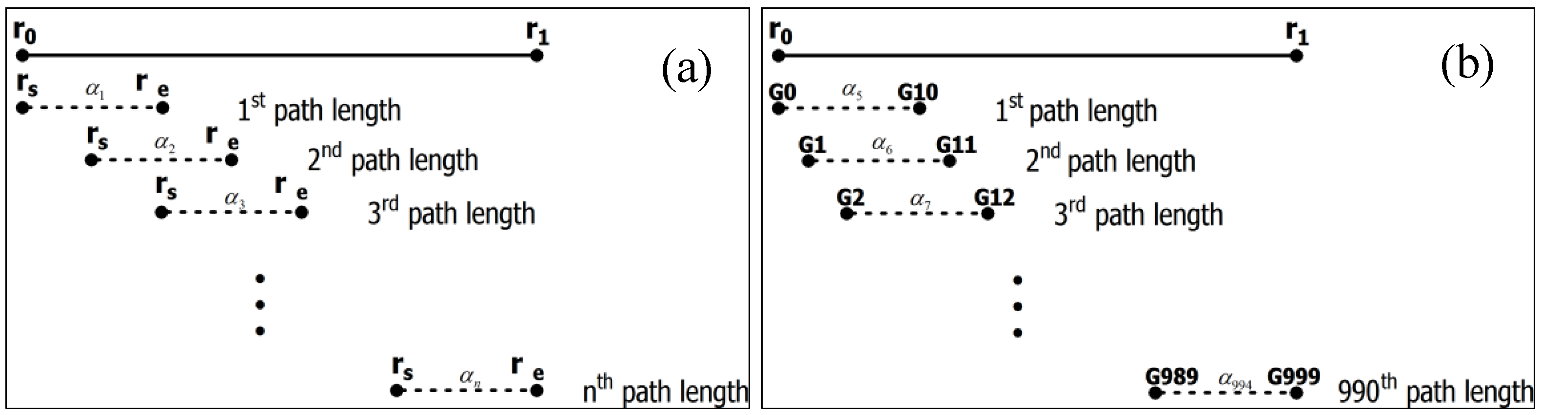
According to the scattering simulation results at X-band by Park et al. [27], α is set between 0.1 and 0.5, in a step of 0.03. Kim et al. [4] sets the distance between r₀ and r₁ as 1.0 km with an overlap of 0.5 km (ultimately, α has a resolution of 0.5 km), referring to Figure 1a. In the paper, the SSCC method employs a slide window processing shown in Figure 1b by setting the distance between r₀ and r₁ as 1.5 km (10 gates), thus α has a high-resolution of 0.15 km, improving the resolution of α estimation. After developing the method of Bringi et al. [3], Equations (3) and (10) become as follows:

$$\Delta {\mathsf{\varphi }}_{DP\_10gates}={\mathsf{\varphi }}_{DP}(G_{i+10})-{\mathsf{\varphi }}_{DP}(G_i)$$

(11)

$${\mathsf{\varphi }}_{DP\_10gates}^{error}(\mathsf{\alpha })={\displaystyle \sum _{i=0}^9\left|{\mathsf{\varphi }}_{DP}^{cal}(r_i;\mathsf{\alpha })-{\mathsf{\varphi }}_{DP}(r_i)\right|}$$

(12)

In addition, the new method does not seek the initial and terminal phase of each radial as the method of Bringi et al. [3] does, which would finally cause correction errors.

4. Result

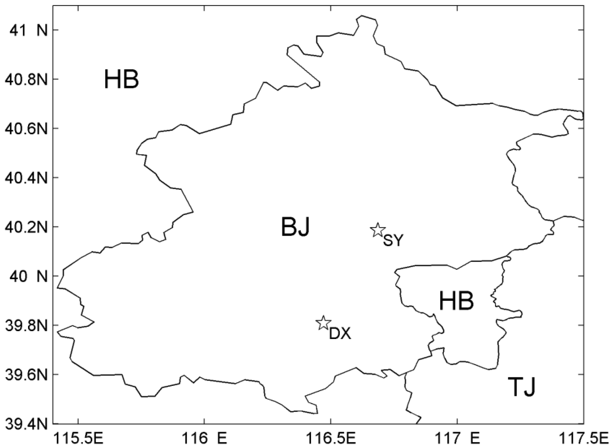
The SSCC method is evaluated using the data collected by the X-band dual-polarization radar (IAP-714XDP-A), which is located in Shunyi District of Beijing City (BJ) from June to September 2015. The data contain observations of convective cloud, stratiform cloud and the stratiform cloud with embedded convection. The corrected reflectivity is compared with the intrinsic reflectivity at X-band calculated from the reflectivity at S-band, which is obtained by the CINRAD/SA S-band single-polarization weather radar located in Daxing District of Beijing City. Figure 2 shows the locations of the two radars. The X-band radar (at ShunyiSY, 116.68° E, 40.19° N) is located at the northeast of the S-band radar (at DaxingDX, 116.47° E, 39.81° N). The straight-line distance between the two radars is about 46 km.

Hubbert and Bringi [31] pointed out that the measured differential propagation phase Ψ_C consists of true differential propagation phase φ_DP and backward scattering differential phase shift δ. Since δ could result in errors of K_DP estimation, δ needs to be eliminated before using Ψ_C. In this paper, the method of Hubbet and Bringi [31] is applied to filter δ out.

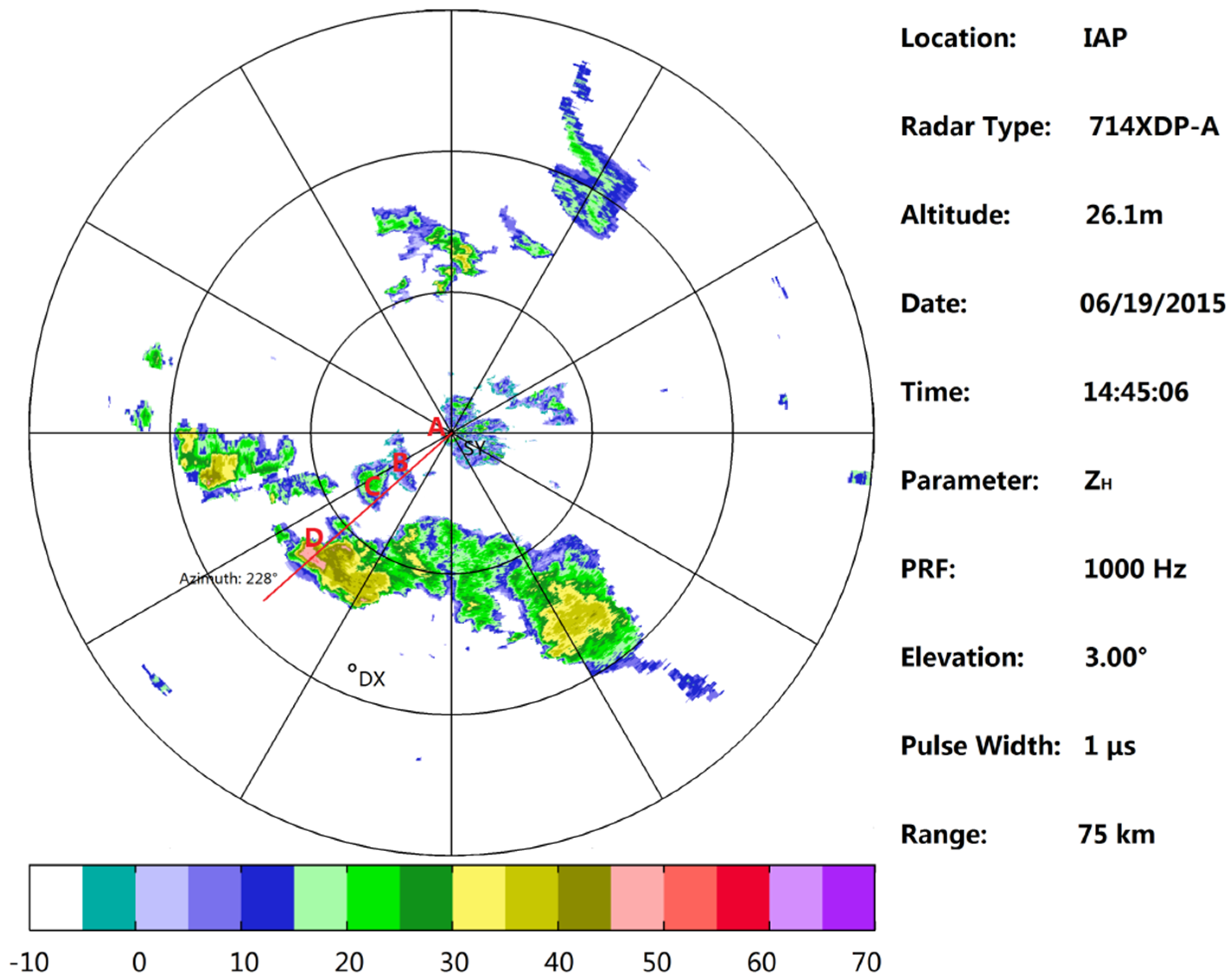
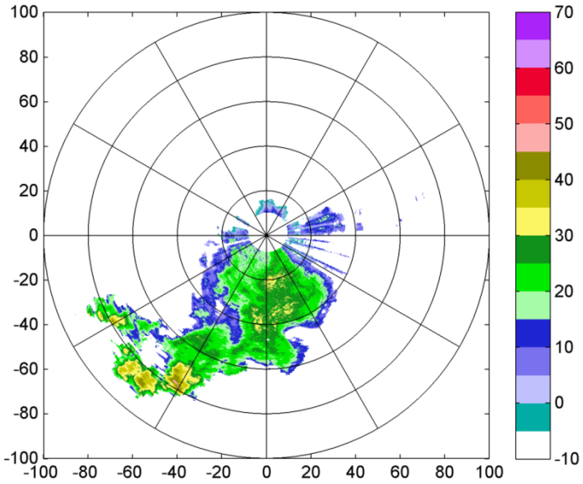
A strong convective weather event swept Beijing City from north to south on 19 June 2015. Figure 3 shows the plane position indicator (PPI) of the X-band radar at elevation 3° at 14:45 Beijing Time (BJT), 19 June 2015. Three strong echo cores of convective cloud are situated between the two radars and the largest reflectivity observed by the S-band radar is about 60 dBZ.

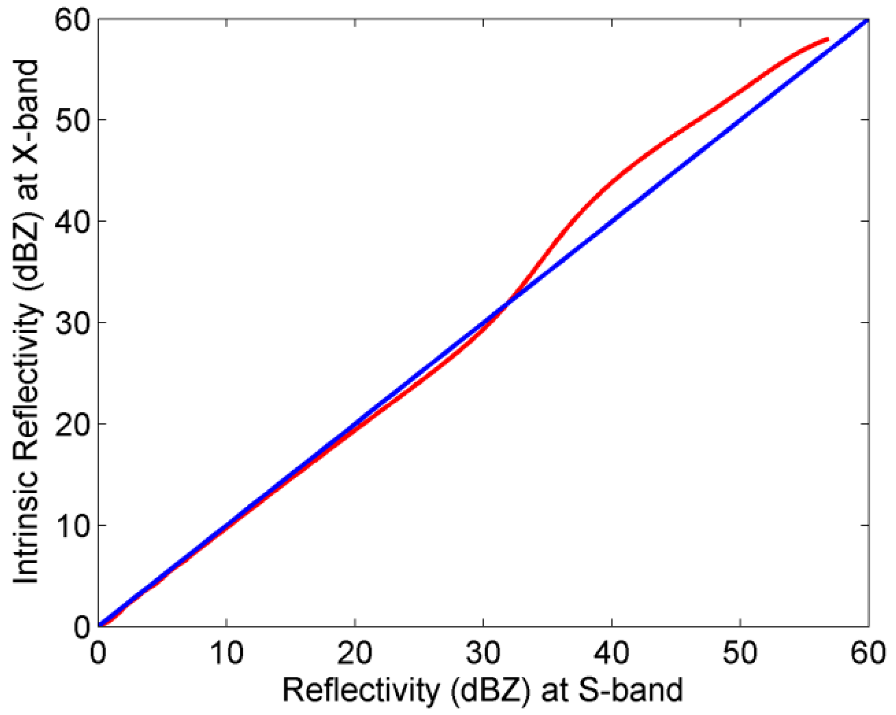
The intrinsic reflectivity at X-band is not equal to the reflectivity at S-band. Chandrasekar et al. [32] proposed three different methodologies for simulating X-band radar observations from the S-band radar data and the empirical conversion method is used in the paper. Figure 4 shows a plot of the intrinsic reflectivity at X and S bands for a monodispersed drop size distribution using the shape mode proposed by Beard and Chuang [33]. The relationship between the intrinsic reflectivity at X-band and the reflectivity at S-band is obtained by curve fitting, which is divided into three parts as shown in Equation (13) where subscripts X and S indicate simulated radar variables at X-band and measured radar measurements at S-band. Note that the reflectivity at S-band is assumed to be non-attenuated.

$$Z_{H,X}=\{\begin{array}{cc}0.9696Z_{H,S}-0.0145\hfill & \hfill Z_{H,S}\le 25dBZ\\ 1.1982Z_{H,S}-5.7726\hfill & \hfill 25dBZ<Z_{H,S}<45dBZ\\ 0.8206Z_{H,S}+11.7934\hfill & \hfill Z_{H,S}\ge 45dBZ\end{array}$$

(13)

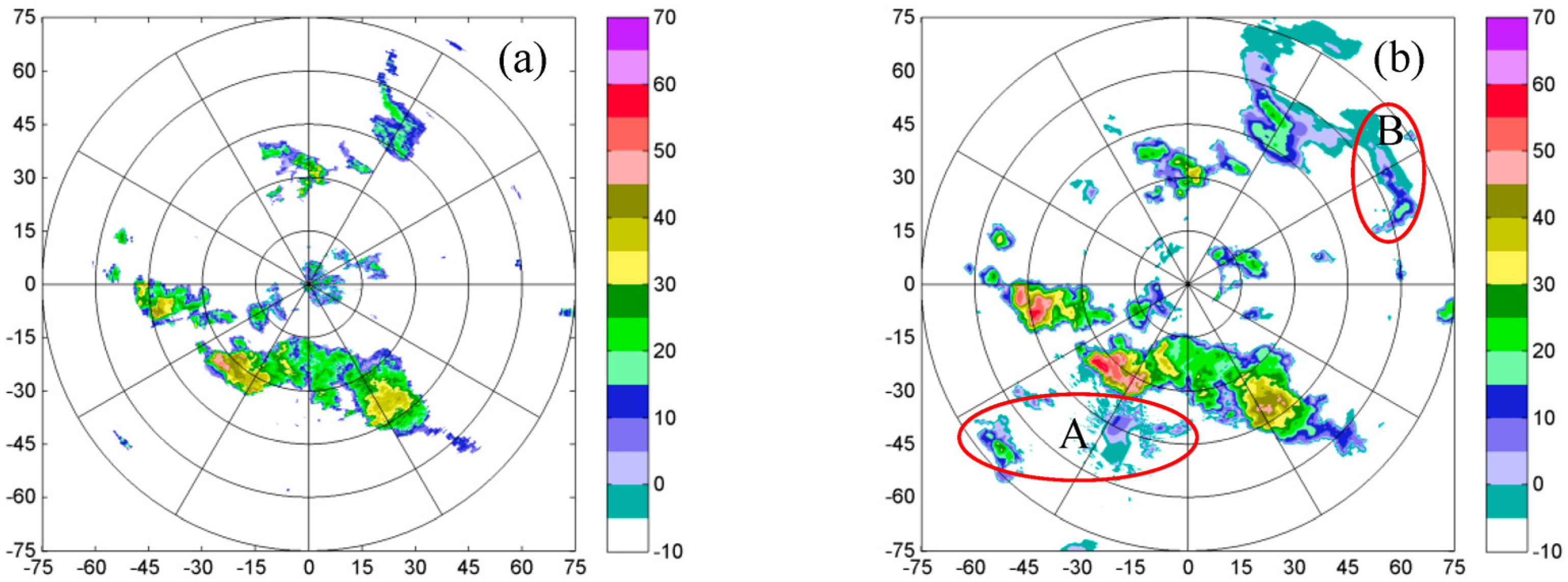
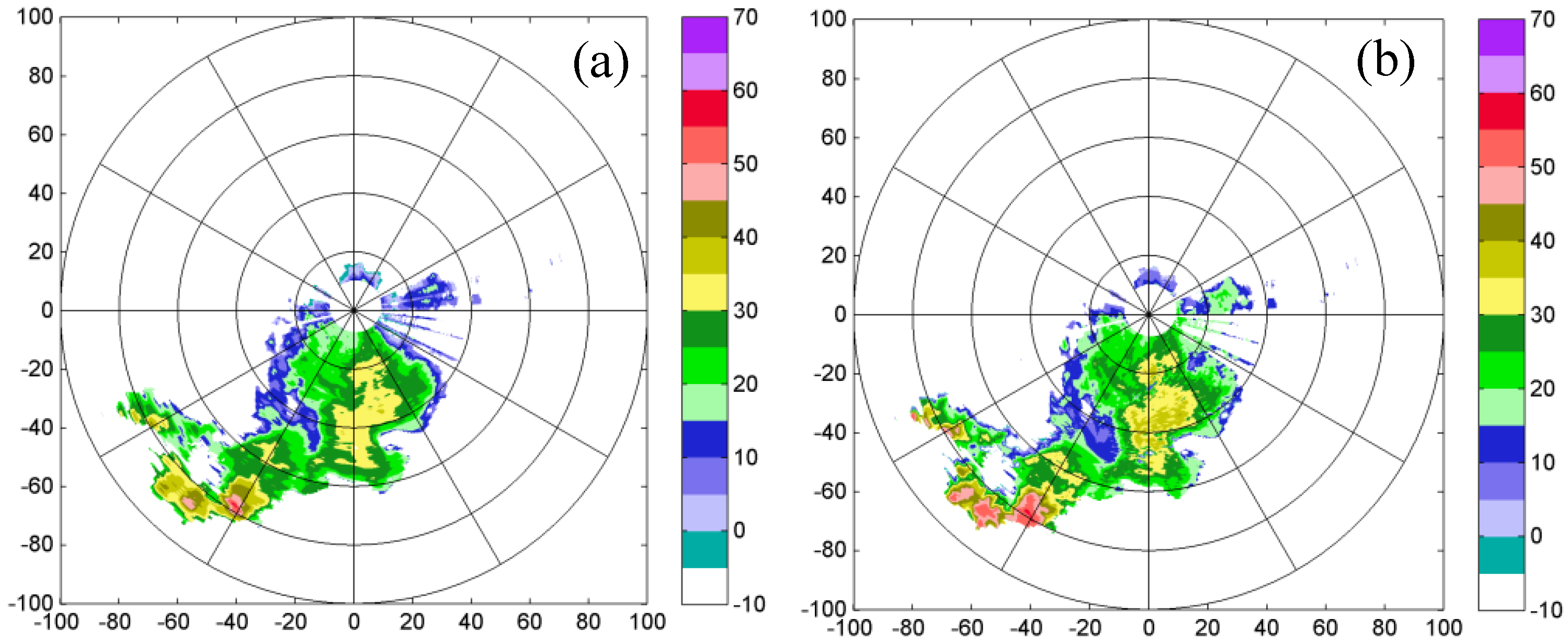
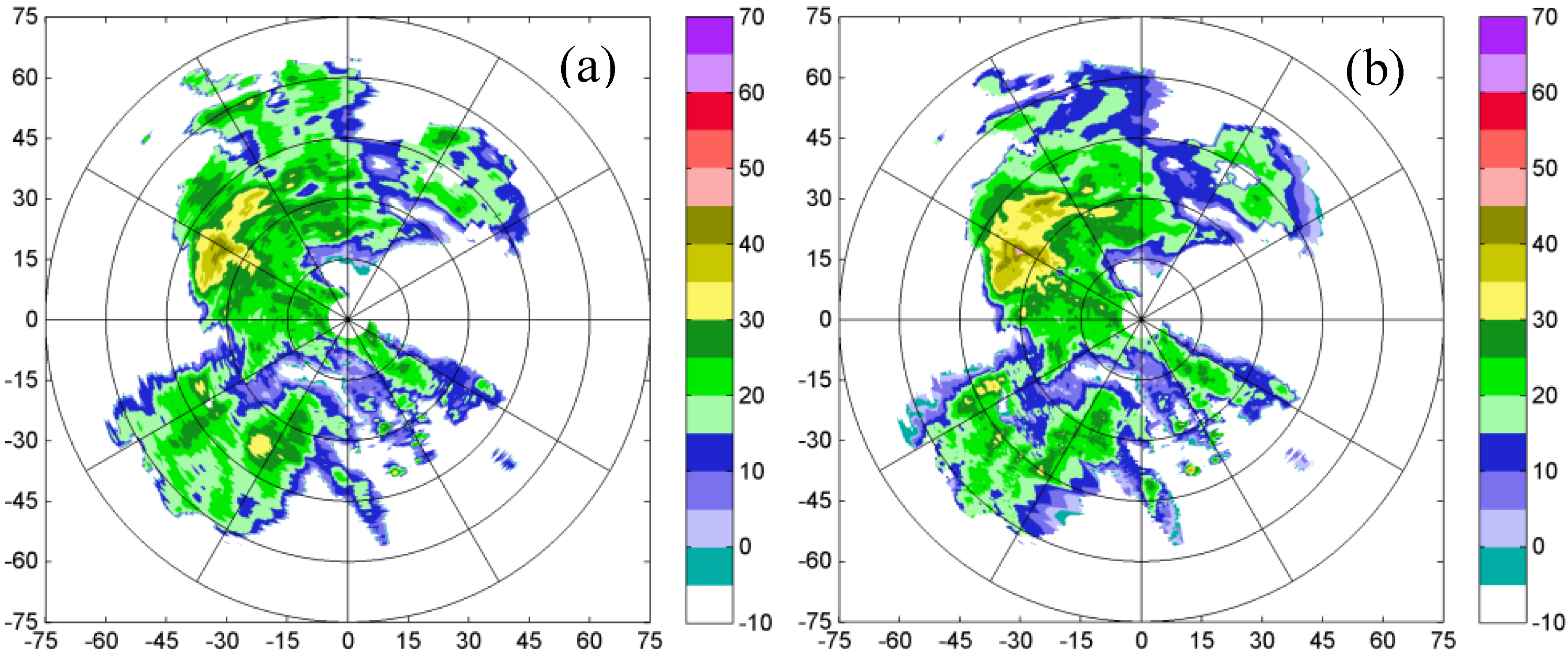
In order to analyze the accuracy of the SSCC method, the corrected X-band radar reflectivity is compared with the intrinsic reflectivity at X-band, which is calculated from the reflectivity at S-band. The S-band radar reflectivity from the volume scan data is interpolated into the coordinate of the X-band radar. The X-band radar PPI is shown in Figure 5a. Figure 5b is the intrinsic reflectivity at X-band. As shown in Figure 5a, there is a strong convective cloud band with three strong echo cores in the southwest of the X-band radar. Due to severe attenuation, the X-band radar cannot observe the echo after the intensive rain region, which is shown in circle A in Figure 5b. The echo of the circle B is also not be detected by the X-band radar, resulting from partial beam blockage.

The shapes of the two radar echoes are similar to each other, but the X-band radar reflectivity is seriously attenuated. The maximum reflectivity of convective cores at X-band is about 50 dBZ, while the corresponding intrinsic reflectivity is about 60 dBZ, indicating that the X-band radar echo has a serious distortion due to rain attenuation.

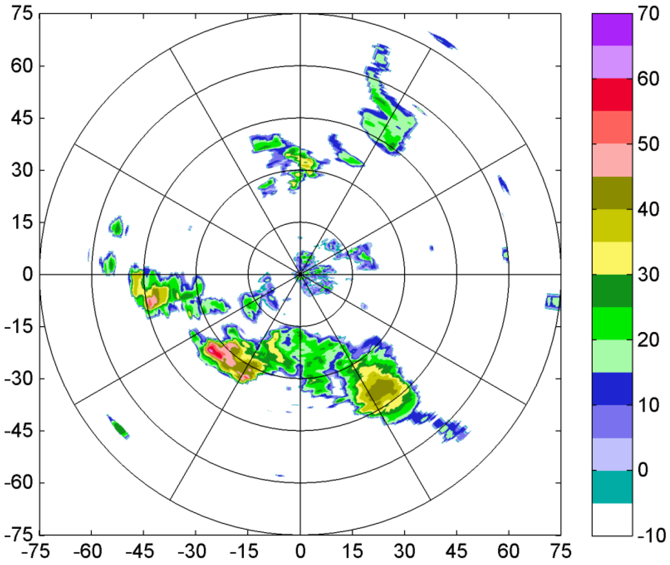
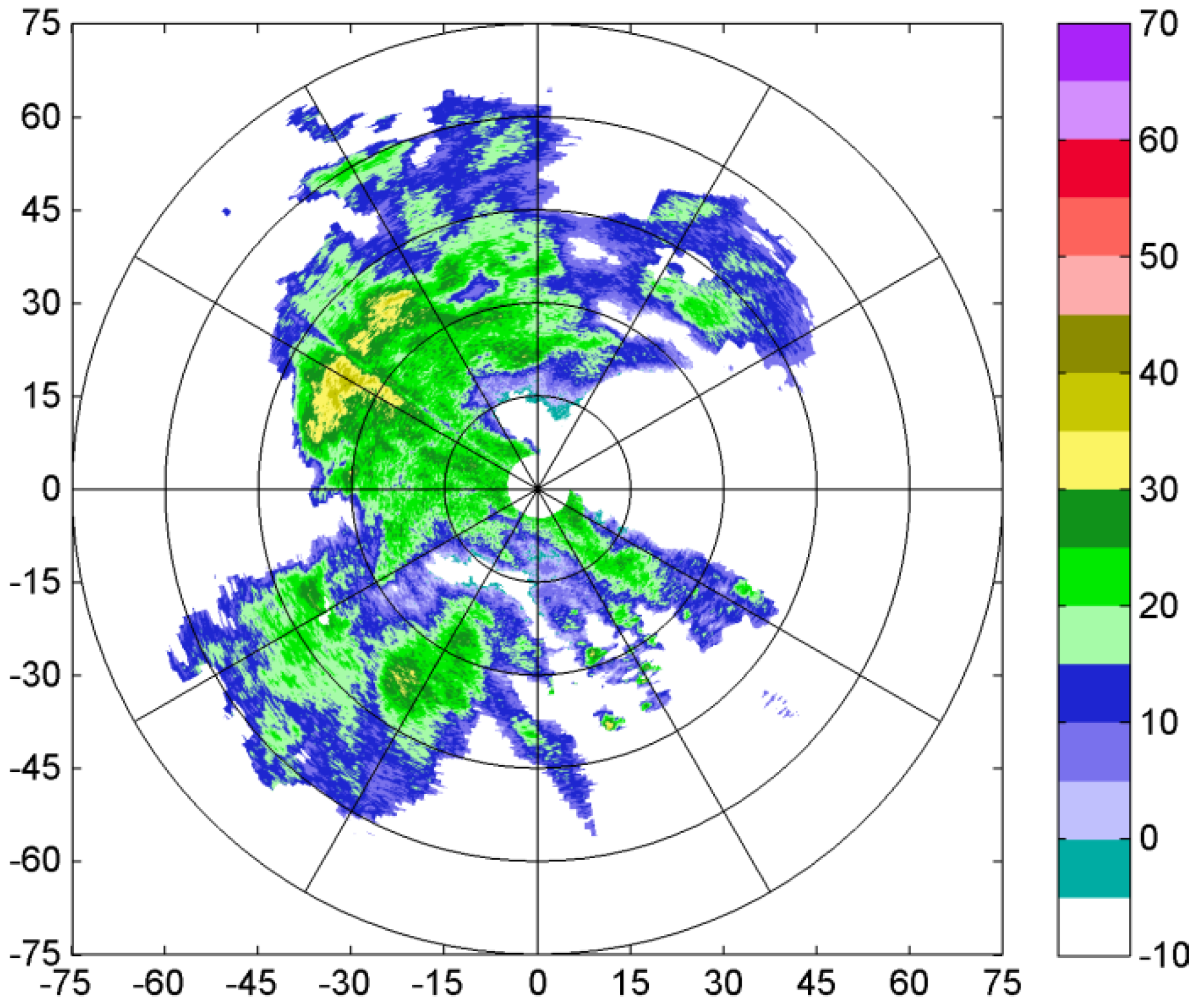
The reflectivity at X-band is corrected by the SSCC method, which is shown in Figure 6. Compared with the uncorrected X-band radar reflectivity in Figure 5a, the corrected reflectivity is effectively compensated and the scope of strong echois extended. For further analysis, the reflectivity is mapped into a 1000 × 1000 matrix grids with a resolution of 150 m.

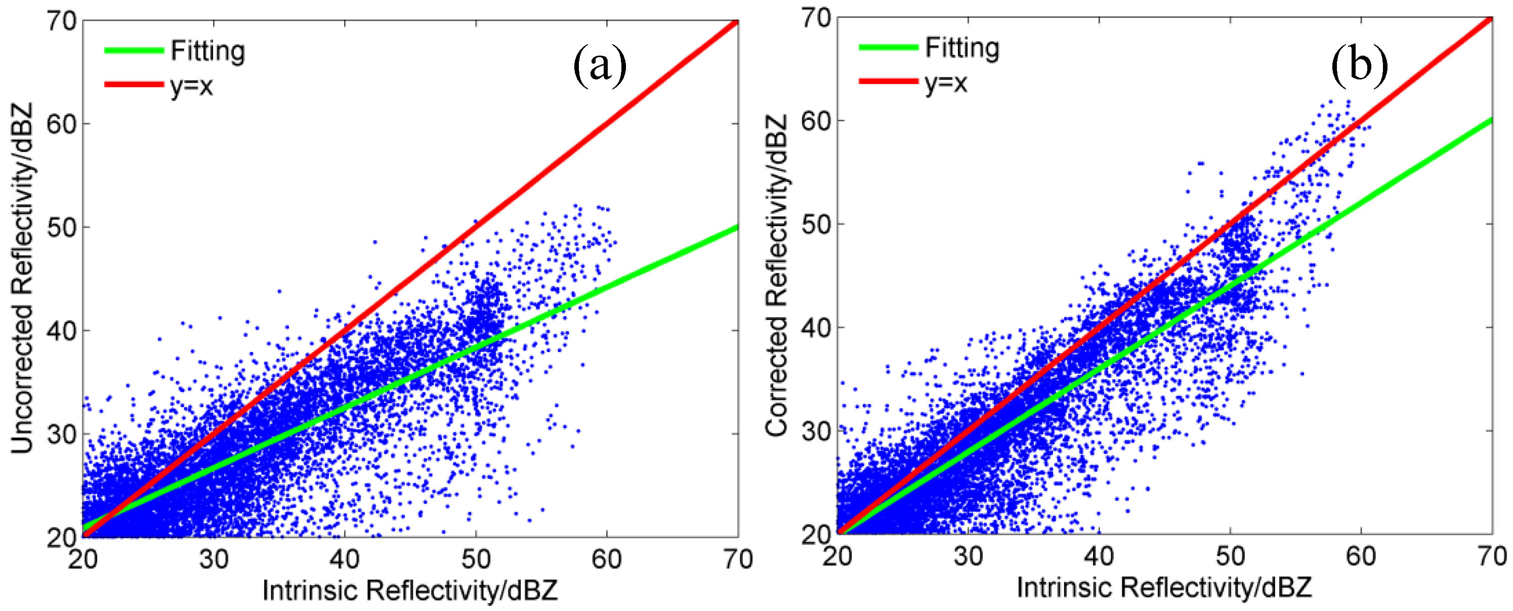
Figure 7 shows the scatter diagrams of the uncorrected and corrected X-band radar reflectivity versus the intrinsic reflectivity. Figure 7a shows that the uncorrected reflectivity significantly deviates from the intrinsic reflectivity, especially when the echoes are strong. The fitting line between the uncorrected reflectivity and the intrinsic reflectivity (the green line) is y = 0.5824x + 9.2234, while the fitting line between the corrected reflectivity and the intrinsic reflectivity becomes y = 0.8036x + 3.8382, referring to Figure 7b. After attenuation correction, the slope of fitting line turns 0.5824 into 0.8036, indicating that the corrected reflectivity is much closer to the intrinsic reflectivity.

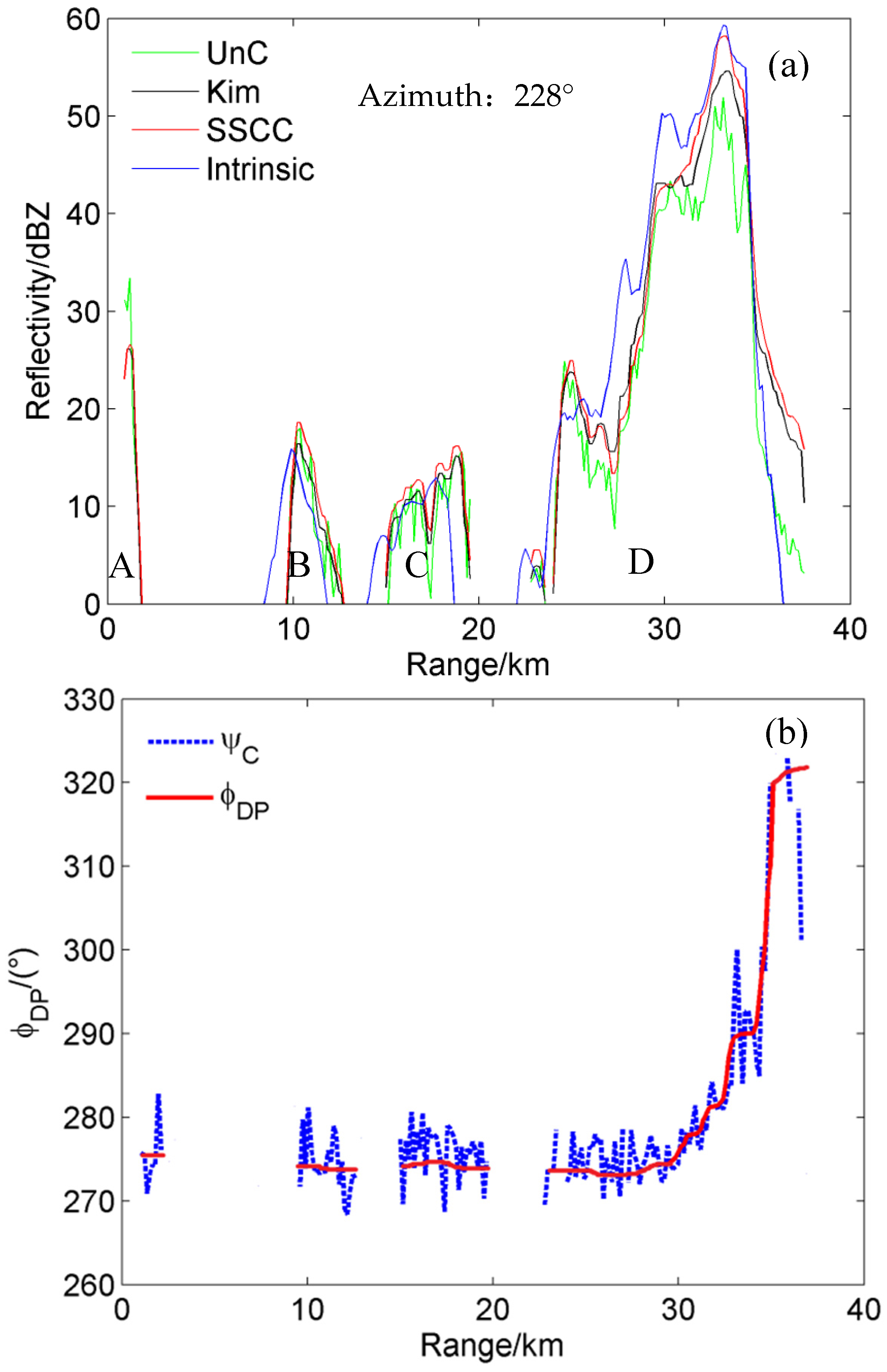
In order to show the validity of the correction for any path, the reflectivity at X-band with an azimuth angle of 228° is analyzed herein. As shown in Figure 3, the electromagnetic wave successively passes from A to D. Due to the impact of distance, antenna elevation and earth curvature, there are not echoes of the S-band radar in the area A, referring to Figure 8a. Compared with the intrinsic reflectivity (Intrinsic), the uncorrected reflectivity (UnC) nearly has no attenuation in areas A, B and C while with serious attenuation in area D. Figure 8b also illustrates this phenomenon, the φ_DP increases by nearly 50°, corresponding to intensive rain region, while no increase in areas A, B and C. After attenuation correction using the SSCC method, the corrected X-band radar reflectivity at 33 km has compensated about 10 dBZ (SSCC). The corrected reflectivity at X-band is consistent with the intrinsic reflectivity. However, the corrected reflectivity using the method of Kim et al. [4] (Kim) is lower than the intrinsic reflectivity, indicating the correction is not enough.

The corrected X-band radar reflectivity at 37 km in Figure 8a is 15 dBZ larger than the intrinsic reflectivity. This results from the rapid development and fast moving speed of the convective cloud. Because the intrinsic reflectivity shown in Figure 5b is interpolated by the 6-min volume scan data of the S-band radar, the two factors causes a slight deviation from the intrinsic reflectivity. This influence is significant at the edge of convective cloud but negligible for the stratiform cloud and the stratiform cloud with embedded convection. As shown in Figure 8a, the corrected X-band radar reflectivity both the SSCC and the Kim is close to the intrinsic reflectivity. However, the SSCC method has an advantage over Kim et al. [4] in correcting the reflectivity of the convective cloud. In order to analyze the two methods comprehensively, all the radials are used.

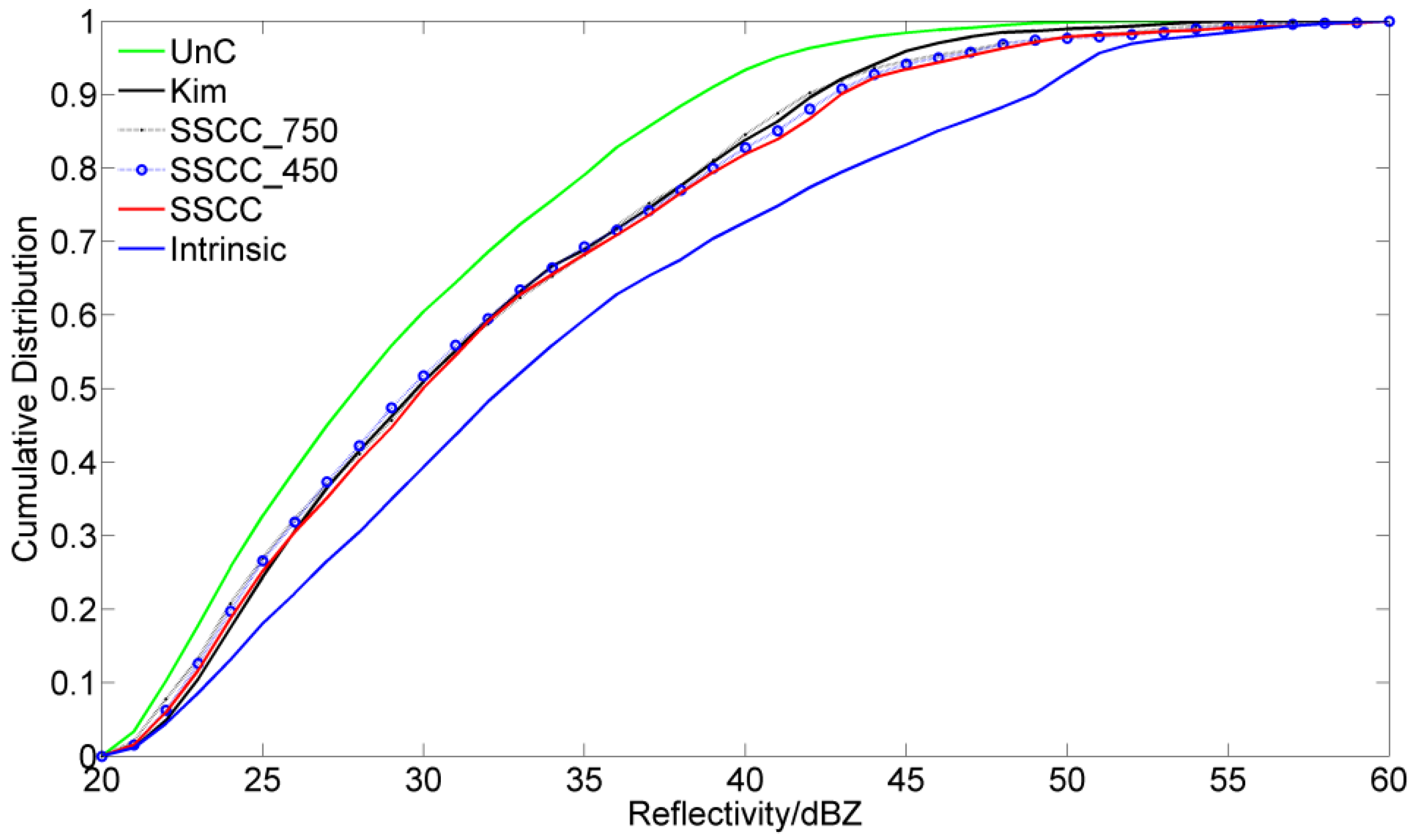
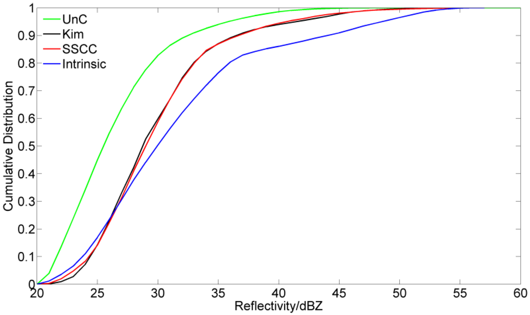
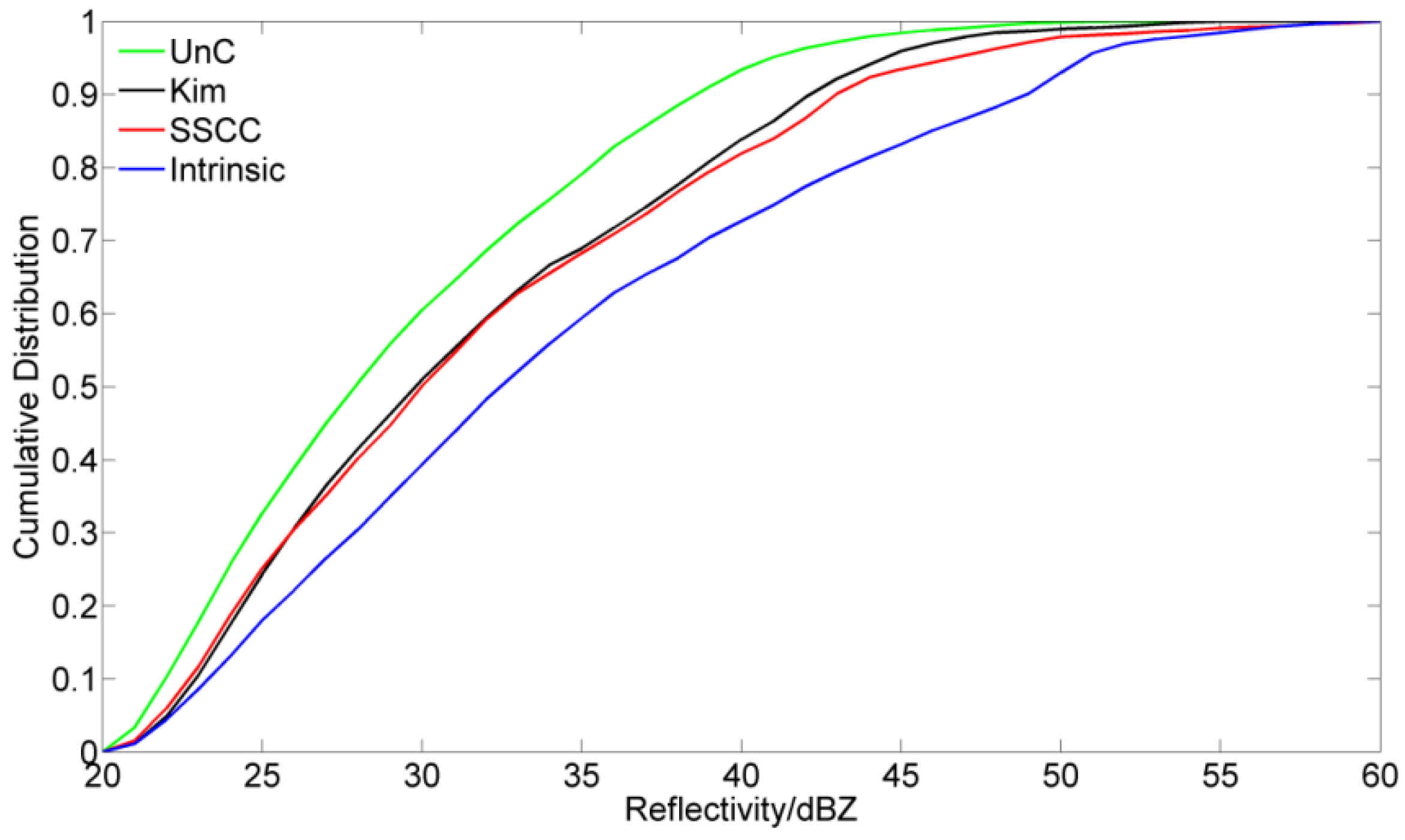
Figure 9 shows four cumulative distributions of the radar reflectivity. Comparing with the cumulative distribution of the uncorrected reflectivity (UnC), the method of Kim et al. [4] (Kim), and the SSCC method (SSCC) both shift to the right, indicating that the low cumulative value of reflectivity decreases, while the high cumulative value increases. Both the cumulative distribution of the Kim and SSCC are closer to that of the intrinsic reflectivity than the UnC. The average biases (AB) of the reflectivity are calculated for the two methods.

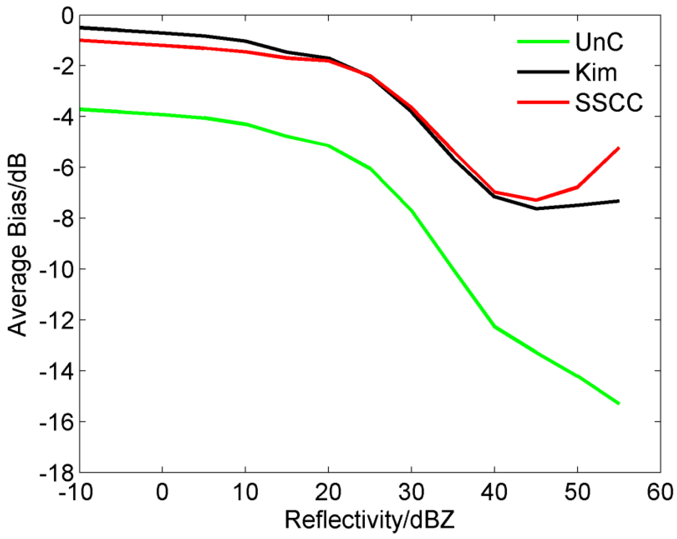
The average bias (AB) shown in Figure 10 is defined as below:

$$AB=\langle R-R_s\rangle {|}_x$$

(14)

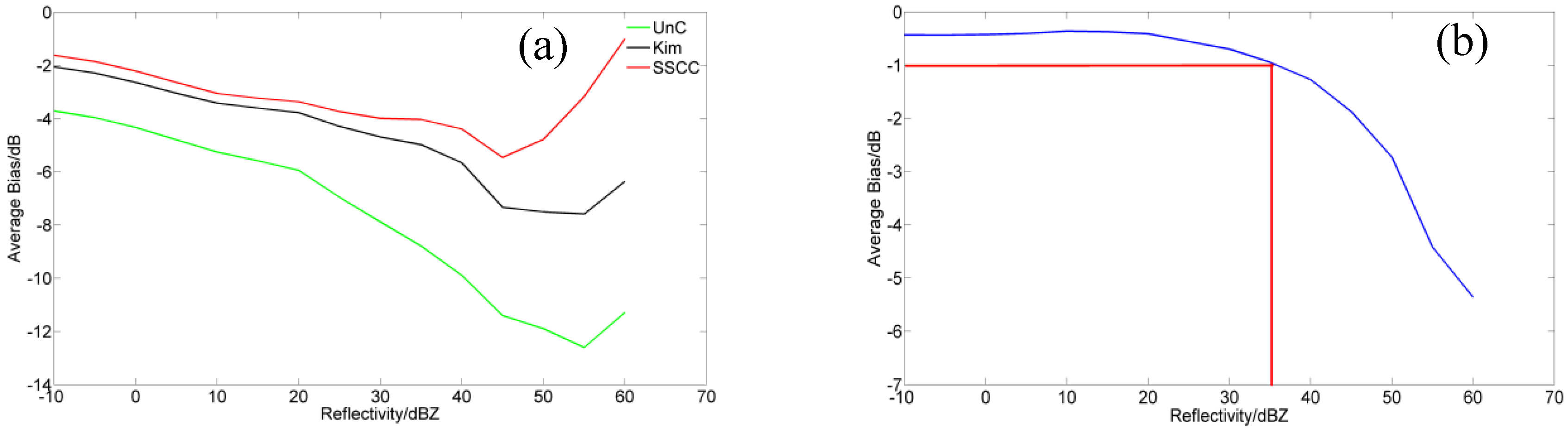
where $\langle \ast \rangle {|}_x$ is average value above parameter x, R is the reflectivity at X-band and R_S is the intrinsic reflectivity. As shown in Figure 10a, the AB between the uncorrected reflectivity and the intrinsic reflectivity (line UnC) is decreasing with increasing reflectivity. The AB of the UnC is greater than 10 dB, indicating that the attenuation is significantin the rain area. The AB of the Kim and SSCC significantly reduces the difference from the intrinsic reflectivity. To accurately retrieve meteorological products, a resolution of 1 dB for the reflectivity is necessary. Figure 10b shows that there are more than 1 dB differences between the Kim and SSCC from 35 dBZ, illustrating that the SSCC method has a better performance than Kim et al.’s method at correcting convective cloud, especially with reflectivity greater than 35 dBZ.

In order to analyze the impact of different sampling resolutions for the SSCC method, the range resolution is set at 0.45 km (SSCC_450) and 0.75 km (SSCC_750) as shown in Figure 11, respectively. The SSCC_750 is further away from the Intrinsic than the SSCC_450, which is closer to the method by Kim et al. [4] (the range resolution is 0.5 km). Figure 11 shows that the decreasing range resolution would lead to reduced correction effect and the SSCC method performs better than the method by Kim et al. [4] for convective cloud.

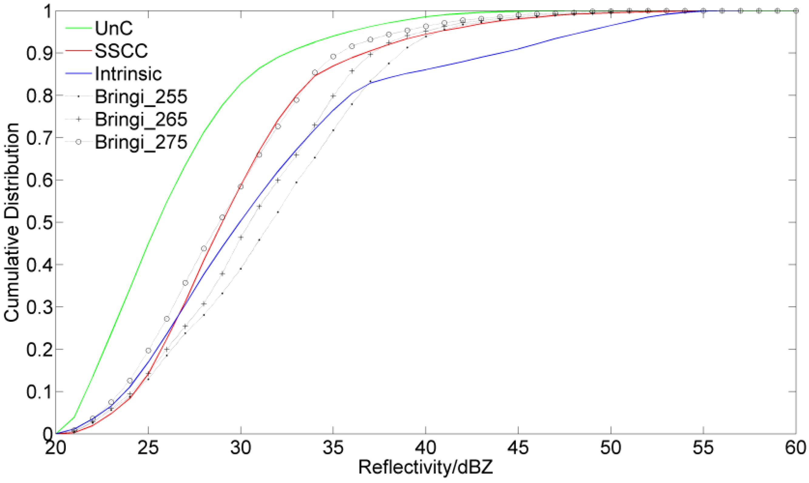
Compared with the method by Bringi et al. [3], the SSCC method does not require an initial and a terminal differential propagation phase of each radial, which could avoid correction errors. To illustrate this problem, we assume the terminal phase is true and examine the errors due to the wrong initial phase. Figure 12 shows correction errors with various initial phases using the method by Bringi et al. [3], whereby 275° (Bringi_275) is the actual radar initial phase and 255° (Bringi_255) and 265° (Bringi_265) are not. The SSCC is consistent with the Bringi_275. In contrast, the Bringi_255 and the Bringi_265 are far away from the Bringi_275, indicating the SSCC method does not require seeking the initial phase and terminal phase but the cumulative distribution is also consistent with that of the true correction results.

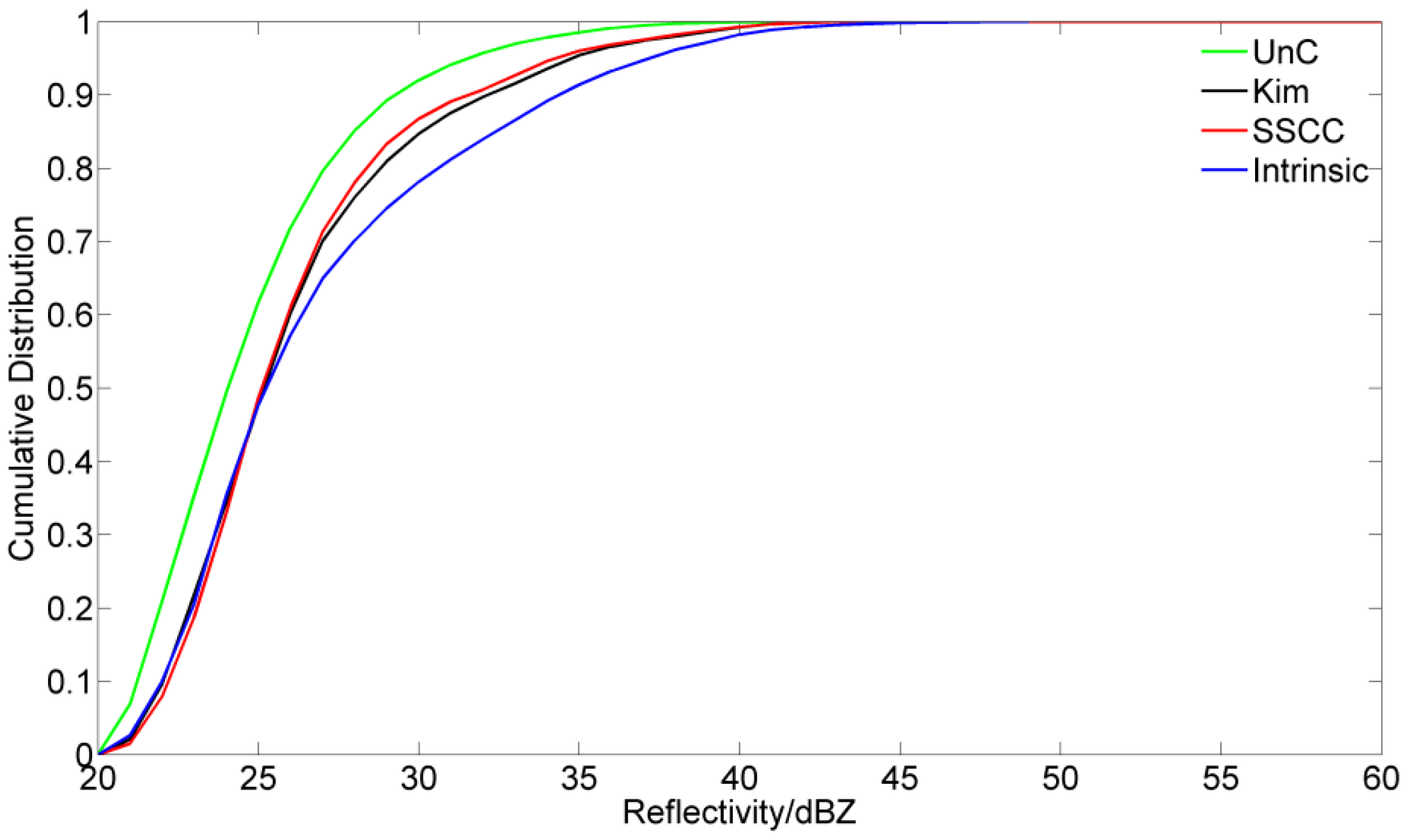
To verify the applicability of the SSCC method under various precipitation conditions, the stratiform cloud with embedded convection on 26 June 2015 (Figure 13 and Figure 14), and the stratiform cloud on 16 June 2015 (Figure 15 and Figure 16) are analyzed. Both Figure 17 and Figure 18 show that the reflectivity at X-band is corrected effectively and the corrected cumulative distribution closer to that of the intrinsic reflectivity. Figure 19 and Figure 20 show that the SSCC method is consistent with the method by Kim et al. [4]. The change of the resolution does not lead to correction biases, because the K_DP of the stratiform cloud with embedded convection and the stratiform cloud is lower than that of the convective cloud. Figure 21 and Figure 22 illustrate that the corrected cumulative distribution using the SSCC method are consistent with that of the 275°, which is the true initial phase of the radar. The correction verification of the three different precipitation cases indicates that the SSCC method is also applicable for the stratiform cloud and the stratiform cloud with embedded convection. Note that both the SSCC method and the method by Kim et al. [4] may have no significant effect or lead to slightly worse attenuation correction due to the error of the integration resolution when correcting stratiform rain if the rainfall is very small.

5. Conclusions and Discussion

Based on Bringi et al. [3], the paper proposed a high-resolution slide self-consistency correction (SSCC) method for the X-band dual-polarization radar reflectivity, which is an improvement from Kim et al.’s method. The proposed method improved the correction resolution and effect, adapting a slide window consisting of 10 gates.

In the paper, the SSCC method is evaluated with the reflectivity of the convective cloud, the stratiform cloud with embedded convection and the stratiform cloud, comparing with the correction results from the methods by Bringi et al. [3] and Kim et al. [4], as well as the intrinsic reflectivity at X-band calculated from the reflectivity at the S-band. It is found that the reflectivity at X-band can be corrected effectively by the SSCC method. The corrected reflectivity is closer to the intrinsic reflectivity and has a better performance than the method by Kim et al. [4] in correcting the convective cloud. However, the correction results of the two methods are very similar for the stratiform cloud with embedded convection and the stratiform cloud. This may be because the K_DP of the two kinds of precipitation cloud is much less than that of the convective cloud. For this reason, the SSCC method and the method by Kim et al. [4] may have no significant effect or may lead to slightly worse attenuation correction when correcting stratiform rain if the rainfall is very small. In addition, the SSCC method has better results than Bringi et al. [3] for the three cases due to the reduced correction errors when computing differential propagation shift increments.

In summary, the SSCC method has three advantages as follows:

• Improving the correction resolution;
• Having no need for seeking the initial and terminal differential phases;
• Good performance in correcting convective cloud.

Meanwhile, it must be noted that the accuracy of the attenuation correction is restricted in the SSCC method by the length (1.5 km) of the sliding window and this is a more significant effect than the resolution.