1. Introduction
Lightning return-stroke models have been categorized by Rakov and Uman [
1] into four classes depending on their governing equations: (a) gas dynamic models; (b) engineering models; (c) distributed circuit models; and (d) electromagnetic (or antenna-theory) models.
Among these categories of models, the electromagnetic models have received increased attention in the past few years (e.g., [
2]), partly because of wider availability of full-wave numerical codes and increased computer capabilities [
3]. In electromagnetic models, Maxwell’s equations are solved to obtain the current distribution along the lightning return-stroke channel (considered as an antenna), and on neighboring metallic structures such as towers, buildings, and overhead or underground transmission lines. Different numerical techniques are used in electromagnetic models, namely integral equation (IE)-based methods (such as the method of moments), or differential equation (DE)-based methods (such as finite difference time-domain (FDTD)) methods in the time or the frequency domain. Baba and Rakov [
4,
5] provided a classification of the electromagnetic models in terms of the channel representation, the excitation method, and the employed numerical technique.
In electromagnetic models, the return-stroke channel is generally represented as an antenna excited at its base by either a voltage or a current source. The speed of the current pulse propagating along a vertical antenna in free space is nearly equal to the speed of light. This is in contrast with optical observations on lightning return strokes, which suggest that the return stroke speed is lower typically in the order of one third to one half of the speed of light [
6], although there is some controversy as discussed below. The current wave speed along the channel is commonly assumed to be the same as the optical speed. Based on Maxwell’s equations coupled with air plasma thermodynamics equations, Liang et al. [
7] presented numerical simulations suggesting that the current speed is much higher than the optical speed and is in the order of 80% to 90% of the speed of light. On the other hand, Carvalho et al. [
8] reported measured values of current-to-luminosity delays based on simultaneous experimental records of lightning channel-base currents and their associated luminosity for 22 return strokes in eight Florida triggered lightning flashes. The measured delays were found to be significantly shorter that that predicted by Liang et al. [
7] from their theory. Note also that the relation between the return stroke and the optical speeds can also be affected by the shape of the channel. The channel tortuosity and channel inclination have been considered in several studies (see, e.g., Section VIII. C of [
1]).
In this paper, we have considered return stroke current speeds ranging from 1.3 × 10
8 m/s to 2 × 10
8 m/s, corresponding to typical optically measured values. It is worth noting, however, that the parameters of the models can also be adjusted to reproduce higher speeds as predicted by Liang et al. [
7].
Different representations for the return-stroke channel have been proposed in the literature in which different techniques have been used to artificially reduce the propagation speed of the current pulse down to values compatible with optical observations. Baba and Rakov [
9] presented a comparison between available representations of the return-stroke in electromagnetic models which included:
A wire embedded in a fictitious half-space dielectric medium (other than air) [
5,
10].
A wire with a fictitious dielectric coating (other than air) [
5].
A wire in free-space loaded by distributed series inductance [
5,
11].
Two parallel wires in free-space having additional distributed shunt capacitance [
5,
12].
In the analysis presented in [
9], the two-dimensional FDTD technique was used to simulate the predictions of the considered electromagnetic models. The main conclusion of [
9] was that the two representations with distributed series inductance and fictitious dielectric coating were able to reproduce the maximum number of characteristic features of measured electromagnetic field waveforms. Furthermore, they showed that modifications of these two representations including a height-dependent distributed resistance can reproduce all the experimentally observed features.
To the best of our knowledge, the FIT-based method has not been used to model the return stroke channel in the past. In this paper, we will present an analysis of the electromagnetic models in terms of their practical implementation using a time-domain method based on the finite-integration technique (FIT). The FIT-based methods use local operators (leading to sparse matrices [
13,
14]) and volumetric discretization of the whole computational domain, and they require an absorbing boundary condition to truncate the domain.
The FIT-based solvers have many of the same advantages of FDTD-based solvers, such as simple implementation and efficiency for parallel computing. Some of the FDTD-based solvers, however, suffer from disadvantages that are compensated for by using FIT. For example, FIT uses finite-volume type discretization of Maxwell’s equations, which leads to Faraday’s law being satisfied within each mesh-cell and in the whole the computational domain. In this sense, FIT allows to prove conservation properties of discrete fields in an inhomogenous medium [
15].
The main objective of the present paper is to provide a systematic comparison between different electromagnetic models in terms of their practical implementation. The presented analysis is different from the earlier work of Baba and Rakov [
2,
4,
5], in which the review of electromagnetic models was carried out with an emphasis on their applications (strikes to flat ground, strikes to free-standing objects, strikes to overhead power lines, and strike to wire-mesh-like structures) and their ability to reproduce typical values of optically measured return-stroke wavefront speed, the equivalent impedance of the lightning return-stroke channel, and the remote electric and magnetic fields is discussed.
In the present paper, we use the same classification of the electromagnetic models proposed by Baba and Rakov, but the focus is on their practical implementation, rather than their scope of applications and their ability to reproduce the main features of radiated electric and magnetic fields.
Criteria used for the analysis are as follows:
Ease of implementation of the model.
Numerical accuracy of the model.
Efficiency of the model (computational time and memory requirements).
Ability to reproduce a desired value for the speed of the current pulse.
The rest of the paper is organized as follows. In
Section 2, the current distribution along the lightning channel is calculated using CST-MWS for different electromagnetic models. In
Section 3, we provide a discussion on the implementation of each model, including their numerical accuracy, computational time and memory requirements, as well the required conditions to reproduce the desired value for the return-stroke speed. Conclusions are presented in
Section 4.
2. Current Distribution along the Lightning Channel for Different Electromagnetic Models
In this section, the current distributions along the lightning channel for different electromagnetic models are calculated using CST-MWS.
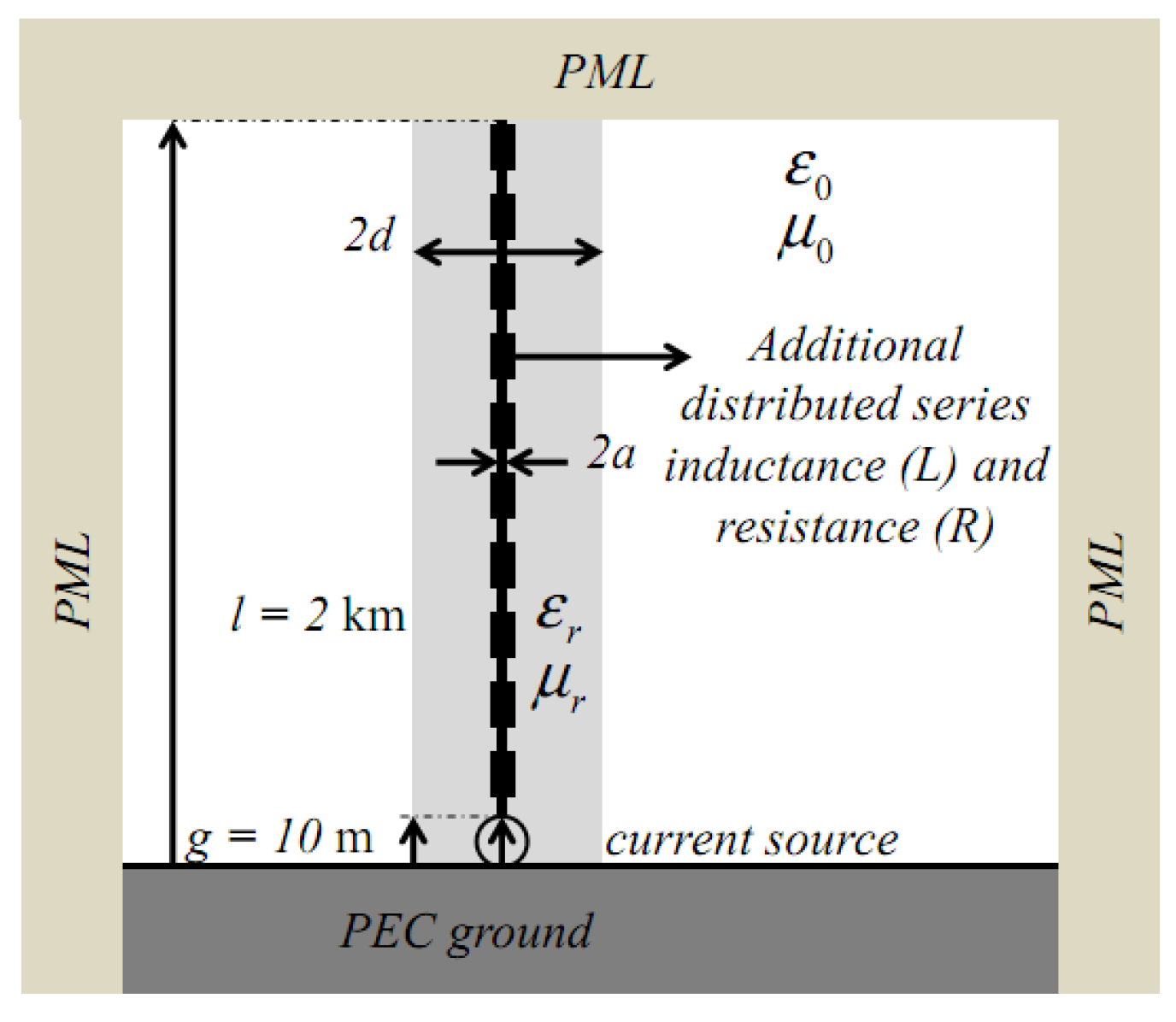
Figure 1 shows a generic representation of the lightning return-stroke channel as used in various representations of electromagnetic models with the aim of reducing the propagation speed of the current pulse. The model consists of a vertical thin wire monopole antenna with a fictitious dielectric coating over a flat PEC ground, excited at its base by a lumped current source. In this figure,
a,
d,
l, and
g denote the radius of the wire, the thickness of the fictitious dielectric coating surrounded by air, the length of the lightning channel and the lumped current source length, respectively. The return-stroke channel can be loaded by additional distributed series resistance
R, and inductance
L, as shown in
Figure 1.
We will present simulations for the following available representations of the electromagnetic models:
- -
Model A: A wire embedded in a fictitious half-space dielectric medium (other than air).
- -
Model B: A wire embedded in a fictitious dielectric coating with permittivity (εr) and permeability (μr).
- -
Model C: A wire in free-space loaded by distributed series inductance and resistance.
The used lumped current source at the channel base injects a typical subsequent return stroke current characterized by a peak value of 12 kA and a maximum steepness of 40 kA/μs, represented by a sum of two Heidler’s functions whose parameters can be found in [
16]. In all simulations in CST-MWS, the mesh cells are optimized based on the thin-wire antenna to reduce the memory resources and computational time [
14]. All the presented simulations were carried out on a personal computer with Intel 2.30 GHz Dual-Core processors with 4 GB RAM.
2.1. A Wire Embedded in a Fictitious Half-Space Dielectric Medium (Model A)
In this case, with reference to
Figure 1, the return-stroke channel is modeled as a thin-wire monopole antenna of radius
a = 0.23 m embedded in a half-space dielectric medium (
d =
) with a relative permittivity
εr (
μr = 1.0). The lightning channel is not loaded by any distributed series resistance or inductance (
R = 0,
L = 0).
In CST-MWS simulations, the flat PEC ground was modeled by a square plate of dimension 10 × 10 m
2 located in the
x-
y plane. The return-stroke channel is considered as a thin cylindrical PEC above the flat ground. A discrete, 10-m long port is placed between the flat ground and the thin-wire lightning channel as a lumped current source. To monitor the current waveform along the lightning channel, three lumped elements (10
−5 Ω-resistance) are used at heights 150 m, 300 m, and, 600 m along the return-stroke channel. The current distribution along the channel is virtually unaffected by the presence of these lumped elements. To truncate the computational domain in CST-MWS, a perfectly matched layer (PML) is set on the four lateral surfaces, as well as on the top surface of the structure (see
Figure 1). The bottom surface is assumed to be a PEC surface. Due to the problem symmetry, in this simulation we can use two symmetry planes in CST-MWS to reduce the computational time and memory resources. The adopted time step and the number of time steps are 9.75 ns and 5128, respectively. The frequency range for this example is 0–2 MHz.
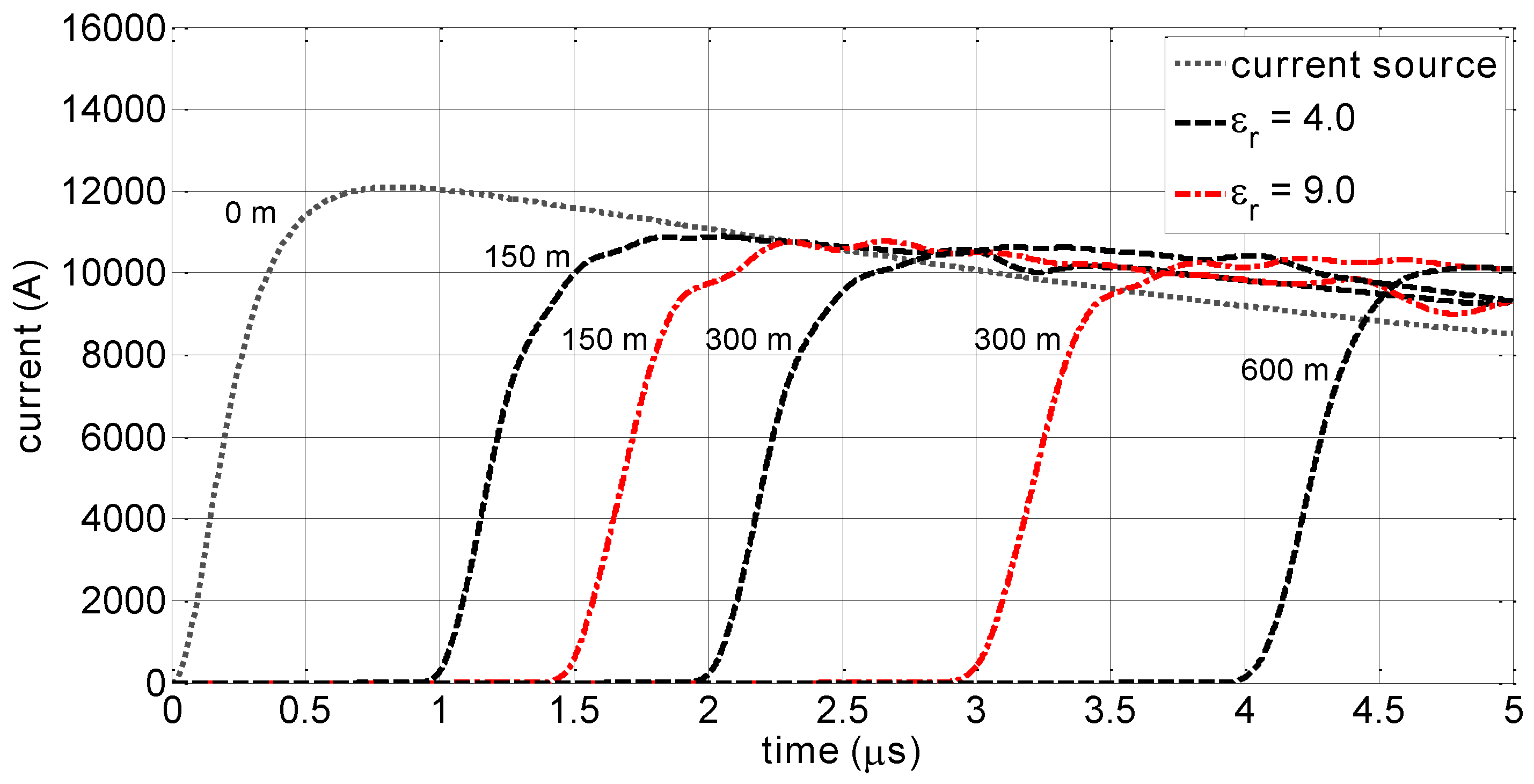
Figure 2 shows the CST-MWS-calculated current distribution along the return-stroke channel modeled as a PEC thin-wire embedded in a half-space dielectric for two values for the relative permittivity,
εr = 4 and 9. As expected, this representation results in a propagation speed of the current pulse along the channel of
, where
εr and
c denote the relative permittivity of the half-space dielectric and the velocity of light in free space, respectively. For
εr = 4 and
εr = 9, the resulting propagation speeds are about 0.5
c and 0.33
c, respectively. Increasing the value of the relative permittivity reduces the wavelength, which leads to a higher number of mesh cells and, in turn, to an increase in memory resources and computational time. Note that, throughout this paper, the speed of the current pulse along the channel is calculated on the basis of the time needed for current waves to propagate along the channel from the channel base to 150 m, determined by tracking the intersection point between a straight line passing through the 10% and 90% points on the rising part of the current waveform and the time axis.
Table 1 shows the computational time and memory resources that are needed for the CST-MWS simulation for the mentioned example with and without symmetry planes. Using two symmetry planes, the memory resources and computational time can be reduced by a factor of 2 and a factor of 4, respectively.
The main drawback of this electromagnetic return-stroke model is that, once the current along the channel has been calculated, it requires a second step for the calculation of the generated electromagnetic field with the dielectric removed.
2.2. A Wire with a Fictitious Coating with εr and μr (Model B)
In this model, the lightning channel is modeled by a vertical thin-wire monopole antenna embedded in a dielectric coating with a square cross section of dimension 2d × 2d m2. The coating is characterized by a relative permittivity εr and a relative permeability μr.
Similar to the previous model, the return-stroke was represented as a PEC thin-wire of radius
a = 0.23 m above a 10 × 10 m
2 PEC ground plane. A discrete, 10 m long current port is placed between the flat ground and the lightning channel. The excitation signal used was that of a typical return-stroke represented by Heidler’s functions [
16]. As with the model in the previous section, three lumped elements were used at heights 150 m, 300 m, and 600 m along the thin-wire to monitor the current waveform along the lightning channel. The simulation conditions were the same as those in the model of the previous subsection: the computational domain was truncated by a PML set on the four lateral surfaces and on the top surface of the structure, a PEC was used for the bottom surface, and two symmetry planes are used to reduce the computational time and memory resources.
It should be noted that in Model B1 the coating is only characterized by a relative permittivity εr (the relative permeability μr is equal to 1) while in Model B2, the coating is represented by a relative permittivity εr and a relative permeability μr.
Figure 3 shows the CST-MWS-calculated current distribution along the return-stroke channel embedded in a 4 × 4 m
2 parallelepiped dielectric of
εr = 9.0 and
μr = 1.0. As it can be seen, the presence of the dielectric coating resulted in the reduction of the current wave propagation speed along the channel down to about 0.71
c. At the same time, as can be clearly seen in
Figure 3, the parallelepiped coating leads to wave reflections at its boundaries with the surrounding air, which results in fluctuations riding on the current wave along the channel. These fluctuations become more and more significant as the wave propagates up the channel.
To attenuate the fluctuations, we have added a small conductivity to the coating. The results can be seen in
Figure 4, which shows the current distribution along the lightning channel for a 4 × 4 m
2 parallelepiped dielectric of
εr = 9,
μr = 1,
σ = 0.001 S/m and
σ = 0.0005 S/m. It should be noted, however, that the losses introduced by the finite conductivity also attenuate the current peak values significantly.
In addition to these fluctuations, to reduce the speed of the current along the channel, one needs to use a coating dielectric with a much higher relative permittivity than the value used for the previous model, i.e.,
.
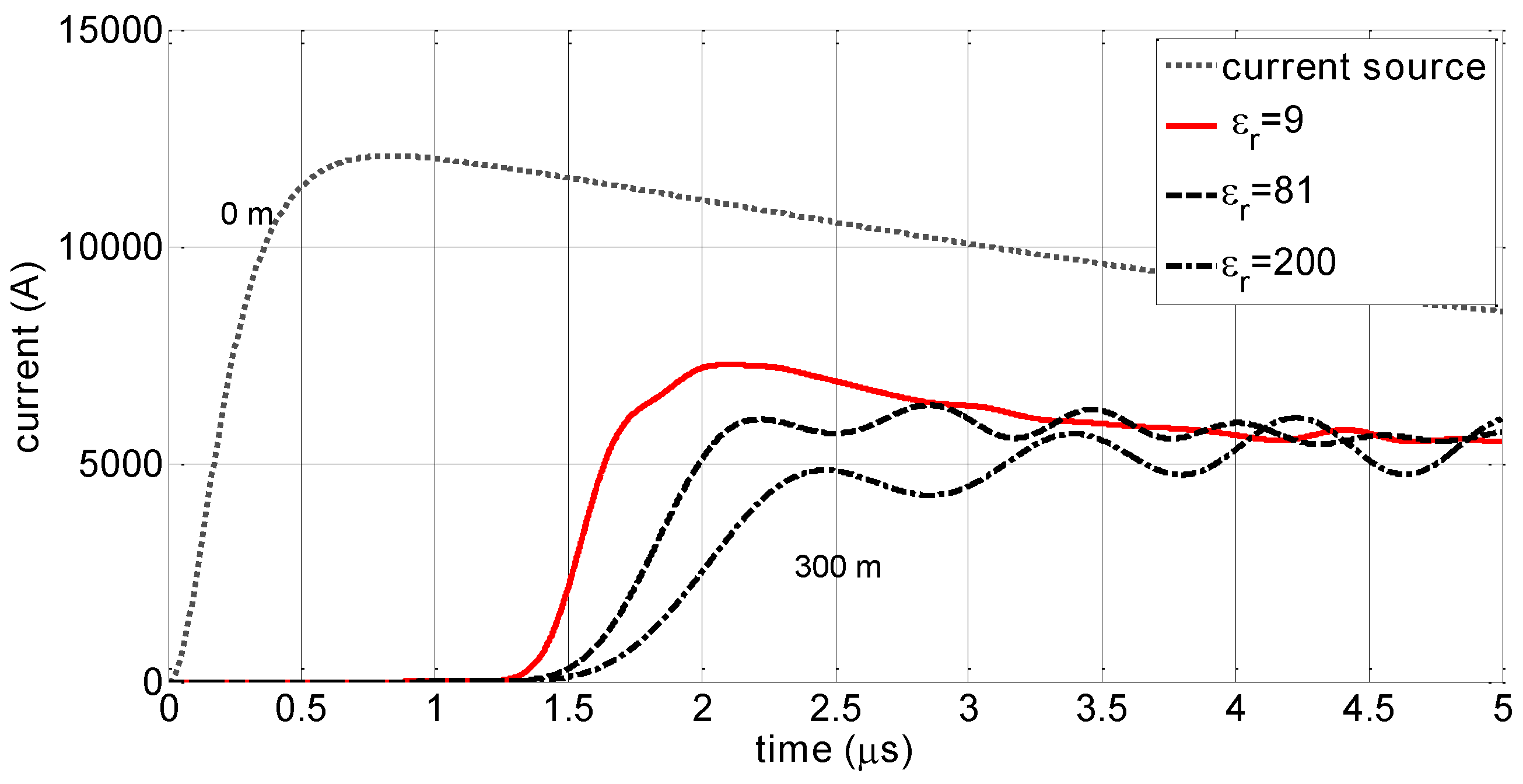
Figure 5 shows the current waveforms at the channel base and at a height of 300 m, considering 3 different values for the relative permittivity of the 4 × 4 m
2 parallelepiped dielectric, namely 9, 81 and 200. The resulting current speeds are about 0.71
c (for
εr = 9), 0.63
c (for
εr = 81), and 0.57
c (for
εr = 200). At the same time, increasing the relative permittivity results in an increase of the ripples on the current waveform.
It is also important to note that the size of the parallelepiped coating will also affect the current distribution along the channel as well as the resulting propagation speed. This is illustrated by the simulations presented in
Figure 6, where the current waveforms at the channel base and at a height of 300 m are evaluated varying the size of the coating (4 × 4, 6 × 6 and 8 × 8 m
2). As expected, it can be seen that increasing the size of the coating will result in higher dispersion of the current as well as a slower propagation speed.
Table 2 shows the computational time and memory resources needed to simulate a lightning channel embedded in a 2
d × 2
d m
2 parallelepiped dielectric coating with
εr = 1 and
μr = 1. It is clear that increasing either the relative permittivity of the dielectric or its thickness leads to an increase in the number of mesh cells and computational time and memory requirements.
Figure 7 shows the effect of the relative permeability of the coating on the current distribution, considering two cases. In the first case (
εr = 3,
μr = 3,
σ = 0 S/m), the resulting current wave propagation speed is about 0.64
c, a much lower value compared to that obtained for
εr = 9,
μr = 1, and
σ = 0.00 S/m. In the second case (
εr = 9,
μr = 9,
σ = 0.0005 S/m), the current wave propagation speed is slowed down to about 0.42
c. These results show that considering both permittivity and permeability of the coating as adjustable parameters allows better control of the desired return stroke propagation speed.
Table 3 shows the computational time and memory resources needed to simulate the lightning channel embedded in a 4 × 4 m
2 parallelepiped dielectric coating with given
εr and
μr. It is clear that increasing either the relative permittivity of the dielectric or its thickness leads to an increase in the number of mesh cells and computational time and memory resources.
2.3. A Wire in Free-Space Loaded by Distributed Series Inductance (Model C)
In this case, the electromagnetic return stroke channel is modeled as a thin wire surrounded by air (d = 0 or εr = 1, μr = 1) loaded by distributed series resistance (R) and/or inductance (L).
As for the previous models, in CST-MWS simulations the flat ground is modeled by a 10 × 10 m2 PEC plate located in the x-y plane. A 10-m discrete port is used as a lumped current source between the ground plane and the lightning channel. The 2-km long return-stroke channel is modeled by cascading 200 lumped elements in CST-MWS. Each lumped element is formed by a series RL circuit. The computational domain in this simulation is truncated in the same way as in the previous models and the bottom plane is again assumed to be a PEC surface. The same two symmetry planes are used in this simulation as in the previous cases to reduce the computational time and memory resources.
Figure 8 shows the current distribution along the lightning channel at different heights calculated by CST-MWS for
L = 4 μH/m and
R = 1 Ω/m over the bottom 500 m of the channel, and
L = 4 μH/m and
R = 6 Ω/m or channel heights between 500 m and 2000 m. The resulting current wave propagation speed along the channel is about 0.47
c. As mentioned in the Introduction, a height-dependent distributed resistance allows the model to reproduce all the experimentally observed features of lightning electromagnetic fields [
9]. As can be seen from
Figure 8, the current distribution along the channel is affected by numerical fluctuations.
The effect of the value of the series inductance on the current distribution along the lightning channel is illustrated in
Figure 9. The height-dependent resistance is the same as in
Figure 8. It can be seen that the speed of the current pulse can be controlled easily by changing the value of the distributed series inductance. For the considered cases of
L = 2, 4 and 8 μH/m, the values for the speed of the current wave along the channel are about 0.62
c, 0.45
c, and 0.38
c, respectively.
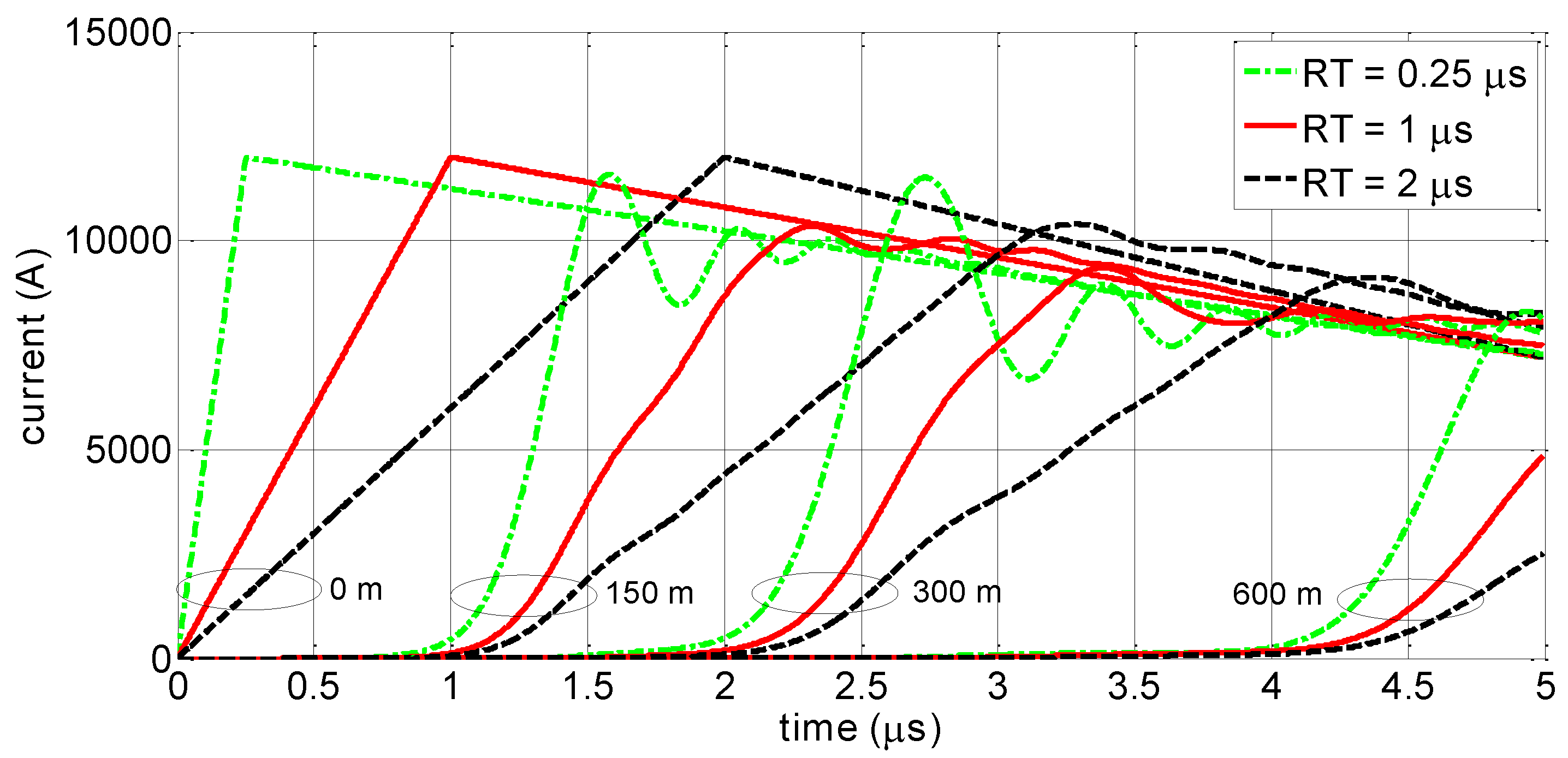
Finally,
Figure 10 illustrates the effect of the excitation current rise-time on the current distribution. In this case, a triangular waveshape with different risetimes (0.25, 1, and 2 microseconds) for the current is considered. Interestingly, the speed of the current wave along the channel appears to be nearly independent of the excitation risetime.
Table 4 shows the computational time and memory resources for this electromagnetic return-stroke model. In contrast with the other models, the variation of the adjustable parameters of this model does not affect either the memory resources or computational time.
3. Discussion
In this section, we present a discussion on the practical implementation of the considered electromagnetic models.
As mentioned in
Section 1, the main objective of the electromagnetic models proposed in the literature is to reproduce experimentally observed return stroke propagation speeds, which typically vary in the range of 1/3 to 2/3 the speed of light [
6,
16]. In this study, for each of the considered models, we determined the values for the adjustable parameters that allow obtaining the desired value of the return speed. Five typical values were considered, namely, 1 × 10
8 m/s, 1.3 × 10
8 m/s, 1.5 × 10
8 m/s, 1.8 × 10
8 m/s, and 2 × 10
8 m/s. The results are presented in
Table 5. According to this table, using any of the available representations, it is possible to reproduce the desired return-stroke speed by adequately adjusting the parameters. In some cases, however, the required parameters (i.e., high value of permittivity in
Model B) may result in fluctuations superimposed on the current distribution, as illustrated in simulations presented in the previous section.
Regarding the numerical performance of the considered electromagnetic models, the following comments can be made by comparing
Table 1,
Table 2,
Table 3,
Table 4 and
Table 5:
- -
Model A (wire embedded in a fictitious half-space dielectric medium) appears to be an efficient model in terms of the computation time and memory requirements. It should be noted, however, that this representation requires additional efforts for the computation of electromagnetic fields. Indeed, once the current distribution is obtained, an additional simulation should be carried out in free space, imposing the previously obtained current distribution.
- -
Model B (wire in a fictitious dielectric coating) circumvents the two-step simulation runs required by Model A. However, more significant computation time and memory requirements are needed. It is well known that the presence of an inhomogeneous medium with a relative permittivity higher than 1 can result in an increased number of mesh cells.
- -
The second variant of Model B (dielectric and ferromagnetic coating) is more expensive in terms of computing resources compared to its first variant (dielectric coating). However, this model is numerically more stable because it does not necessitate the use of a high permittivity to reproduce the typically observed return stroke speeds. On the other hand, it requires adjusting 3 parameters (d, εr, μr) to obtain the desired speed.
- -
Model C (wire loaded by distributed inductance and resistance) appears to be very efficient in terms of computer resources. Unlike other models, the variation of the adjustable parameters of this model does not affect either the memory resources or computational time. Also, considering a uniformly distributed resistance along the channel, the value of the return-stroke speed can be straightforwardly controlled by adjusting the per-unit-length series inductance.
4. Conclusions
In electromagnetic models, the return-stroke channel is represented as an antenna excited at its base by either a voltage or a current source. To adjust the speed of the current pulse propagating up the channel to available optical observations (in the order of 1/3 to 1/2 the speed of light), different representations for the return stroke channel have been proposed in the literature, including different techniques used to artificially reduce the propagation speed of the current pulse down to the range of observed values.
In this paper, we presented an analysis of the available electromagnetic models in terms of their practical implementation. Criteria used for the analysis were the ease of implementation of the models, numerical accuracy and needed computer resources, as well as their ability to reproduce a desired value for the speed of the current pulse.
Using CST-MWS software which is based on the time-domain FIT, different electromagnetic models were analyzed, namely Model A, a wire embedded in a fictitious half-space dielectric medium (other than air); Model B, a wire embedded in a fictitious coating with permittivity εr and permeability μr; and Model C, a wire in free-space loaded by distributed series inductance and resistance.
It was shown that by adjusting the parameters of each model, it is possible to reproduce a desired value for the speed of the return stroke current pulse. For each of the considered models, we determined the values for the adjustable parameters that allow the desired value of the return speed to be obtained.
Model A is the least expensive in terms of computing resources. However, it requires two simulation runs to obtain the electromagnetic fields. Furthermore, increasing the value of the relative permittivity leads to an increase in memory resources and computational time. A variant of Model B which includes a fictitious dielectric/ferromagnetic coating was found to be more efficient to control the current speed along the channel than using only a dielectric coating. On the other hand, this model requires an increased number of mesh cells, resulting in higher memory and computational time. The presence of an inhomogeneous medium generates unphysical fluctuations on the resulting current distributions. It has been shown that these fluctuations strongly depend on the size of the coating as well as on its electric and magnetic properties. In addition, it was shown that considering conductive losses in the coating would be an efficient way to attenuate these fluctuations.
Considering the efficiency in terms of the required computer resources and ease of implementation, we recommend the use of Model C (wire loaded by distributed inductance and resistance). In addition, among the considered models, Model C is the only one for which the memory resources and computational time are not affected by the variation of the adjustable parameters.
For each model, we derived the values for all the adjustable parameters to reproduce typically observed return-stroke wavefront speeds. These parameters are summarized in
Table 5 of the paper.
Note that we used the FIT technique implemented in CST for the presented analysis. Even though it is the first time FIT has been applied to electromagnetic models and it presents some advantages with respect to other, more popular models, the conclusions of the paper are, for the most part, applicable to other time domain solvers such as FDTD.
A final comment is in order on the use of full-wave numerical codes to implement electromagnetic models. As already mentioned, the electromagnetic models have received increased attention in recent years partly because of wider availability of full-wave numerical codes and increased computer capabilities. These full-wave numerical codes allow the simultaneous computation of the current distribution along the channel, the generated electromagnetic fields and the induced disturbances on nearby power systems or objects. Their application to lightning requires the use of artificial techniques to control the speed of the propagation of current pulse. As illustrated in this work, these artificial techniques can have various weaknesses such as the lack of physical justification or related numerical issues. It would therefore be desirable to work towards the development of more physically oriented models using the environment offered by today’s available full-wave codes.


