1. Introduction
Polycyclic Aromatic Hydrocarbons (PAHs), which are the byproduct of combustion, exist in the atmosphere in both gas and particulate phases. Naphthalene, which is the simplest PAH, consists of two fused benzene rings. Naphthalene and some of the other lower molecular weight PAHs can exist in the gas phase. However, most PAHs exist in the particulate phase, usually adsorbed onto the surface of fine particulate matter (i.e., particles with an aerodynamic diameter smaller than 2.5 μm).
Epidemiologic research over the last 30 years has shown increases in adverse cardiovascular and respiratory outcomes in relation to mass concentrations of particulate matter (PM) ≤2.5 μm or ≤10 μm in aerodynamic diameter (PM
2.5 and PM
10, respectively). A number of research papers [
1,
2,
3,
4,
5] have been published that examine the exposure and risk of Polycyclic Aromatic Hydrocarbons (PAHs) and their association with PM
2.5, PM
10 and ultrafine particles (UFPs). Many PAHs are known carcinogens [
6,
7,
8]. The US Environmental Protection Agency (EPA), whose role is to safeguard the population and the environment, has published both inhalation and oral chronic dose exposure estimates associated for PAHs [
9].
A relatively new area of focus in US EPA air quality research is measuring pollutants near roadways. It has been estimated that approximately 11% of households in the United States are located within 100 m of four-lane highways or expressways [
10]. In the past decade, studies have been conducted both nationally and internationally which focus on particles and gases that are emitted from mobile source exhaust from busy highways and freeways. The first major study [
11] was conducted in the United States in the Los Angeles Basin. Following the Los Angeles study, a number of researchers [
12,
13,
14,
15] have found that mobile sources on freeways can be a major source of fine and ultrafine PM and PAHs have been found in the fine and ultrafine particles fractions [
16,
17,
18].
The field study was conducted to: (1) yield 8-h integrated particle-bound PAH data from low flow particulate samplers located in close proximity (within 15 m) to a major roadway (Interstate 40); (2) compare the data against traffic data that was also collected at the monitoring station; (3) create wind roses from the wind vector data collected at the monitoring location and analyze the speciated PAHs against local sources; (4) compare the data against traffic data that was also collected at the monitoring station; and (5) compare and contrast the PAH data to photochemical oxidant measurements being analyzed at this monitoring site and draw associations and conclusions from that comparison.
2. Experiment
US EPA and the North Carolina Department of Environment and Natural Resources operate an air pollution monitoring station to meet the requirements for a fixed NO
2 near-road monitoring site.
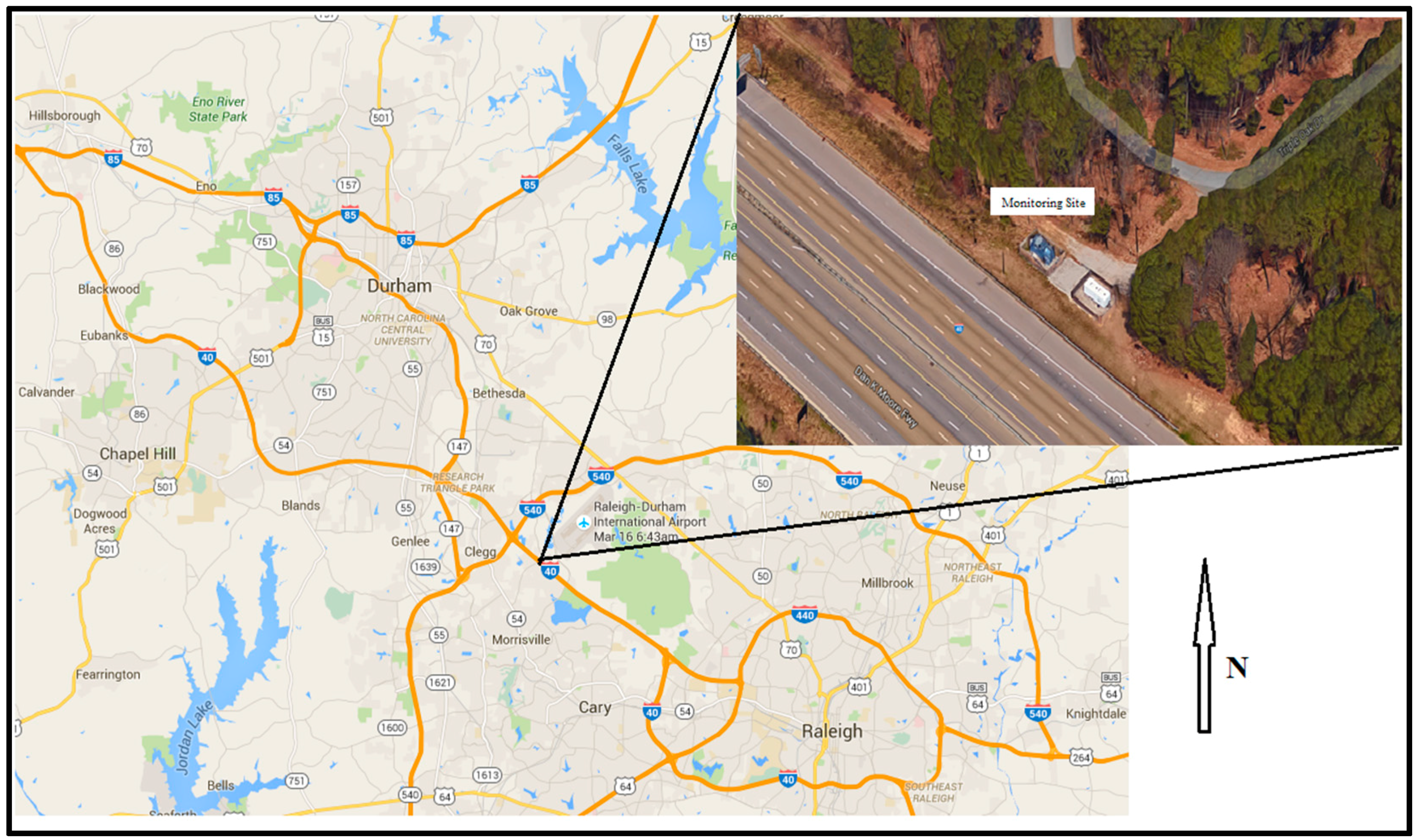
Figure 1 illustrates the location of the Research Triangle Park Near-Roadway station in relation to Raleigh, Durham and Chapel Hill, North Carolina. The inset shows the proximity of the station to the interstate. The fence of the monitoring stations is ~15 m from the edge of the roadway. The sampling occurred between 5 September and 6 November 2014, on a one-in-three day sampling schedule.
Table 1 illustrates the meteorological parameters during the study period. Please note that rainfall was intermittent during the sampling period with measurable rain occurring 7 of the 20 sampling days.
Sample collection was performed on 47 mm diameter Polytetrafluoroethylene (PTFE) filters. The filters were placed into low flow (~16.7 L/minute, BGI Incorporated model PQ200) discrete samplers with very sharp cut-point cyclones at aerodynamic size range of PM2.5. The samplers were mounted and operated along the freeway-facing fence inside the near roadway monitoring station. The inlets were positioned above the fenceline and had direct exposure to the interstate.
The sequential samplers were operated on three 8-h time slots. These were:
Sampler #1: 4 a.m.–12 p.m. (morning)
ampler #2: 12 p.m.–8 p.m. (afternoon)
Sampler #3: 8 p.m.–4 a.m., the next day. (nighttime)
The reasoning behind the staggered starting times was to capture the different “rush hour” commuting times between 6 and 10 a.m. and 4 and 8 p.m. on the highway. In addition, the sampling strategy allowed for the capture of the “nighttime” traffic when heavy duty diesel engines were expected to dominate the roadway. A total of 107 samples were collected. Of these 107 samples, 60 samples were collected using the 8-h samplers, seven field blanks were collected during the study and 40 samples were collected (i.e., two additional samplers) that were operated for 24 h. The 24 h samplers were considered to be the quality assurance samplers, which operated at the same time as the three 8-h samplers, i.e., 4 a.m. of one day to 4 a.m. of the next day.
In a temperature and humidity controlled laboratory, each sample filter was placed into a cassette and transported to the field using an aluminum cassette holder. The sample cassettes were loaded into the samplers and the time/date were entered and recorded in a field notebook. After each sampling event, the samples were removed from the samplers and transported in a temperature controlled container to a laboratory facility on the EPA campus in Research Triangle Park, North Carolina, where they were removed from the filter cassettes, placed in petri dishes and stored in a refrigerator at ~5 °C. The samples were stored in the refrigerator until the end of the sampling period and transported to North Carolina State University Chemistry Laboratory in Raleigh, North Carolina for analytical analysis.
Prior to the analysis, National Institute of Standards and Technology (NIST) traceable standards were obtained for the compounds listed in
Table 2. Several researchers [
17,
18,
19,
20,
21] provided details on the GC-MS analyses. The analysis methods utilized by these researchers provided a starting point for the temperature profile used for the GC-MS analyses for this project. However, it should be noted that each GC-MS is different and modifications to these methods were made until the NIST traceable standards eluted independently and illustrated excellent peak height and shape. In preparation for the GC-MS analysis, the filters were removed from the petri dishes and placed into 20-mL extraction vials. To each vial, 15 mL of dichloromethane was added. Each filter remained in the capped vial for 48 h. The aliquot was reduced to 2 mLs using steam bath in a fume hood. After the GC-MS was tuned, 1 µL of each aliquot was injected into an Agilent 6890 Series GC System coupled with an Agilent 5973 Network Mass Selective detector equipped with a J&W Scientific/Agilent Technologies DB-5 GC column with a helium carrier gas flow rate of 1 mL/min. The MS scan range was 50–350 mass to charge ratio (
m/
z). All chromatograms obtained from the samples were analyzed and cross-referenced against two mass spectral libraries in order to identify the compounds in the sample.
3. Results
3.1. Analysis of PAHs versus Wind Wind Speed and Wind Direction Vectors
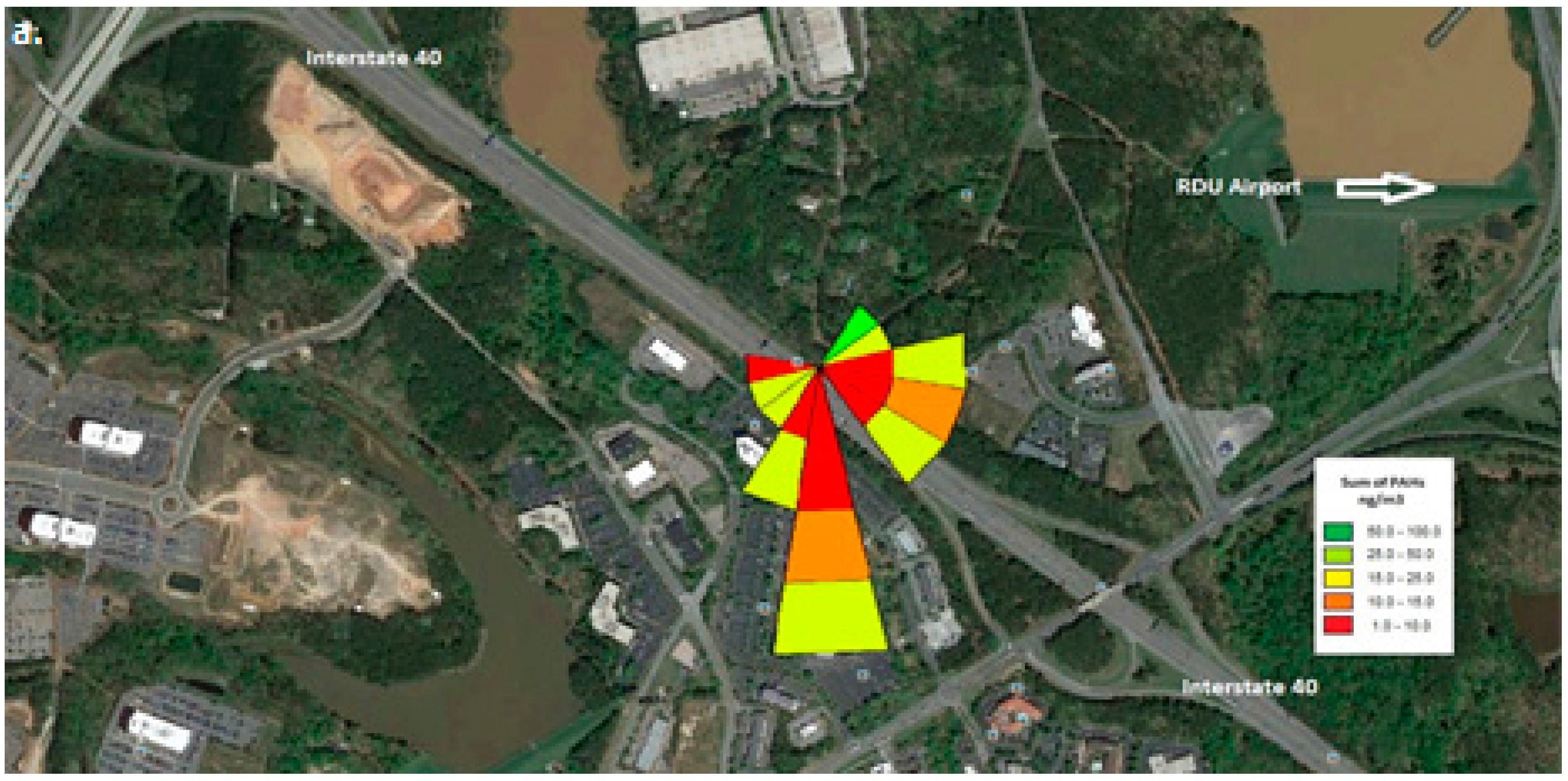
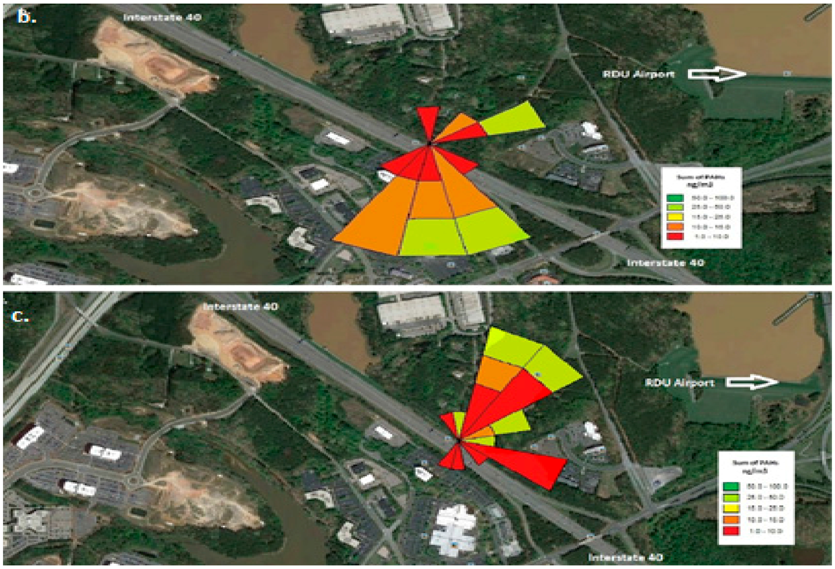
Wind roses were generated using the wind speed and wind direction vectors data that were collected at the monitoring location. As can be seen from
Figure 2, the interstate travels from northwest to southeast. The RDU international airport lies between northeast to east directions.
Figure 2 shows the pollutant rose for the three sampling time periods: morning, afternoon and nighttime.
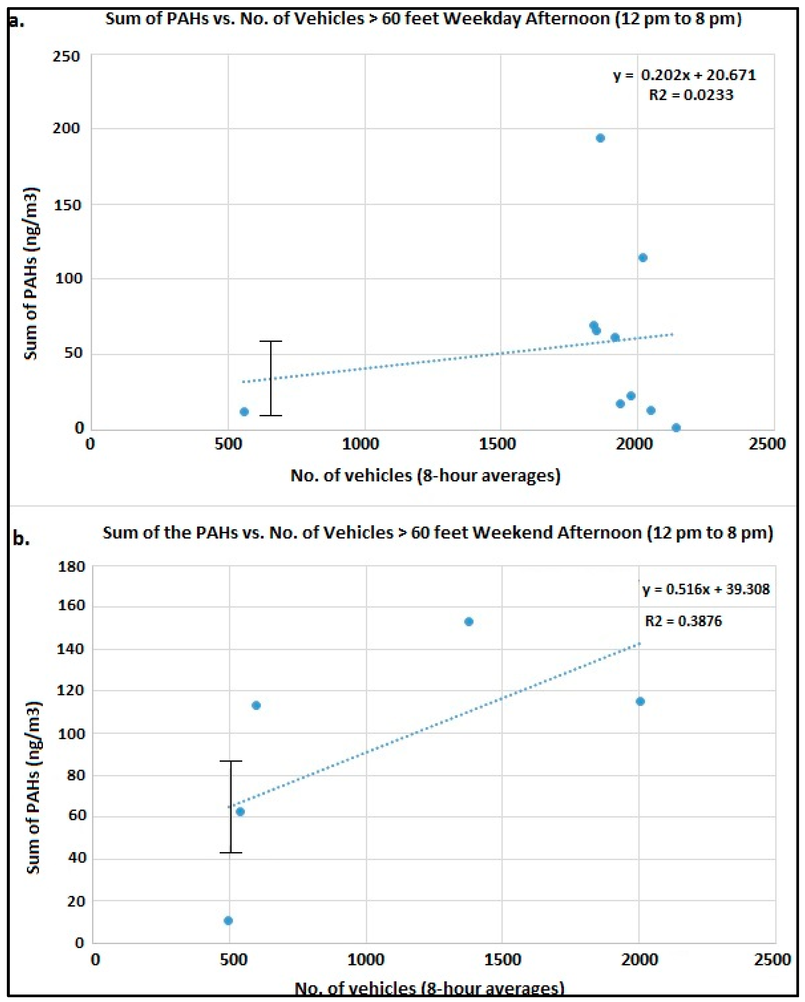
Figure 3a shows the trend plots of the sum of measured PAHs vs. Number of vehicles >60 feet in length (i.e., heavy duty diesel engine vehicles) during the afternoon (12 to 8:00 p.m.) on weekdays;
Figure 3b shows the number of vehicles >60 feet in length during the afternoon on weekends. We can conclude that when the wind direction is from the interstate to the measurement site i.e., afternoon there is a positive correlation with traffic (>60 feet) intensity. Similarly, during the night the airport and the traffic interchanges around it are the major contributors to the nighttime PAHs.
3.2. Analysis of Traffic Patterns
The overall average daily traffic (ADT) on the 20 sample days is ~146,000 vehicles per day. The average speed of the vehicles on these days was ~70 miles per hour. The distribution of the vehicles is skewed heavily toward vehicles that are 10–30 feet in length. The next largest group (during the morning and nighttime periods) are the vehicles that are greater than 60 feet in length (diesel engine vehicles). The second largest group in the afternoon period was the vehicles in the <10 feet in length.
Table 3 illustrates the distribution of the vehicles in the 6 different size categories.
As can be seen from
Table 3, ~90% of all vehicles are between 10 and 30 feet in length. The afternoon period, between 12 and 8 p.m. has the highest number of vehicles. The vehicles between 10 and 30 feet dominate during all three periods: 89.6%, 89.7% and 89.6%. There are some deviations in the other vehicles classes; the most significant deviation is during the nighttime period for the vehicles >60 feet in length. These vehicles account for 2%–3% of the morning and afternoon traffic, but make up 5.6% when measured against the total for the nighttime traffic.
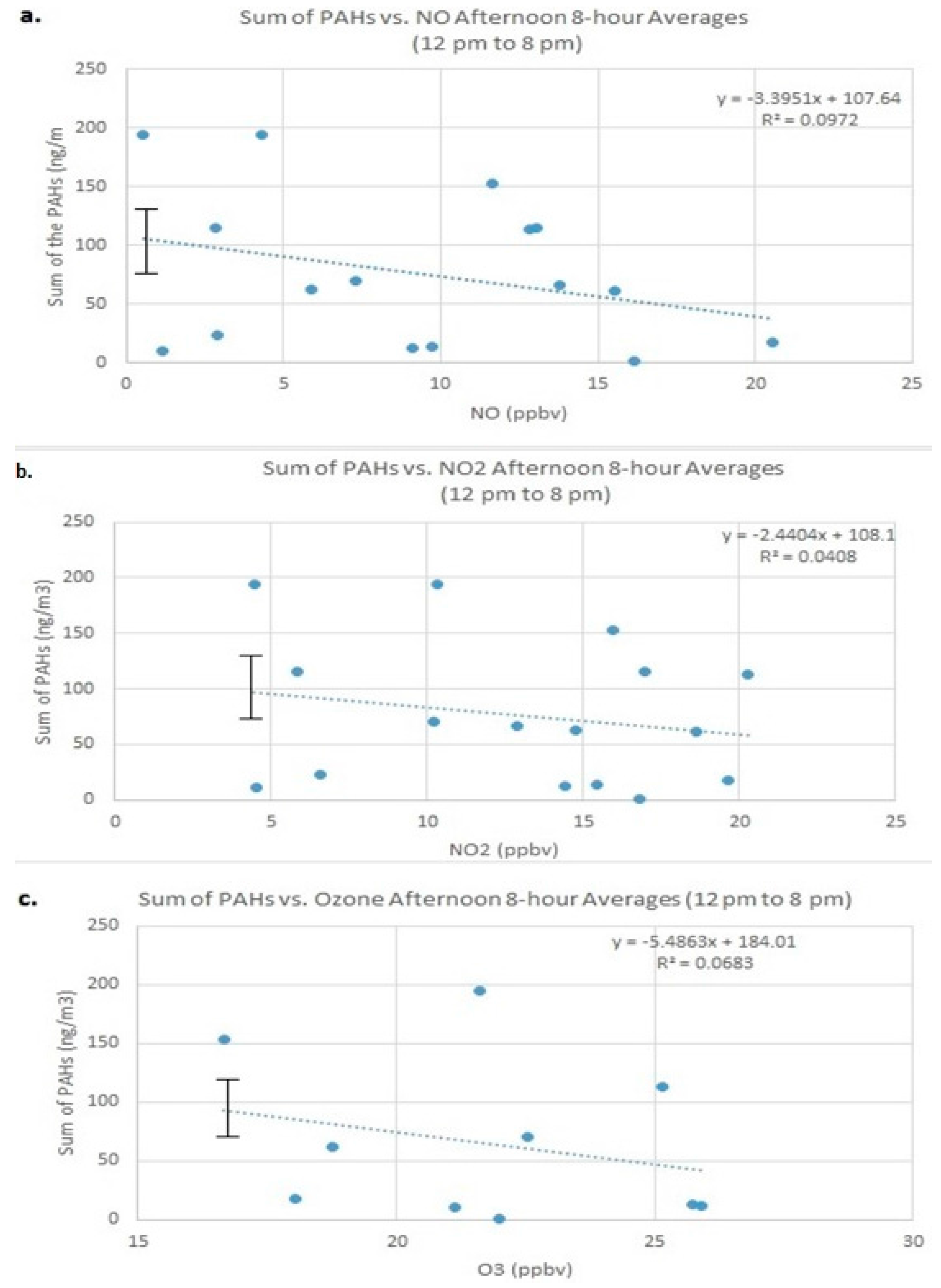
3.3. Analysis of PAHs versus Pollutant Data
Figure 4 illustrates the sum of the measured PAHs versus the afternoon (12 to 8 p.m.) photochemically active pollutants, NO, NO
2 and O
3. This time window provides the best estimate of the results of photochemical activity. Research suggests [
22,
23,
24,
25,
26,
27] that PAHs can react with NO, NO
2 and O
3. By examining
Figure 4, correlations can be observed between the sum of the PAHs with NO, NO
2 and O
3. A linear relationship can be seen between the PAHs and the pollutant data. Although there are correlations (R
2) between the NO, NO
2 and O
3 and sum of the measured PAHs (0.1, 0.04 and 0.07, respectively) there is discernable downward trend to the three graphs: as the pollutant concentrations increase, the sum of the PAHs decreases. In order to determine whether there is a significant relationship between the sum of the PAHs and the pollutant gases, an ANOVA regression was performed on the sum of the measured PAHs versus the three photochemical oxidants for the afternoon time period. With the alpha set at 5% (α = 0.05), the
p-values were calculated for the three gas pollutants against the sum of the measured PAHs. For an ANOVA statistical analysis, if the
p-value that is returned is less than 0.05, then the relationship between the two data sets is considered significant. The
p-value are 0.000264, 0.000496, and 0.00613, for NO, NO
2 and, O
3 respectively, which are all less than 0.05. These findings suggest that there is a weak, yet significant relationship between these two oxides of nitrogen species and ozone and that as the gas concentrations in the atmosphere increase, the overall concentration of the PAHs decrease, suggesting that these pollutant gases are interacting with PAHs and that the PAHs in the atmosphere are being chemically removed.
4. Discussion
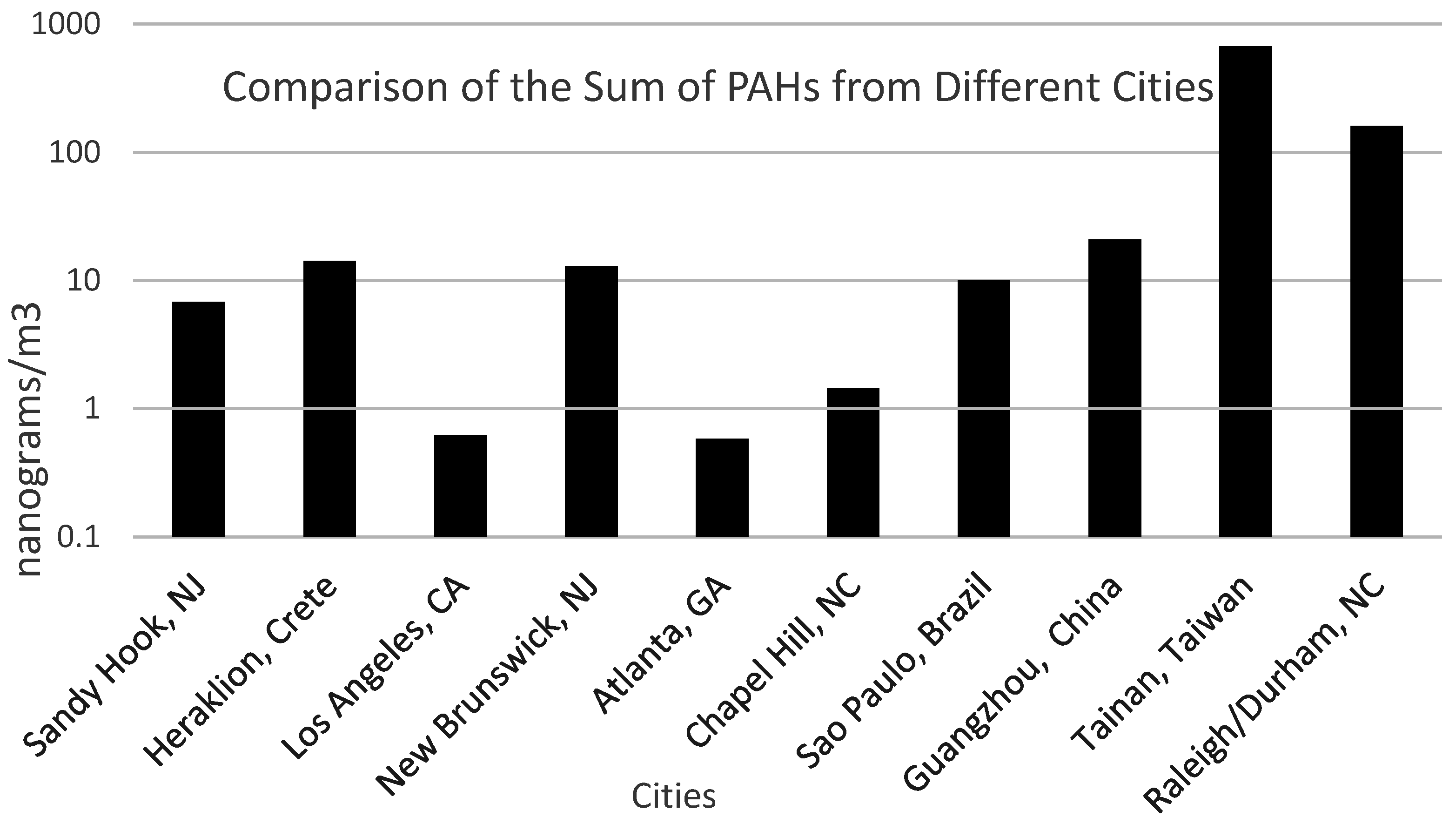
Figure 5 illustrates the results of this study compared to other published studies. Data from this research study compared well with data from other research studies [
28,
29,
30,
31,
32,
33,
34]. The sum of the concentrations of PAHs in rural, suburban and urban locations ranges between 0.5 and 20 ng/m
3. The sum of the PAH concentrations from this study was 160 ng/m
3. A similar research study [
34] performed at a busy intersection in Tainan, Taiwan, showed very high sum of the PAHs, ~667 ng/m
3.
5. Conclusions
This study provides a convenient methodology for collecting, extracting and analyzing for particle bound PAHs in three 8-h periods (morning, afternoon and nighttime) within a 24-h period. The results (0.1–21.6 nanogram/cubic meter ±9.0 std) agree with the published research literature (0.1 to 193.6 ng/m3) both nationally and internationally. There is a weak yet significant correlation between the PAHs with atmospheric oxidants. The distribution of the PAHs varied in relationship to the time of day. For afternoon hours, the PAH sources point to the interstate automobile emissions.
The published research studies focused on collection, analysis and interpretation of samples that were collected for 24-h periods or longer. Some rural studies collected samples over several days in order to collect enough sample for analysis. This study illustrated that if the sampling is close to the source, PAHs can be collected in 8-h segments using low flow (~16.7 lpm) PM2.5 samplers and source apportionment can be determined if meteorological data are available in the area.
Acknowledgments
The authors would like to thank Yang Zhang, North Carolina State University, Marine, Earth, and Atmospheric Sciences (MEAS); John Walker, EPA-Office of Research and Development (ORD), Research Triangle Park, North Carolina; Walter Robinson, Dept. Head North Carolina State University, MEAS; Sue Kimbrough, EPA-ORD, Richard Snow, EPA-ORD, Morteza Khaledi, Dept. Head North Carolina State University, Chemistry Department, Danielle Lehman, North Carolina State University, Chemistry Department Mass Spectrometry Lab. Dennis Mikel also would like to thank the EPA-ORD for providing access to the near-roadway station and use of the PM2.5 samplers during this study.
Author Contributions
Dennis K. Mikel conceived, designed and performed the experiment, analyzed the data and contributed reagents/materials/data analysis tools as part of his MS research. Dennis K. Mikel and Viney P. Aneja wrote the paper.
Conflicts of Interest
The authors declare no conflict of interest. The funding sponsors had no role in the design of the study; in the collection, analyses, or interpretation of data; in the writing of the manuscript, and in the decision to publish the results.
Abbreviations
The following abbreviations are used in this manuscript:
| PAHs | Polycyclic Aromatic Hydrocarbons |
| PM2.5 | Particulate Matter ≥2.5 microns in aerodynamic diameter |
| PM10 | Particulate Matter ≥10 microns in aerodynamic diameter |
| ANOVA | Analysis of Variance |
| UFP | Ultrafine Particulate |
| EPA | United States Environmental Protection Agency |
| NO | Nitric Oxide |
| NO2 | Nitrogen Dioxide |
| O3 | Ozone |
| GC-MS | Gas Chromatography-Mass Spectrometry |
| NIST | National Institute of Standards and Technology |
| ADT | Average Daily Traffic |
| R2 | R-squared, the correlation coefficient of a linear equation |
| ng/m3 | nanograms per cubic meter |
| RDU | Raleigh-Durham International Airport |
| μL | microliter |
| lpm | liters per minute |
| mL | milliliters |
| nm | nanometers |
References
- Vyskocil, A.; Fiala, Z.; Chenier, V.; Krajak, L.; Ettlerova, E.; Bukac, J.; Viau, C.; Emminger, S. Assessment of multipathway exposure of small children to PAH. Environ. Toxicol. Pharmacol. 2000, 8, 111–118. [Google Scholar] [CrossRef]
- Rajput, N.; Lakhani, A. PAHs and their carcinogenic potencies in diesel fuel and diesel generator exhaust. Hum. Ecol. Risk Assess. 2009, 15, 201–213. [Google Scholar] [CrossRef]
- Jyethi, D.S.; Khillare, P.; Sarkar, S. Risk assessment of inhalation exposure to polycyclic aromatic hydrocarbons in school children. Environ. Sci. Pollut. Res. 2014, 21, 366–378. [Google Scholar] [CrossRef] [PubMed]
- Seagrave, J.; Gigliotti, A.; McDonald, J.; Seilkop, S.; Whitney, K.; Zielinska, B.; Mauderly, J. Composition, toxicity, and mutagenicity of particulate and semivolatile emissions from heavy-duty compressed natural gas powered vehicles. Toxicol. Sci. 2005, 87, 232–241. [Google Scholar] [CrossRef] [PubMed]
- Fromme, H.; Oddoy, A.; Piloty, M.; Krause, M.; Lahrza, T. Polycyclic aromatic hydrocarbons PAH and diesel engine emission elemental carbon inside a car and a subway train. Sci. Total Environ. 1998, 217, 165–173. [Google Scholar] [CrossRef]
- Melendez-Colon, V.J.; Luch, A.; Seidel, A.; Baird, W. Cancer initiated by polycyclic aromatic hydrocarbons results from formation of stable DNA adducts rather than apurinic sites. Carcinogenesis 1999, 20, 1885–1891. [Google Scholar] [CrossRef] [PubMed]
- Bonner, M.; Han, D.; Nie, J.; Rogerson, P.; Vena, J.; Muti, P.; Freudenheim, J. Breast cancer risk and exposure in early life to polycyclic aromatic hydrocarbons using total suspended particulates as a proxy measure. Cancer Epidemiol. Biomark. Preview 2005, 14, 53–60. [Google Scholar]
- Nie, J.; Beyea, J.; Bonner, M.; Han, D.; Vena, J.; Rogerson, P.; Vito, D.; Muti, P.; Trevisan, M.; Edge, S.; et al. Exposure of traffic emissions throughout life and risk of breast cancer: The Western New York Exposures and Breast Cancer (WEB) study. Cancer Causes Control 2007, 18, 947–955. [Google Scholar] [CrossRef] [PubMed]
- Environmental Protection Agency. Risk Assessment for Carcinogens. Available online: http://www2.epa.gov/fera/risk-assessment-carcinogens (accessed on 15 January 2016).
- Brugge, D.; Durant, J.; Rioux, C. Near-highway pollutants in motor vehicle exhaust: A review of epidemiologic evidence of cardiac and pulmonary health risks. Environ. Health 2007, 6, 23–25. [Google Scholar] [CrossRef] [PubMed]
- Zhu, Y.; Hinds, W.; Kim, S.; Sioutas, C. Concentration and size distribution of ultrafine particles near a major highway. J. Air Waste Manag. Assoc. 2002, 9, 1032–1042. [Google Scholar] [CrossRef]
- Sioutas, C.; Delfino, R.; Singh, M. Exposure assessment for atmospheric ultrafine particles (UFPs) and Implications in epidemiologic research. Environ. Health Perspect. 2005, 113, 947–955. [Google Scholar] [CrossRef] [PubMed]
- Hagler, G.; Baldauf, R.; Thoma, E.; Long, T.; Snow, R.; Kinsey, J.; Oudejans, L.; Gullett, B. Ultrafine particles near a major roadway in Raleigh, North Carolina: Downwind attenuation and correlation with traffic-related pollutants. Atmos. Environ. 2009, 43, 1229–1234. [Google Scholar] [CrossRef]
- Kim, S.; Shen, S.; Sioutas, C.; Zhu, Y.; Hinds, W. Size distribution and diurnal and seasonal trends of ultrafine particles in source and receptor sites of the Los Angeles basin. J. Air Waste Manag. Assoc. 2002, 52, 297–307. [Google Scholar] [CrossRef] [PubMed]
- Shi, J.; Evans, D.; Khan, A.; Harrison, R. Sources and concentration of nanoparticles (10 nm diameter) in the urban atmosphere. Atmos. Environ. 2001, 35, 1193–1202. [Google Scholar] [CrossRef]
- Maciejczyk, P.B.; Offenberg, J.; Clemente, J.; Blaustein, M.; Thurston, G.; Chen, L. Ambient pollutant concentrations measured by a mobile laboratory in South Bronx, NY. Atmos. Environ. 2004, 38, 5283–5294. [Google Scholar] [CrossRef]
- Gigliotti, C.L.; Dachs, I.; Nelson, E.; Brunciak, P.; Eisenreich, S. Polycyclic aromatic hydrocarbons in the New Jersey Coastal Atmosphere. Environ. Sci. Technol. 2000, 34, 3547–3554. [Google Scholar] [CrossRef]
- Pleil, J.; Vette, A.; Rappaport, S. Assaying particle bound polycyclic aromatic hydrocarbons from archived PM2.5 filters. J. Chromatogr. 2003, 1033, 9–17. [Google Scholar] [CrossRef]
- Li, Z.; Sjodin, A.; Porter, E.; Patterson, D.; Needham, L.; Lee, S.; Russell, A.; Mulholland, J. Characterization of PM2.5-bound polycyclic aromatic hydrocarbons in Atlanta. Atmos. Environ. 2009, 43, 1043–1050. [Google Scholar] [CrossRef]
- Chen, S.-J.; Hwang, P.-S.; Hsieh, L.-T. The height variation and particle size distribution of polycyclic aromatic hydrocarbons in the ambient air. Toxicol. Environ. Chem. 1997, 60, 111–128. [Google Scholar] [CrossRef]
- Allen, A.G.; da Rocha, G.; Cardoso, A.; Machado, W.P.C.; de Andrade, J. Atmospheric particulate polycyclic aromatic hydrocarbons from road transport in southeast Brazil. Transp. Res. 2008, 13, 483–490. [Google Scholar] [CrossRef]
- Butler, J.; Crossley, P. Reactivity of Polycyclic Aromatic Hydrocarbons absorbed on soot particles. Atmos. Environ. 1980, 15, 91–94. [Google Scholar] [CrossRef]
- Feilberg, A.; Poulson, M.; Nielsen, T.; Skov, H. Occurrence and sources of particulate nitro-polycyclic aromatic hydrocarbons in ambient air in Denmark. Atmos. Environ. 2001, 35, 353–366. [Google Scholar] [CrossRef]
- Bamford, H.; Baker, J. Nitro-polycyclic aromatic hydrocarbon concentrations and sources in urban and suburban atmospheres of the mid-Atlantic region. Atmos. Environ. 2003, 37, 2077–2091. [Google Scholar] [CrossRef]
- Pitts, J.N.; van Cauwenberghe, K.; Grosjean, D.; Schmid, J.; Fitz, D.; Belser, W.; Knudson, G.; Hynds, P. Atmospheric reactions of polycyclic aromatic hydrocarbons: Facile formation of mutagenic nitro derivatives. Science 1978, 202, 515–519. [Google Scholar] [CrossRef] [PubMed]
- Nikolaou, K.; Masclet, P.; Mouvier, G. Sources and chemical reactivity of polynuclear aromatic hydrocarbons in the atmosphere—A critical review. Sci. Total Environ. 1984, 32, 103–132. [Google Scholar] [CrossRef]
- Kormacher, W.; Mamantov, G.; Wehry, E.; Natush, D. Resistance to photochemical decomposition of polycyclic aromatic hydrocarbons, vapor-adsorbed on coal fly ash. Environ. Sci. Technol. 1980, 14, 1094–1099. [Google Scholar] [CrossRef]
- Gao, B.; Yu, J.-Z.; Li, S.-X.; Ding, X.; He, Q.-F.; Wang, X.-M. Roadside and rooftop measurements of polycyclic aromatic hydrocarbons in PM2.5 in urban Guangzhou: Evaluation of vehicular and regional combustion source contributions. Atmos. Environ. 2011, 45, 7184–7191. [Google Scholar] [CrossRef]
- Bourotte, C.; Forti, M.; Taniguchi, S.; Bicego, M.; Lotufo, P. A wintertime study of PAHs in fine and coarse aerosols in Sao Paulo city, Brazil. Atmos. Environ. 2005, 39, 3799–3811. [Google Scholar] [CrossRef]
- Li, J.; Zhang, G.; Li, X.; Qi, S.; Liu, G.; Peng, X. Source seasonality of polycyclic aromatic hydrocarbons (PAHs) in a subtropical city, Guangzhou, South China. Sci. Total Environ. 2006, 355, 145–155. [Google Scholar] [CrossRef] [PubMed]
- Eiguren-Fernandez, A.; Miguel, A.; Froines, J.; Thurairatnam, S.; Avol, E. Seasonal and spatial variation of polycyclic aromatic hydrocarbons in vapor-phase and PM2.5 in Southern California urban and rural communities. Aerosol Sci. Technol. 2004, 38, 447–455. [Google Scholar] [CrossRef]
- Tsapakis, M.; Stephanou, E. Polycyclic aromatic hydrocarbons in the atmosphere of the Eastern Mediterranean. Environ. Sci. Technol. 2005, 39, 6584–6590. [Google Scholar] [CrossRef] [PubMed]
- Tsapakis, M.; Stephanou, E. Occurrence of gaseous and particulate poly-cyclic aromatic hydrocarbons in the urban atmosphere: Study of sources and ambient temperature effect on the gas/particle concentration and distribution. Environ. Pollut. 2005, 133, 147–156. [Google Scholar] [CrossRef] [PubMed]
- Shue, H.-L.; Lee, W.-J.; Lin, S.; Guor-Cheng, F.; Chang, H.-C.; You, W.-C. Particle-bound PAH content in ambient air. Environ. Pollut. 1997, 96, 369–382. [Google Scholar] [CrossRef]
© 2016 by the authors; licensee MDPI, Basel, Switzerland. This article is an open access article distributed under the terms and conditions of the Creative Commons Attribution (CC-BY) license (http://creativecommons.org/licenses/by/4.0/).


