
Mass Deposition Fluxes of Asian Dust to the Bohai Sea and Yellow Sea from Geostationary Satellite MTSAT: A Case Study


Abstract
:1. Introduction
2. Data and Radiative Transfer Models
2.1. Multifunctional Transport Satellites 1R (MTSAT-1R) Observations

| Channel | Wavelength /μm | Quantization Levels/bit | Space Resolution/km |
|---|---|---|---|
| Visible (VIS) | 0.55–0.90 | 10 | 1 |
| Thermal IR 1 (IR1) | 10.3–11.3 | 10 | 4 |
| Thermal IR 2 (IR2) | 11.5–12.5 | 10 | 4 |
| IR water vapor (IR3) | 6.5–7.0 | 10 | 4 |
| Mid-IR (R4) | 3.5–4.0 | 10 | 4 |
2.2. Streamer
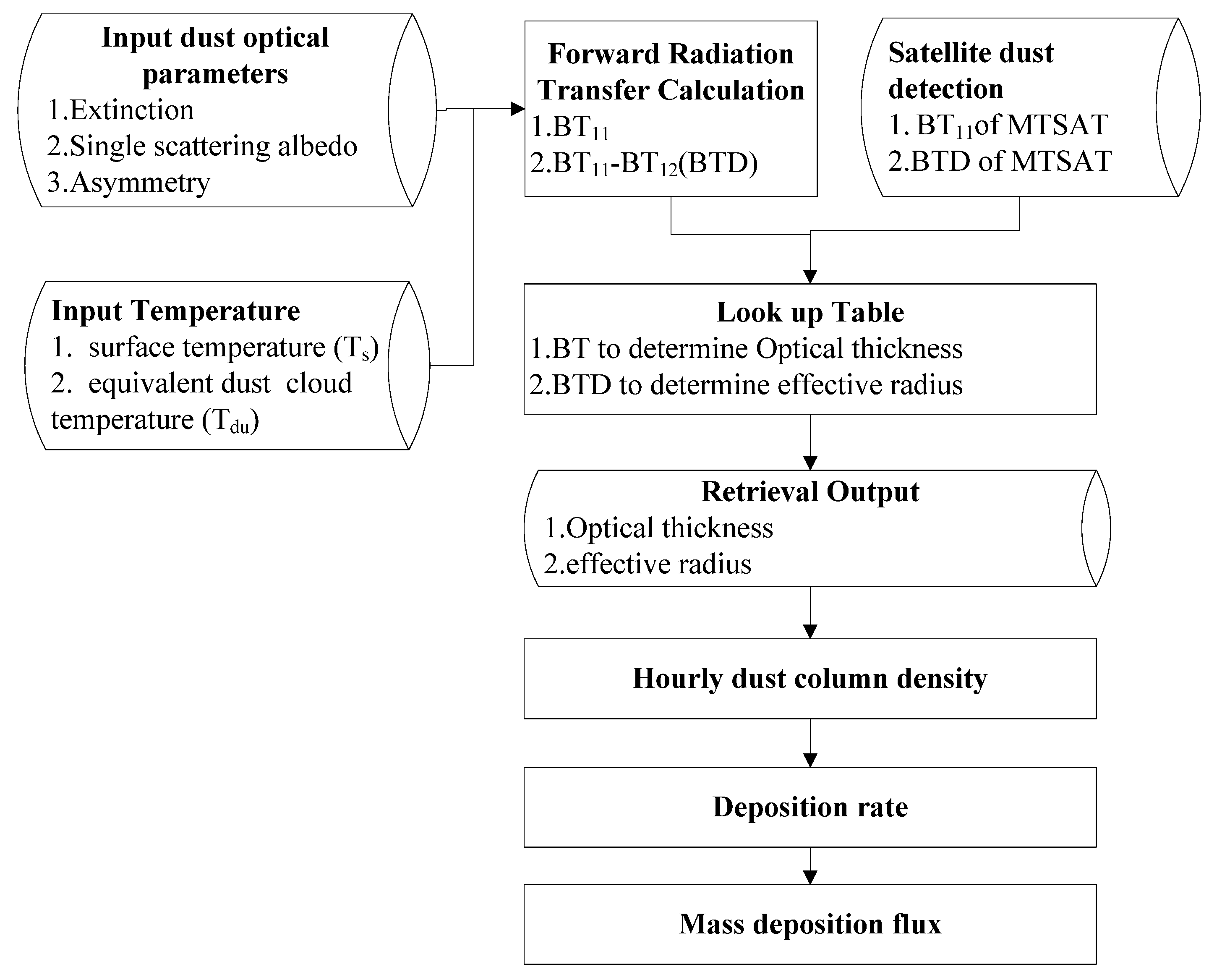
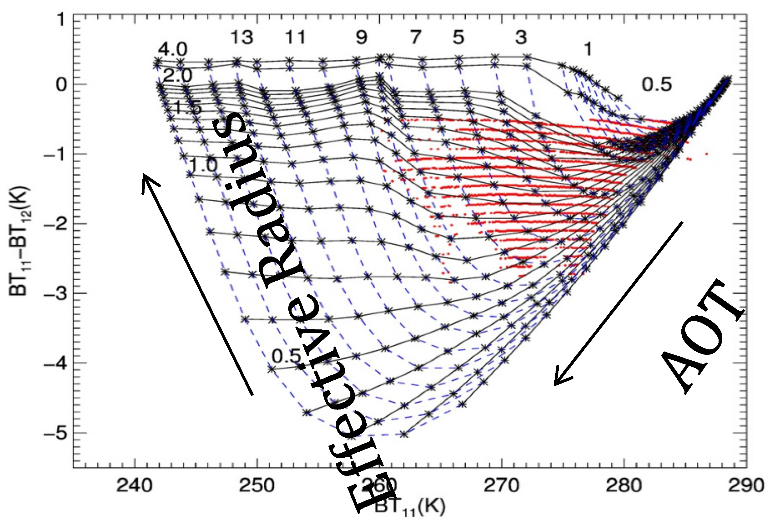
3. Methodology

| Parameter | Value |
|---|---|
| Atmospheric profiles | User-defined by radiosonde data |
| surface type | water |
| emissivity | 0.98 |
| Surface temperatures (K) | (265~295 (5)),bracketed text indicates step |
| dust temperatures (K) | (260~290 (5)), bracketed text indicates step |
| dust cloud bottom height (km) | 0.5 |
| optical thickness | (0.3~1.0 (0.1), 1.0~15.0 (1)) |
| effective radius (μm) | (0.1~2.0 (0.1), 2~10 (1)) |
4. Study Case
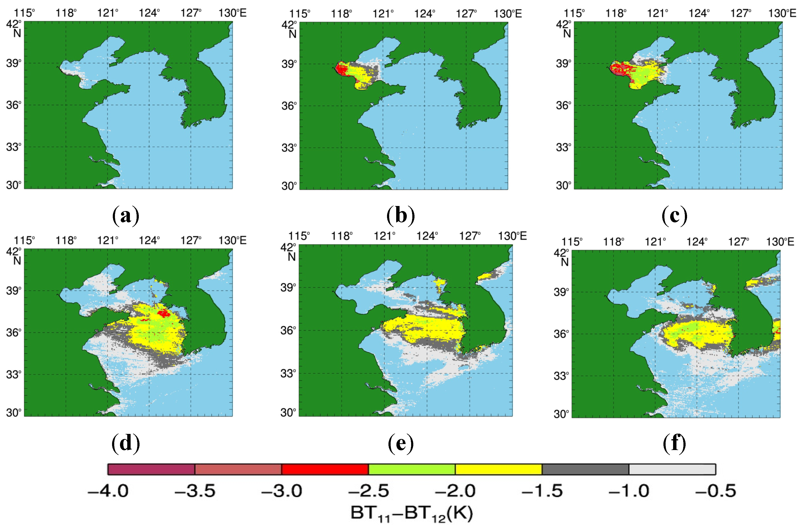
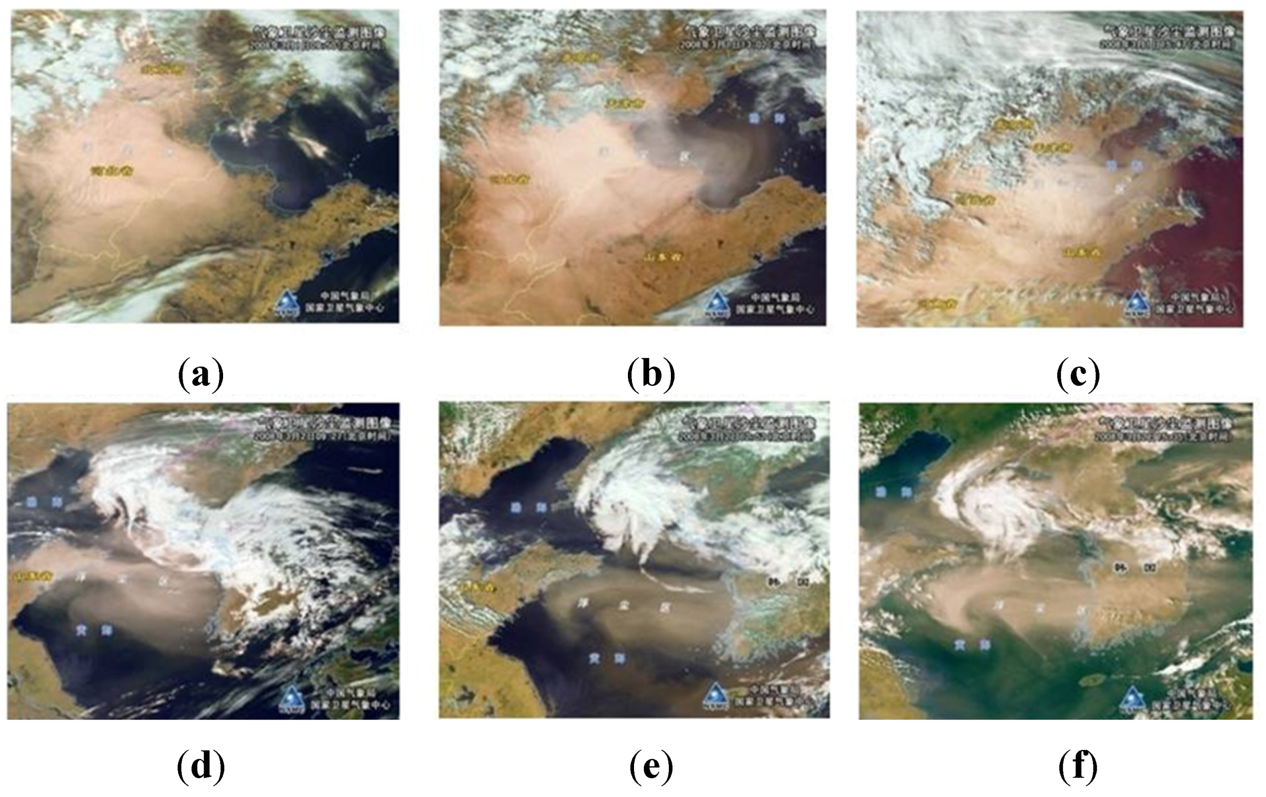
4.1. Dust Detection

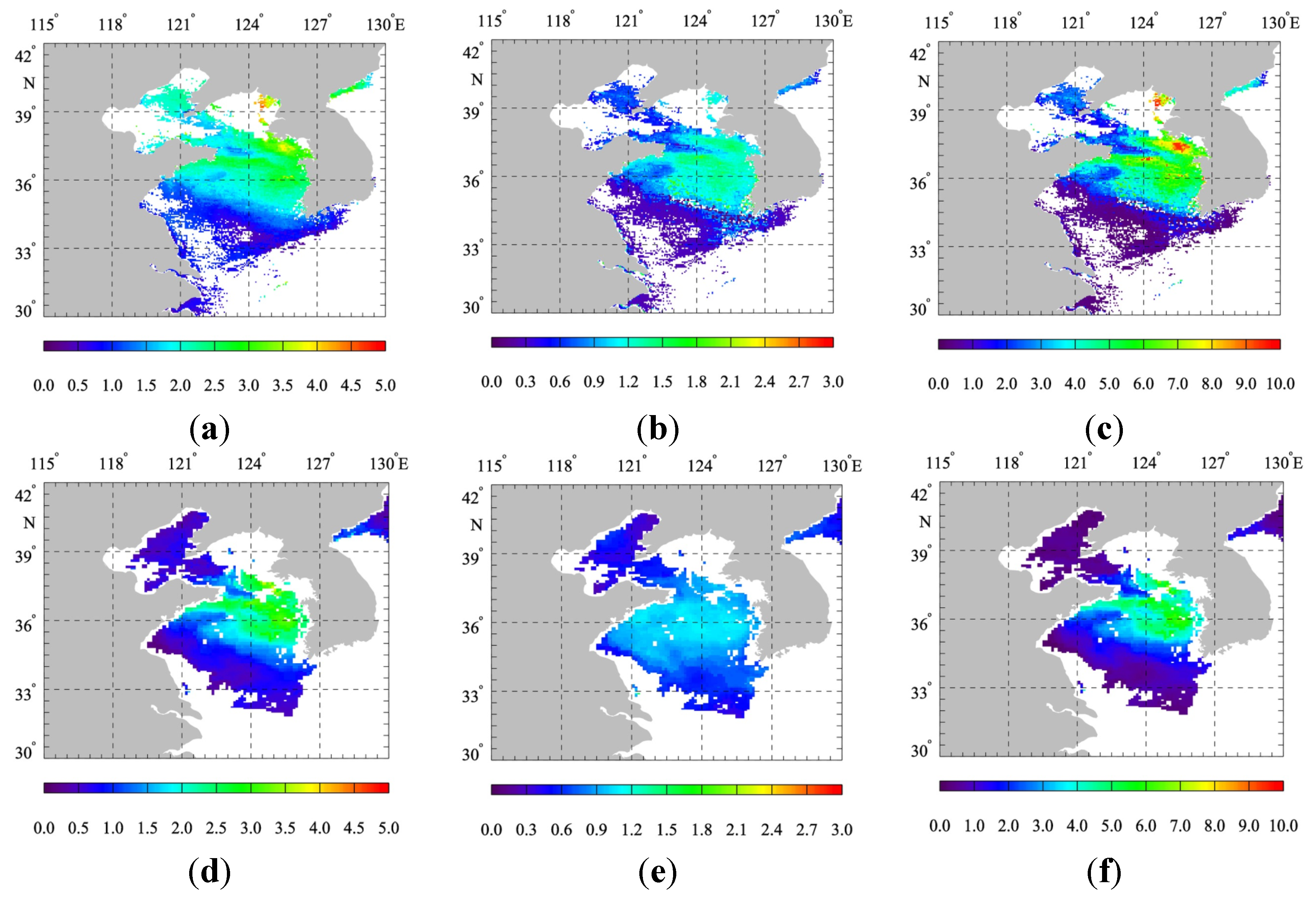
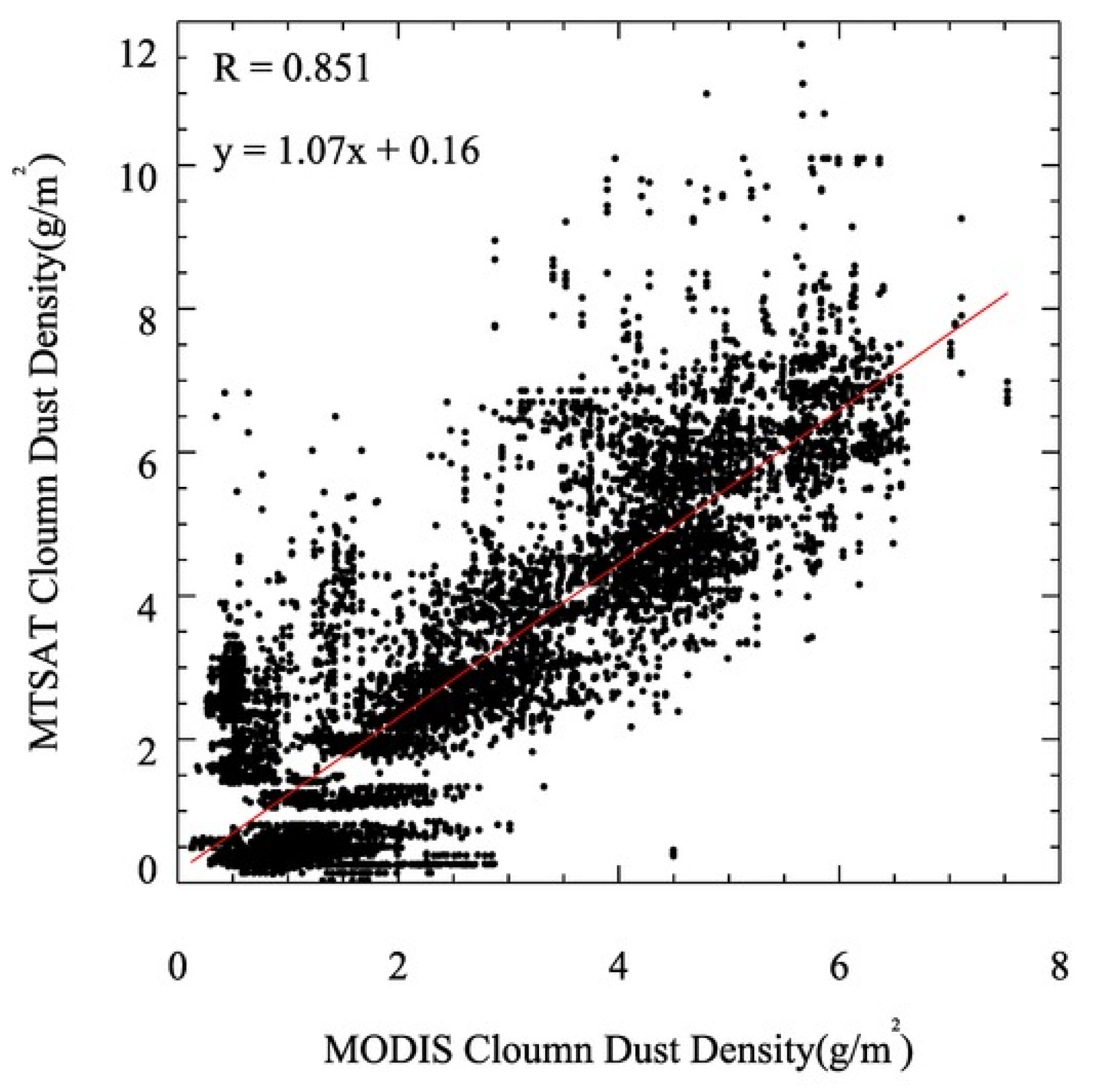
4.2. MTSAT-Derived Dust Properties Mapping and Comparison


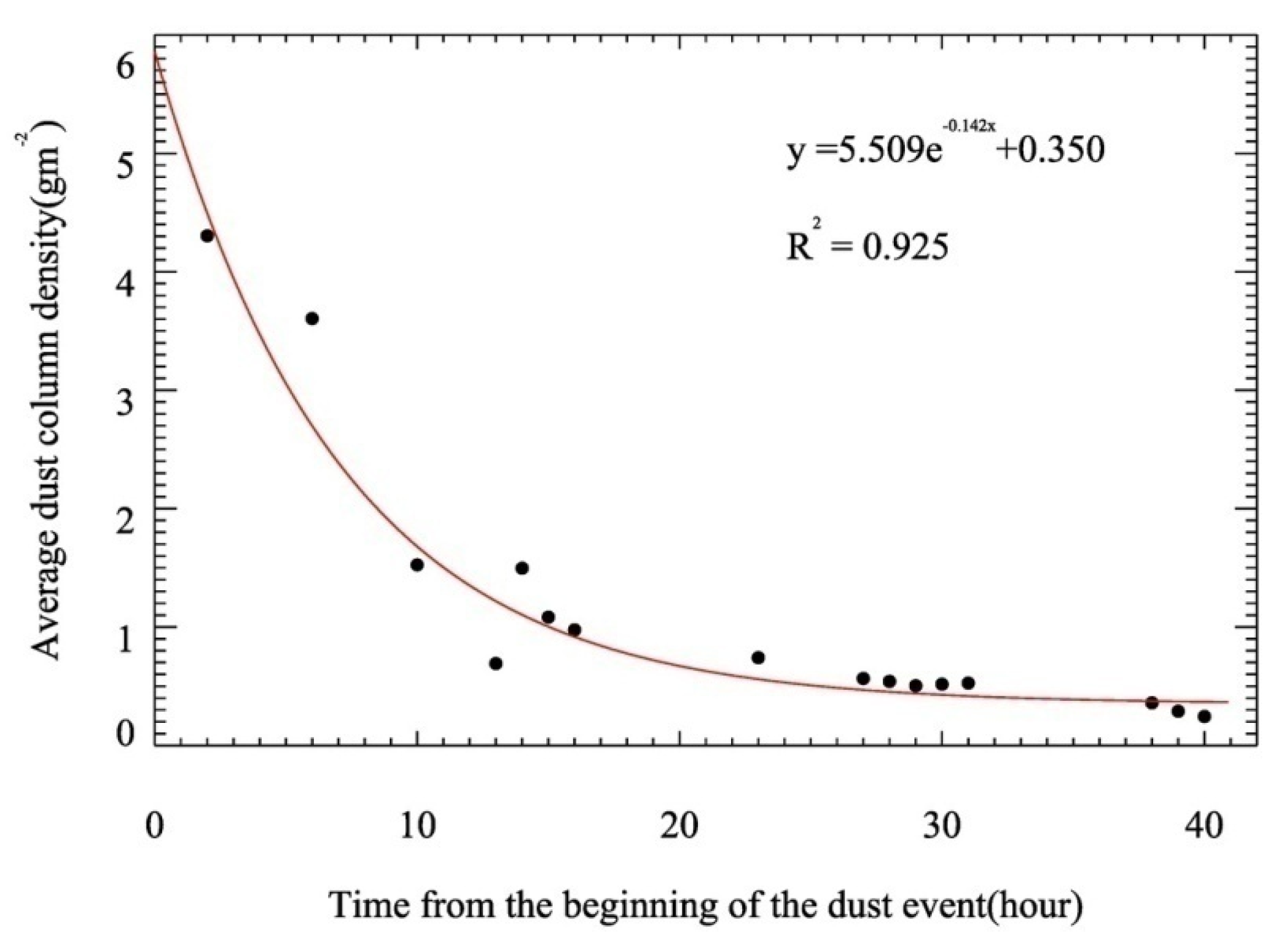
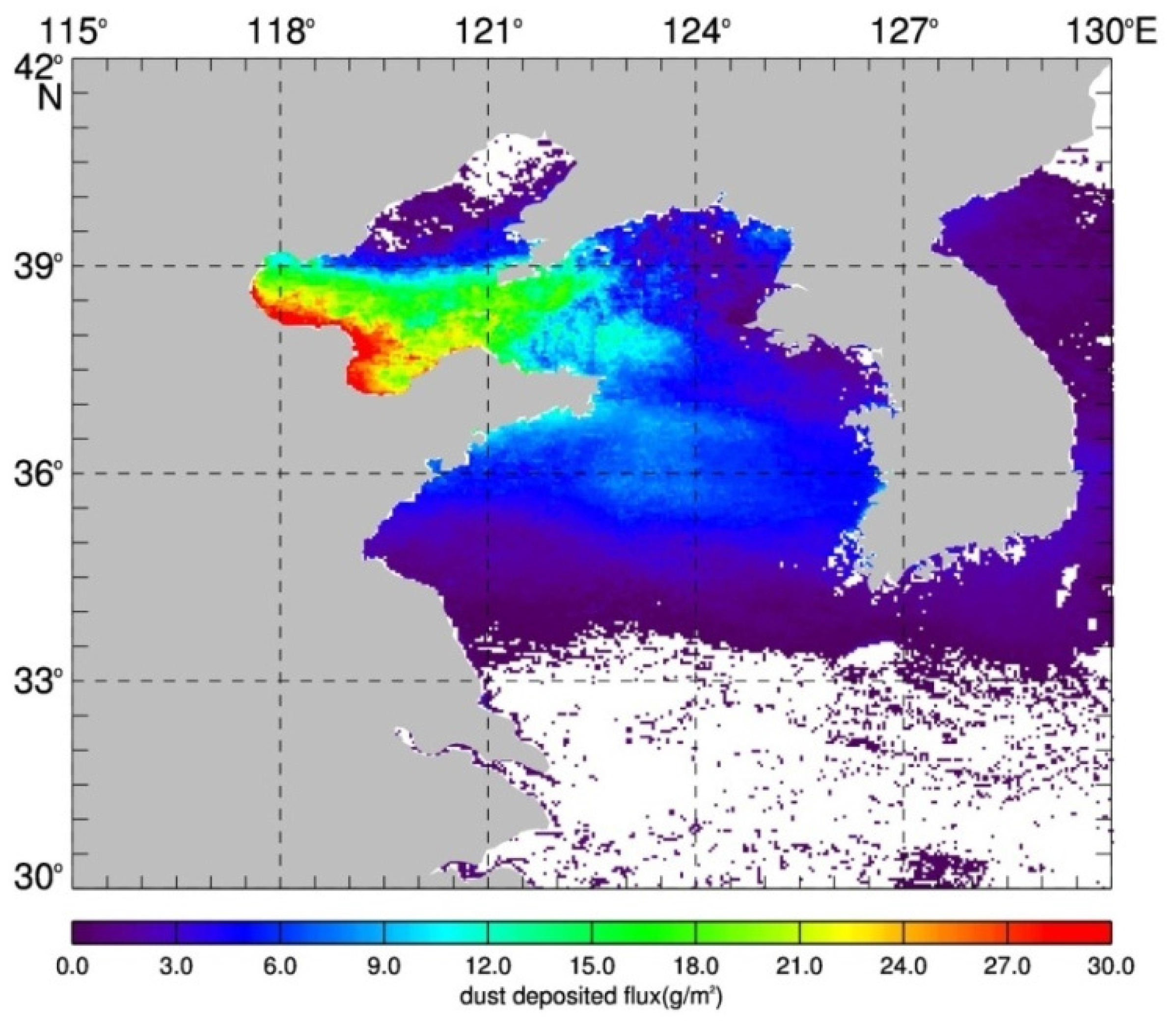
4.3. Estimation of the Total Deposited Mass


| Authors | Time Period | Methods | The Bohai Sea | The Yellow Sea |
|---|---|---|---|---|
| Liu and Zhou [28] | 1987–1992 | cruise track | 26.4 | 9.3 |
| Uematsu et al. [29] | 1994–1995 | model | 17.5 | 9.7 |
| Gao et al. [30] | 1989 | sites | 30~196 | 8.6~79 |
5. Conclusions
Acknowledgments
Author Contributions
Conflicts of Interest
References
- Mikami, M.; Shi, G.Y.; Uno, I.; Yabuki, S.; Iwasaka, Y.; Yasui, M.; Aoki, T.; Tanaka, T.Y.; Kurosaki, Y.; Masuda, K.; et al. Aeolian dust experiment on climate impact: An overview of japan-china joint project adec. Global Planet. Change 2006, 52, 142–172. [Google Scholar] [CrossRef]
- Sokolik, I.N.; Winker, D.M.; Bergametti, G.; Gillette, D.A.; Carmichael, G.; Kaufman, Y.J.; Gomes, L.; Schuetz, L.; Penner, J.E. Introduction to special section: Outstanding problems in quantifying the radiative impacts of mineral dust. J. Geophys. Res. -Atmos. 2001, 106, 18015–18027. [Google Scholar] [CrossRef]
- Tagliabue, A.; Aumont, O.; Bopp, L. The impact of different external sources of iron on the global carbon cycle. Geophys. Res. Lett. 2014, 41, 920–926. [Google Scholar] [CrossRef]
- Jickells, T.D.; An, Z.S.; Andersen, K.K.; Baker, A.R.; Bergametti, G.; Brooks, N.; Cao, J.J.; Boyd, P.W.; Duce, R.A.; Hunter, K.A.; et al. Global iron connections between desert dust, ocean biogeochemistry, and climate. Science 2005, 308, 67–71. [Google Scholar] [CrossRef] [PubMed]
- Mahowald, N.M.; Baker, A.R.; Bergametti, G.; Brooks, N.; Duce, R.A.; Jickells, T.D.; Kubilay, N.; Prospero, J.M.; Tegen, I. Atmospheric global dust cycle and iron inputs to the ocean. Global Biogeochem. Cycles 2005. [Google Scholar] [CrossRef]
- Shi, J.-H.; Zhang, J.; Gao, H.-W.; Tan, S.-C.; Yao, X.-H.; Ren, J.-L. Concentration, solubility and deposition flux of atmospheric particulate nutrients over the yellow sea. Deep-Sea Res. Part Ii-TopicalStud. in Oceanogr. 2013, 97, 43–50. [Google Scholar] [CrossRef]
- Tan, S.-C.; Wang, H. The transport and deposition of dust and its impact on phytoplankton growth in the yellow sea. Atmos. Environ. 2014, 99, 491–499. [Google Scholar] [CrossRef]
- Yuan, W.; Zhang, J. High correlations between asian dust events and biological productivity in the western north pacific. Geophys. Res. Lett. 2006. [Google Scholar] [CrossRef]
- Niedermeier, N.; Held, A.; Muller, T.; Heinold, B.; Schepanski, K.; Tegen, I.; Kandler, K.; Ebert, M.; Weinbruch, S.; Read, K.; et al. Mass deposition fluxes of saharan mineral dust to the tropical northeast atlantic ocean: An intercomparison of methods. Atmos. Chem. Phys. 2014, 14, 2245–2266. [Google Scholar] [CrossRef] [Green Version]
- Ginoux, P.; Chin, M.; Tegen, I.; Prospero, J.M.; Holben, B.; Dubovik, O.; Lin, S.J. Sources and distributions of dust aerosols simulated with the gocart model. J. Geophys. Res. -Atmos. 2001, 106, 20255–20273. [Google Scholar] [CrossRef]
- Zender, C.S.; Bian, H.S.; Newman, D. Mineral Dust Entrainment and Deposition (DEAD) model: Description and 1990s dust climatology. J. Geophys. Res. -Atmos. 2003. [Google Scholar] [CrossRef]
- Wang, Z.F.; Ueda, H.; Huang, M.Y. A deflation module for use in modeling long-range transport of yellow sand over east asia. J. Geophys. Res. -Atmos. 2000, 105, 26947–26959. [Google Scholar] [CrossRef]
- Uno, I.; Carmichael, G.R.; Streets, D.G.; Tang, Y.; Yienger, J.J.; Satake, S.; Wang, Z.; Woo, J.H.; Guttikunda, S.; Uematsu, M.; et al. Regional chemical weather forecasting system cfors: Model descriptions and analysis of surface observations at japanese island stations during the ace-asia experiment. J. Geophys. Res. -Atmos. 2003. [Google Scholar] [CrossRef]
- Huneeus, N.; Schulz, M.; Balkanski, Y.; Griesfeller, J.; Prospero, J.; Kinne, S.; Bauer, S.; Boucher, O.; Chin, M.; Dentener, F.; et al. Global dust model intercomparison in aerocom phase i. Atmos. Chem. Phys. 2011, 11, 7781–7816. [Google Scholar] [CrossRef] [Green Version]
- Wen, S.; Rose, W.I. Retrieval of sizes and total masses of particles in volcanic clouds using AVHRR bands 4 and 5. J. Geophys. Res. 1994, 99, 5421–5421. [Google Scholar] [CrossRef]
- Gu, Y.; Rose, W.I.; Bluth, G.J.S. Retrieval of mass and sizes of particles in sandstorms using two MODIS IR bands: A case study of April 7, 2001 sandstorm in China. Geophys. Res. Lett. 2003. [Google Scholar] [CrossRef]
- Tanre, D.; Kaufman, Y.J.; Herman, M.; Mattoo, S. Remote sensing of aerosol properties over oceans using the modis/eos spectral radiances. J. Geophys. Res. -Atmos. 1997, 102, 16971–16988. [Google Scholar] [CrossRef]
- Kaufman, Y.J.; Koren, I.; Remer, L.A.; Tanre, D.; Ginoux, P.; Fan, S. Dust transport and deposition observed from the terra-moderate resolution imaging spectroradiometer (MODIS) spacecraft over the atlantic ocean. J. Geophys. Res. -Atmos. 2005. [Google Scholar] [CrossRef]
- Zhang, P.; Lu, N.; Hu, X.; Dong, C. Identification and physical retrieval of dust storm using three modis thermal ir channels. Global Planet. Change 2006, 52, 197–206. [Google Scholar] [CrossRef]
- Sohn, B.J.; Park, H.S.; Han, H.J.; Ahn, M.H. Evaluating the calibration of MTSAT-1R infrared channels using collocated Terra MODIS measurements. Int. J. Remote Sens. 2008, 29, 3033–3042. [Google Scholar] [CrossRef]
- Key, J. Streamer User’s Guide; Cooperative Institute for Meteorological Satellite Studies, University of Wisconsin: Wisconsin, WI, USA, 2001. [Google Scholar]
- Stamnes, K.; Tsay, S.C.; Wiscombe, W.; Jayaweera, K. Numerically stable algorithm for discrete-ordinate-method radiative-transfer in multiple-scattering and emitting layered media. Appl. Opt. 1988, 27, 2502–2509. [Google Scholar] [CrossRef] [PubMed]
- Zhang, P.; Lu, N.; Hu, X.; Dong, C. Identification and physical retrieval of dust storm using three modis thermal ir channels. Global Planet. Change 2006, 52, 197–206. [Google Scholar] [CrossRef]
- Hao, Z.; Gong, F.; Pan, D.; Huang, H. Scattering and polarization characteristics of dust aerosol particles. Acta Optica Sin. 2012. [Google Scholar] [CrossRef]
- Lin, T.-H. Long-range transport of yellow sand to taiwan in spring 2000: Observed evidence and simulation. Atmos. Environ. 2001, 35, 5873–5882. [Google Scholar] [CrossRef]
- Tu, Q.; Hao, Z.; Pan, D.; Gong, F. Dust automatic detection over ocean using MTSAT data. Acta Optica Sin. 2011. [Google Scholar] [CrossRef]
- Haywood, J.; Francis, P.; Osborne, S.; Glew, M.; Loeb, N.; Highwood, E.; Tanré, D.; Myhre, G.; Formenti, P.; Hirst, E. Radiative properties and direct radiative effect of Saharan dust measured by the C-130 aircraft during SHADE: 1. Solar spectrum. J. Geophys. Res.: Atmos. (1984–2012) 2003. [Google Scholar] [CrossRef]
- Liu, Y.; Zhou, M. Atmospheric input of aerosols to the eastern seas of China. Acta Oceanolog. Sin. 1999, 5, 38–45. [Google Scholar]
- Uematsu, M.; Wang, Z.; Uno, I. Atmospheric input of mineral dust to the western north pacific region based on direct measurements and a regional chemical transport model. Geophys. Res. Lett. 2003. [Google Scholar] [CrossRef]
- Gao, Y.; Arimoto, R.; Duce, R.; Lee, D.; Zhou, M. Input of atmospheric trace elements and mineral matter to the yellow sea during the spring of a low-dust year. J. Geophys. Res.: Atmos. (1984–2012) 1992, 97, 3767–3777. [Google Scholar] [CrossRef]
- Uematsu, M.; Duce, R.A.; Prospero, J.M. Deposition of atmospheric mineral particles in the north pacific ocean. J. Atmos. Chem. 1985, 3, 123–138. [Google Scholar] [CrossRef]
- Gao, Y.; Arimoto, R.; Duce, R.A.; Zhang, X.Y.; Zhang, G.Y.; An, Z.S.; Chen, L.Q.; Zhou, M.Y.; Gu, D.Y. Temporal and spatial distributions of dust and its deposition to the china sea. Tellus Ser. B-Chem. Phy. Meteorol. 1997, 49, 172–189. [Google Scholar] [CrossRef]
- Kai, Z.; Huiwang, G. The characteristics of asian-dust storms during 2000–2002: From the source to the sea. Atmos. Environ. 2007, 41, 9136–9145. [Google Scholar] [CrossRef]
© 2015 by the authors; licensee MDPI, Basel, Switzerland. This article is an open access article distributed under the terms and conditions of the Creative Commons Attribution license (http://creativecommons.org/licenses/by/4.0/).
Share and Cite
Tu, Q.; Hao, Z.; Pan, D. Mass Deposition Fluxes of Asian Dust to the Bohai Sea and Yellow Sea from Geostationary Satellite MTSAT: A Case Study. Atmosphere 2015, 6, 1771-1784. https://doi.org/10.3390/atmos6111771
Tu Q, Hao Z, Pan D. Mass Deposition Fluxes of Asian Dust to the Bohai Sea and Yellow Sea from Geostationary Satellite MTSAT: A Case Study. Atmosphere. 2015; 6(11):1771-1784. https://doi.org/10.3390/atmos6111771
Chicago/Turabian StyleTu, Qianguang, Zengzhou Hao, and Delu Pan. 2015. "Mass Deposition Fluxes of Asian Dust to the Bohai Sea and Yellow Sea from Geostationary Satellite MTSAT: A Case Study" Atmosphere 6, no. 11: 1771-1784. https://doi.org/10.3390/atmos6111771