Article

Inland Concentrations of Cl2 and ClNO2 in Southeast Texas Suggest Chlorine Chemistry Significantly Contributes to Atmospheric Reactivity

by
Cameron B. Faxon
,
Jeffrey K. Bean
and
Lea Hildebrandt Ruiz
*
Center for Energy and Environmental Resources, The University of Texas at Austin, Austin, TX 78758, USA
*
Author to whom correspondence should be addressed.
Atmosphere 2015, 6(10), 1487-1506; https://doi.org/10.3390/atmos6101487
Submission received: 31 August 2015 / Revised: 7 October 2015 / Accepted: 8 October 2015 / Published: 14 October 2015
(This article belongs to the Special Issue Atmospheric Composition Observations)

Abstract

:
Measurements of molecular chlorine (Cl2), nitryl chloride (ClNO2), and dinitrogen pentoxide (N2O5) were taken as part of the DISCOVER-AQ Texas 2013 campaign with a High Resolution Time-of-Flight Chemical Ionization Mass Spectrometer (HR-ToF-CIMS) using iodide (I-) as a reagent ion. ClNO2 concentrations exceeding 50 ppt were regularly detected with peak concentrations typically occurring between 7:00 a.m. and 10:00 am. Hourly averaged Cl2 concentrations peaked daily between 3:00 p.m. and 4:00 p.m., with a 29-day average of 0.9 ± 0.3 (1σ) ppt. A day-time Cl2 source of up to 35 ppt∙h−1 is required to explain these observations, corresponding to a maximum chlorine radical (Cl) production rate of 70 ppt∙h−1. Modeling of the Cl2 source suggests that it can enhance daily maximum O3 and RO2 concentrations by 8%–10% and 28%–50%, respectively. Modeling of observed ClNO2 assuming a well-mixed nocturnal boundary layer indicates O3 and RO2 enhancements of up to 2.1% and 38%, respectively, with a maximum impact in the early morning. These enhancements affect the formation of secondary organic aerosol and compliance with air quality standards for ozone and particulate matter.

1. Introduction

Research over the past several decades has shown that the presence of reactive gas phase chlorine species, particularly chlorine radicals (Cl), can contribute significantly to atmospheric reactivity [1,2,3,4,5,6,7]. High concentrations of Cl can lead to increased rates of Volatile Organic Compound (VOC) oxidation [8,9,10,11,12,13] and enhanced rates of O3 production in the troposphere [1,3,7,14,15,16]. Photochemical sources of Cl include Cl2 and HOCl [17], which are the primary forms of anthropogenic chlorine emissions [7,18,19]. Chlorine radicals, once produced, can participate in reactions with VOCs to produce alkyl radicals. These reactions typically proceed via hydrogen abstraction as shown in Reaction (R1), where R represents a generic VOC, and R represents the resulting alkyl radical [17,20].
Cl + RH → R + HCl.
Previous studies have reported field observations of elevated tropospheric Cl2 at various locations across North America. Many of these observations were made near coastal areas, and maximum observed concentrations range from 20 ppt to 250 ppt [21,22,23,24]. Additionally, concentrations of up to 400 ppt Cl2 were observed in the Arctic marine boundary layer in Barrow, Alaska [25]. Cl2 source strengths on the order of 10–100 ppt Cl2·h−1 are required to explain such concentrations due to the rapid photolysis of Cl2 [22,23,25].
Anthropogenic sources [1,26], aqueous reaction pathways [27,28] and naturally occurring heterogeneous or surface reaction routes of Cl2 production [25,29,30] have been proposed to explain these observations. Previous experiments have observed that Cl2 production from irradiated mixtures of O3 and particulate chloride proceeds at a rate that is too rapid to be explained unless heterogeneous chemistry is active [30]. Numerous mechanisms have been proposed to explain the exact pathway for the heterogeneous formation of Cl2. For example, the reaction of gas phase O3 at the particle surface has been suggested [31,32].
2 Cl(aq) + O3(g)      H 2 O Cl2(g) + 2 OH(aq) + O2(g)
Other work suggests that the reaction of hydroxyl radicals (OH) at the particle surface more accurately depicts the chemistry active during heterogeneous Cl2 production [30,33,34], where the formation of a surface complex between particulate Cl and gas phase OH was suggested as the rate limiting step, as is shown in Reactions (R3) and (R4).
OH(g) + Cl(aq) → OH••Cl
2OH••Cl → Cl2(g) + 2OH(aq)
Regardless of the exact mechanism, the presence of a heterogeneous route for significant Cl2 production from particulate chloride has implications for air quality through the production of O3 [16] and particulate matter.
Heterogeneous production of gas phase ClNO2 from particulate chloride has also been shown to occur and can lead to the generation of Cl in the presence of sunlight [35,36,37,38]. ClNO2 chemistry also decreases the loss of reactive nitrogen via N2O5 deposition by producing a photolytic form of reactive nitrogen that is reintroduced into the gas phase [39,40,41,42]. Heterogeneous routes for the production of Cl2 from particulate chloride have also been shown to exist [30,42,43,44].
Observations [24,37,45,46,47], modeling work [39,40,41,42] and laboratory studies [36,37,38,48,49,50,51,52] in the recent past have identified heterogeneous ClNO2 formation as a major route for the production of reactive gas phase chlorine. The mechanism of ClNO2 production is initiated by the reactive uptake of N2O5 on chloride-containing aerosol particles, as seen in Reaction (R5). This reaction competes with the heterogeneous hydrolysis of N2O5 (Reaction (R6)), which produces HNO3.
N2O5(g) + HCl(aq) → HNO3 (g) + ClNO2
N2O5(g) + H2O(l) → 2 HNO3 (aq)
This results in relatively unreactive particulate chloride being transformed into reactive gas phase chlorine. The ClNO2 produced by the mechanism in Reaction (5) is photolytic and will decompose to produce gas phase NO2 and Cl [17].
Aside from coastal [24,37,53,54] and oceanic [35] observations, several studies have recently reported significant ClNO2 concentration in inland and mid-continental regions [45,46,47,55]. Previous measurements and modeling work have indicated that ppb-level concentrations of ClNO2 are present in Houston, TX, USA and along the coast near the Houston Ship Channel [37,40,41]. The measurements reported here provide further insight into the formation and concentrations of Cl2 and ClNO2 at an inland location in southeast Texas and their implications to atmospheric reactivity.

2. Results and Discussion

The data presented in this work were collected during the DISCOVER-AQ 2013 campaign [56] in Houston, TX, USA for the period of 1 September 2013–1 October 2013. The data were obtained at an air quality monitoring ground site in Conroe, TX, USA (30.350278°N, 95.425000°W) situated next to the Lone Star Executive Airport in Montgomery county. The site is located approximately 60 km north northwest from the Houston urban center and approximately 125 km northwest of the nearest coastline. The gas phase species Cl2, N2O5 and ClNO2 were measured using an iodide High Resolution Time-of-Flight Chemical Ionization mass Spectrometer (HR-ToF-CIMS) and were identified by adduct ions Cl2I, N2O5I, and ClNO2I, respectively. The concentration and bulk composition of particulate matter smaller than 1 µm in diameter (PM1) was measured using an Aerosol Chemical Speciation Monitor (ACSM, Aerodyne Research) [57]. Particle size distributions were measured using a Scanning Electrical Mobility System (SEMS, Brechtel Manufacturing).
Observations over the entire month of September 2013 revealed average peak concentrations of Cl2, ClNO2, and N2O5 of 1.6, 25, and 1.5 ppt, respectively. The highest concentrations of chlorine species were detected during the period of 11–20 September, and this time period is the focus of the following analysis. During this period, daily peak concentrations of Cl2, ClNO2, and N2O5 frequently exceeded 2 ppt, 60 ppt, and 20 ppt, respectively. Average nocturnal (8 p.m.–2 a.m.) concentrations of N2O5 were approximately 5 ppt. ClNO2 morning (5 a.m.–11 a.m.) and nocturnal concentrations averaged 24 and 21 ppt, respectively. Cl2 typically peaked in the afternoon, and Figure 1 shows the time series for 11–20 September.
Figure 1. Time series of Cl2 (10-min averages) at the Conroe, Texas measurement site from 11–21 September.
Atmosphere 06 01487 g001
N2O5 exhibited peak nocturnal concentrations exceeding 20 ppt on the nights between 11–13 September. However, concentrations on most other nights rarely exceeded 2 ppt, even when increases in ClNO2 concentrations were observed during the same time periods. Concentration time series of N2O5 and ClNO2 from 11–21 September are shown in Figure 2. The implications of these observations are discussed further in the following sections.
Figure 2. Time series of 10-min average ClNO2 and N2O5 concentrations at the Conroe, Texas site from 11–21 September. Two distinct patterns were observed with respect to N2O5 and ClNO2. Inset (a) shows a time period (9/13) when ClNO2 and N2O5 concentrations correlated. Inset (b) shows a time period (9/16) when little N2O5 concentrations remained below the detection limit despite elevated ClNO2 concentrations. A time series of the ClNO2 photolysis rate is shown in grey, and vertical lines represent sunrise.
Atmosphere 06 01487 g002

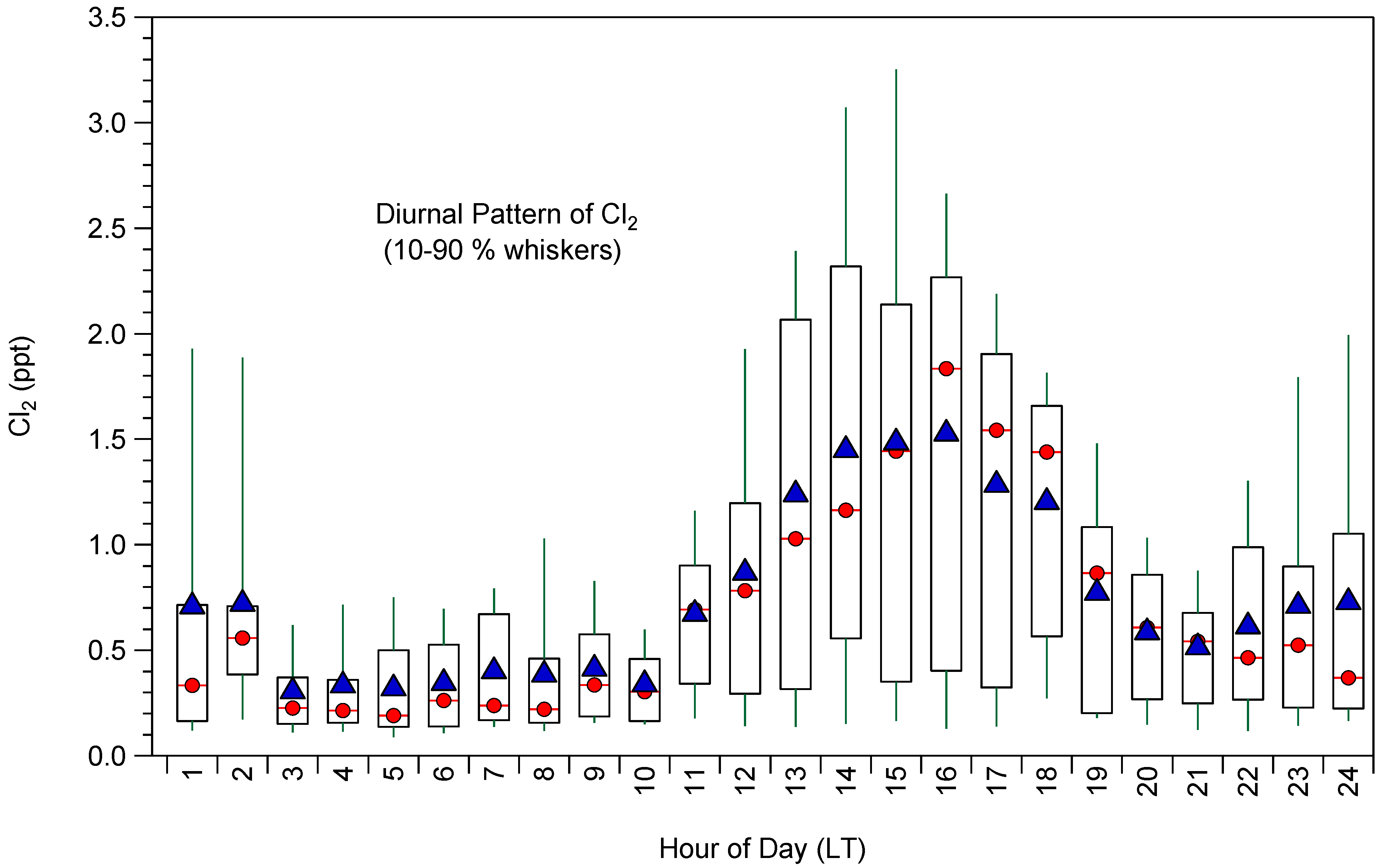
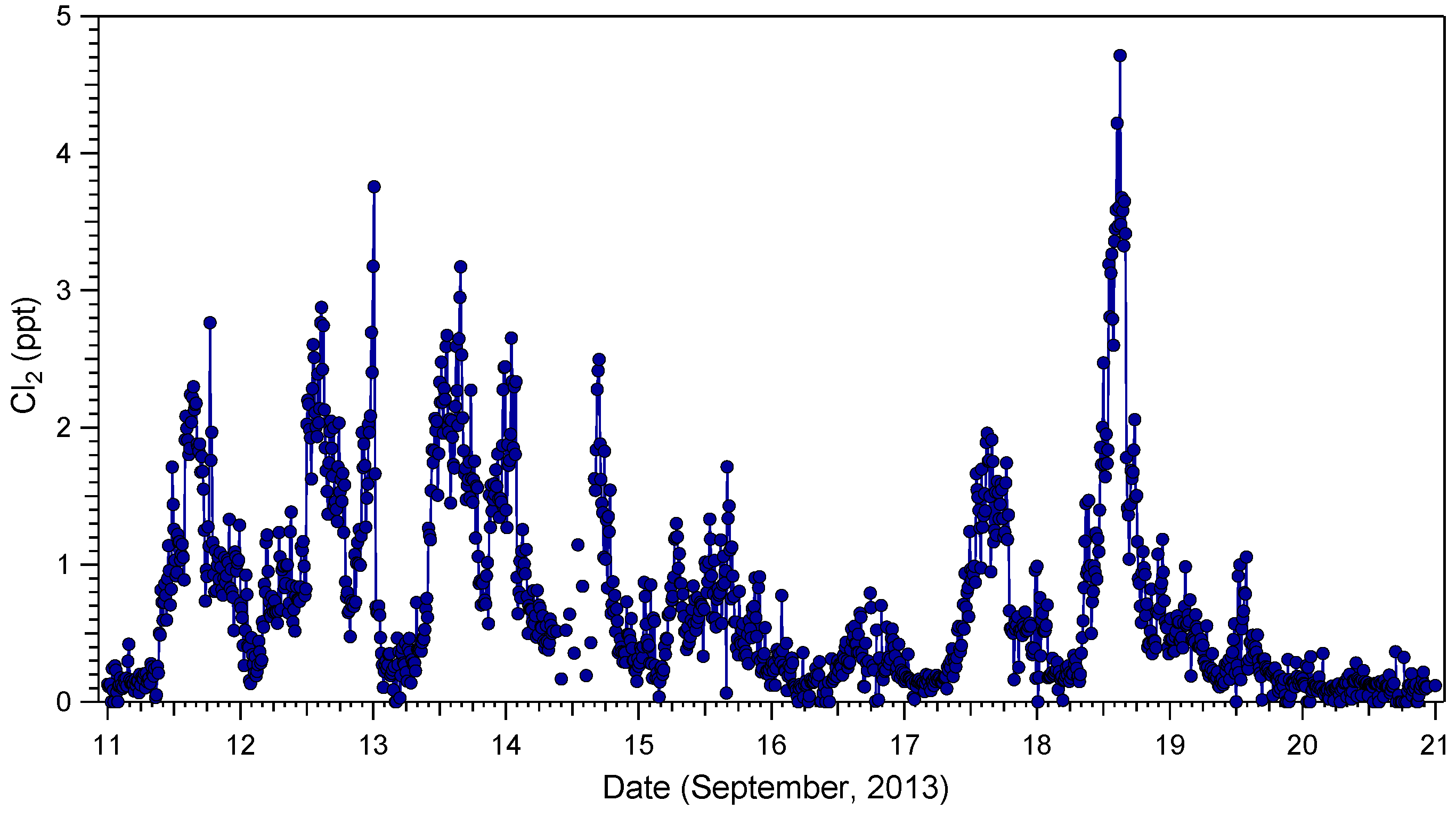
2.1. Cl2 Measurements

Concentrations of Cl2 typically peaked in the afternoon at concentrations ranging 1–10 ppt. During the afternoon hours (12:00–6:00 p.m.) on many days, Cl2 concentrations remained above 1–2 ppt. On most days, Cl2 peaked between 3:00 p.m. and 4:00 p.m. (Figure 1). Figure 3 shows the diurnal pattern of Cl2 concentrations between 11–21 September.
Figure 3. Diurnal pattern of Cl2 concentrations observed from 11–21 September. Concentrations were typically elevated in the mid to late afternoon, with a lower enhancement late at night due to late night peaks such as the night of 12 and 13 September. Boxes indicate 25th and 75th percentiles, and whiskers indicate 10th and 90th percentiles.
Atmosphere 06 01487 g003
These observed concentrations are slightly lower than concentrations observed in previous studies [22,23,24,58], and significantly lower than concentrations that have been detected in the arctic marine boundary layer [24,25]. However, the higher concentrations of Cl2 in these previous studies would be expected since they were taken in coastal areas, in close proximity to a large sea salt source. Although the Cl2 concentrations reported here are relatively low compared to other studies, the observation of a sustained concentration in spite of the rapid day-time photolysis of Cl2 suggests a significant source of Cl2 is present. For example, the average Cl2 concentration between 2:00 p.m. and 2:30 p.m. on 18 September was 3.8 ppt. The calculated photolysis rate constant for this same period, using the coordinates of the measurement site, was 2.5 × 10⁻³ s−1. This implies an approximate Cl2 photolysis rate of 35 ppt Cl2∙h−1 for a mid-day Cl2 concentration of 4 ppt Cl2; calculated 30-min average photolysis rates between 10:00 a.m. and 4:00 p.m. ranged from 7–35 ppt Cl2·h−1. Considering that concentrations on 18 September steadily increased from 10:00 a.m. and peaked at 2:00 p.m., this suggests that a minimum source strength of approximately 10–30 ppt∙h−1 during the mid-day is necessary to explain the observations. This is similar in strength to sources suggested by previous studies to explain Cl2 observations elsewhere [22,23].
Similar daytime Cl2 concentrations were observed for several other days during the campaign (Figure 1), suggesting that a similar source was present during those times as well. Such a Cl2 source could potentially lead to the enhanced oxidation of CH4 and other VOCs [23,25,58], and therefore enhanced formation of secondary organic aerosol. Additionally, enhanced O3 production can result from the presence of a Cl source [1,33]. The implications of this are discussed further in Section 2.4.
On several occasions (13–15 September, for example), increases in Cl2 were observed late at night or in the early morning, coinciding with increases in ClNO2. No significant anthropogenic emissions of gas phase Cl2 were known to be present in the area at the time. It is possible that the source of Cl2 in these situations was the same as ClNO2 since N2O5 has been shown to oxidize directly to Cl2 when particles are acidic [43]. Recent measurements in inland regions suggest that soil deflation could possibly play a larger role as a particulate chloride source than previously assumed [59,60,61]. Considering the diurnal pattern of Cl2, with peak concentrations occurring in the mid-afternoon, it is more likely that Cl2 is produced inland. Gas phase Cl2 transported from the coast would be degraded by photolysis by the time it reaches the measurement site, which could take several hours. Additionally, the heterogeneous production of reactive chlorine is thought to be driven by O3 or OH, species which peak during the mid-day. The timing of peak Cl2 concentrations thus suggest a heterogeneous mechanism as a possible source of observed Cl2.

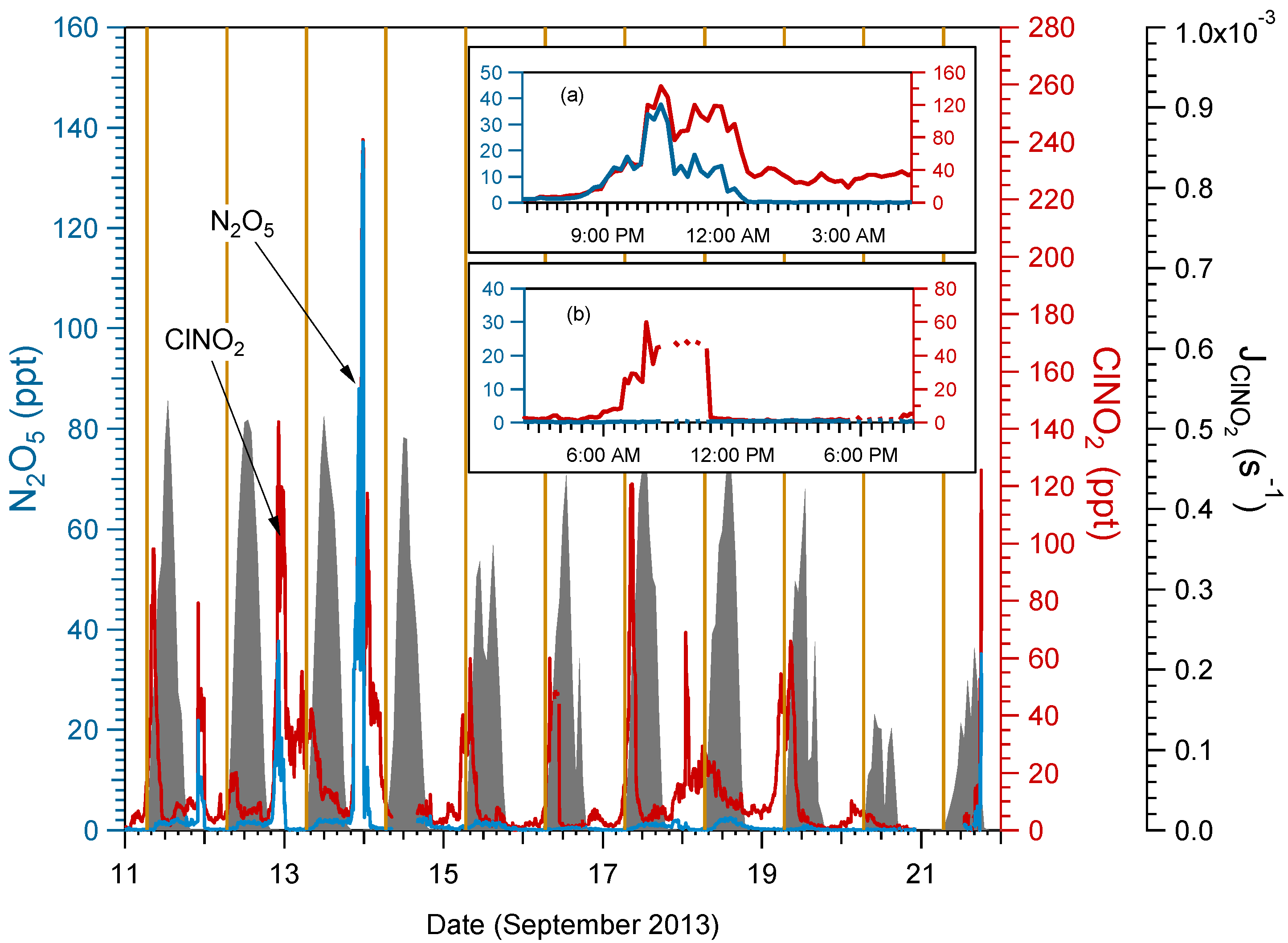
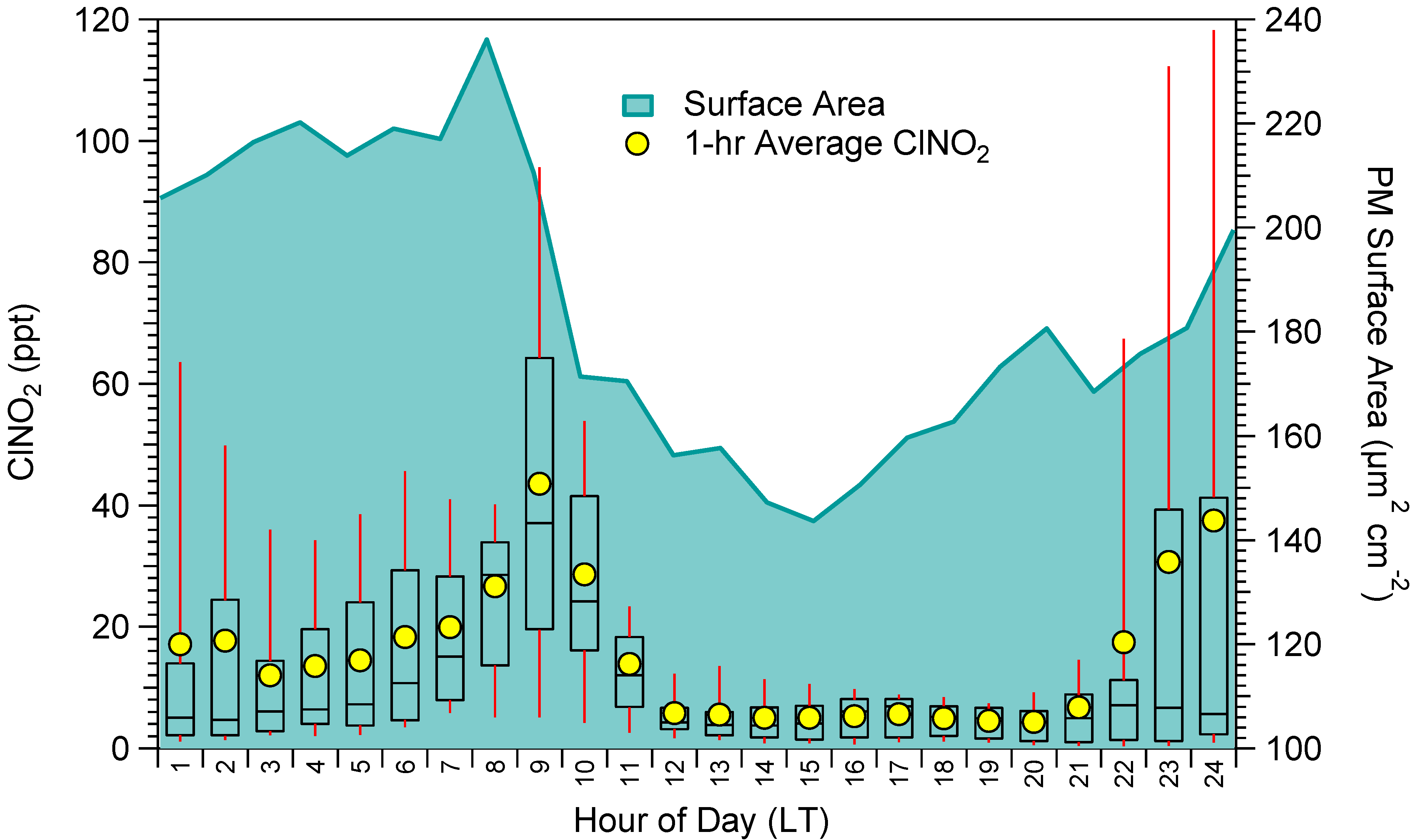
2.2. ClNO2 and N2O5 Measurements

For the month of September, 2013, ClNO2 was frequently detected at concentrations exceeding 50 ppt (approximately 40% of the days in the month). Observations for the period spanning 11–21 September are shown in Figure 2. Although the timing of peak ClNO2 concentration varied between days (e.g., Figure 2a compared to Figure 2b), the typical pattern was a peak ClNO2 concentration between 25–60 ppt occurring between 7:00–10:00 a.m. Daily 1-hour maximum concentrations averaged 24 ppt over the course of the month. On several days, however, ClNO2 concentrations peaked at night between 23:00–24:00, reaching concentrations over 100 ppt by midnight. Examples of such episodes can be seen in Figure 2 on the nights of 13 and 14 September. Observations of N2O5 were also made, and during periods when the concentration was high (11–13 September), N2O5 correlated well with ClNO2. However, there were many days (e.g., 14–21 September) during which elevated concentrations of ClNO2 were observed while N2O5 remained low or was below the detection limit, perhaps suggesting that ClNO2 production was limited by N2O5 on these days.
Observed concentrations of ClNO2 were lower than previous measurements made in coastal areas. During the Texas Air Quality Study II (TexAQS II), ClNO2 concentrations reaching 1200 ppt were detected in the Houston Ship Channel [37]. At another coastal location, in Los Angeles, CA, concentrations up to 1500 ppt were detected off the California coast in the Los Angeles region [24]. The lower magnitude of ClNO2 concentrations reported here is likely due to the fact that measurements were taken further inland (~125 km from the coast) and therefore further from a sea salt chloride source. However, the ClNO2 concentrations observed in Conroe, TX, USA, are also lower than recent observations much further from the coast. For example, ClNO2 concentrations of up to 800 ppt and 450 ppt were detected at Kohler Mesa, CO (~1400 km from coast) [46] and Hessen, Germany (~380 km from coast) [45], respectively. The most likely explanation for these observations is that an inland source of chloride was present at these locations, and more recent work [59] suggest the presence of a significant soil source for chloride in Colorado. In this study, the measurements are consistent with the influence of a moderate particulate chloride source, and the observation that N2O5 was never present in the absence of ClNO2 suggests that heterogeneous production was limited by N2O5 availability. The concentrations reported here are within the range predicted by previous modeling studies of ClNO2 production in the region [39,40,42]. Concentrations of this magnitude were predicted to result in an enhancement of O3 production up to several ppb [42].
On nights when ClNO2 and N2O5 correlated well, the concentrations typically peaked around midnight (Figure 2a). However, when elevated ClNO2 was present in the absence of N2O5, the concentrations typically peaked in the early to mid-morning (Figure 2b). Figure 4 shows a diurnal pattern of ClNO2 and PM2.5 surface area (as measured by the SEMS). Within the diurnal cycle of ClNO2 at the measurement site, two distinct patterns of ClNO2 concentrations are clearly visible. One pattern peaks early in the morning between 8 and 9 a.m., shortly after sunrise. In the other, late night ClNO2 peaks are observed around midnight, coinciding with peak N2O5 concentrations (11–13 September). The peak 1-h average particulate surface area also occurs around the time of peak ClNO2 concentrations in the early mornings, suggesting that conditions are favorable for the heterogeneous production of ClNO2 from N2O5 in air masses that are advected to the site in the early mornings.
Figure 4. Diurnal cycle of ClNO2 concentrations, showing two distinct patterns that are present during the campaign: (1) an early morning peak concentrations where ClNO2 is advected to the site, and (2) late night peak concentrations, when ClNO2 and N2O5 concentrations correlate significantly, suggesting more local inland production of ClNO2.
Atmosphere 06 01487 g004
Analysis of ACSM data collected during DISCOVER-AQ suggests high concentrations of particulate organic nitrates [62], which are formed either from photo-oxidation of hydrocarbons in the presence of NOx or from the reactions of hydrocarbons with NO3 radicals. Nitrate radical chemistry acts as a NOy sink, reducing the formation of N2O5 and therefore ClNO2 and could be responsible for relatively low N2O5 concentrations observed throughout most of the campaign.

2.3. Air Source Regions and Back Trajectories

On several days during the campaign, differences in the correlation of ClNO2 and N2O5 concentrations and the timing of ClNO2 peak concentrations suggest possible differences in the production and transport of ClNO2. To investigate this difference further, HYSPLIT back trajectories were calculated for each case [63]. Starting height was set to 70 m, the end point of the back trajectories was set to the coordinates of the Conroe field site, and the end time was set to the time of maximum observed ClNO2 concentration on each night. The model was used to generate a new back trajectory every two hours from the start time for a total of six 24-h back trajectories for each time period. Figure 5 shows a comparison of calculated back trajectories for the 13th and 16th of September.
Figure 5. A comparison of HYSPLIT back trajectories for the days shown in the insets of Figure 2. Left: Back trajectories for the morning of 13 September 2013. The back trajectories ending at the time of peak ClNO2 concentrations (10–11 p.m.) show air that originated inland near the TX-LA border 24 hours prior. Right: Back trajectories for the morning of 16 September 2013. The back trajectory at the time of peak ClNO2 concentration (7–8 a.m.) indicates that the air mass originated in the Gulf of Mexico 24 hours prior, passing between the Houston, TX region and the LA-TX border.
Atmosphere 06 01487 g005
One major difference between the two back trajectories is the amount of time that the air mass spent over land or over sea prior to arriving at the site. For example, air that was sampled at the site on 15–16 September originated in the Gulf of Mexico, resulting in a lower residence time over industrialized regions relative to the air sampled on the night of 12–13 September. Observations on the night of the 15th of September indicated very low N2O5. Elevated morning-time concentrations of ClNO2 in these scenarios (e.g., 15–17 September) most likely resulted from transport of ClNO2 to the measurement site from the Gulf Coast. ClNO2 concentrations of up to 1.2 ppb were previously detected along the coast [37] where HYSPLIT back trajectories indicate the air originated on 16 September (Figure 5). The lack of a corresponding increase in N2O5 concentrations during these early morning episodes also suggests that the ClNO2 observed at these times is produced elsewhere. The total amount of ClNO2 transported to the site on these mornings was probably limited by N2O5 availability since SEMS data indicate that the highest measured particulate surface area concentrations were observed during these times (Figure 4).
In contrast to the early morning peak concentrations, the air that was sampled on the night of 12 September originated inland, and the majority of its path was over land. On the night of 12 September, it might be expected that the observed air mass had been exposed to additional inland NOx sources that would explain the higher N2O5 concentration relative to the night of 15–16 September.
On several occasions, ClNO2 was found to be elevated in the afternoon during daylight hours. Examples of this include the afternoons of 12, 13 and 17 September. Back trajectories for the afternoon hours on these days indicate that air transported to the site originated along the Gulf coast. On the afternoon of 12 September between the hours of 1 and 5 p.m., incoming air originated along the gulf coast 18 hours prior to arriving at the site. The back trajectories for 13 and 17 September indicate that the air masses originated from the same region, frequently crossing the region between Lake Charles, LA and Houston, TX. The amount of ClNO2 that would need to be produced in the transported air can be estimated. For example, ClNO2 concentrations on the afternoons of 12 and 13 September were approximately 10–15 ppt. An air mass arriving at 2 p.m. would have been exposed to daylight for approximately 7 hours. Taking the average observed photolysis rate of ClNO2 between 7 a.m. and 2 p.m. for these dates, this corresponds to an average ClNO2 photolysis rate of 2.8 × 10⁻⁴ s−1. This suggests that approximately 1–2 ppb of ClNO2 would need to be produced in the incoming air masses during transport to the site in order for concentrations on the order of 10 ppt to be observed. Previous measurements and modeling predictions in this region indicate that elevated concentrations of ClNO2 can reach concentrations of this magnitude [37,39,40,42].
Back trajectories in the afternoons when Cl2 concentrations were typically elevated indicate that air is transported directly from the Gulf of Mexico, often passing over the metropolitan area of Houston, TX, USA. For example, air sampled at the site between 12–5 p.m. on the afternoon of 12, 13, 16 and 18 September consistently originated from the Gulf of Mexico 12 to 18 hours before being sampled. The transport of these air masses from the coast could suggest that long range sea salt transport contributed as a source of heterogeneously produced Cl2 at the site.

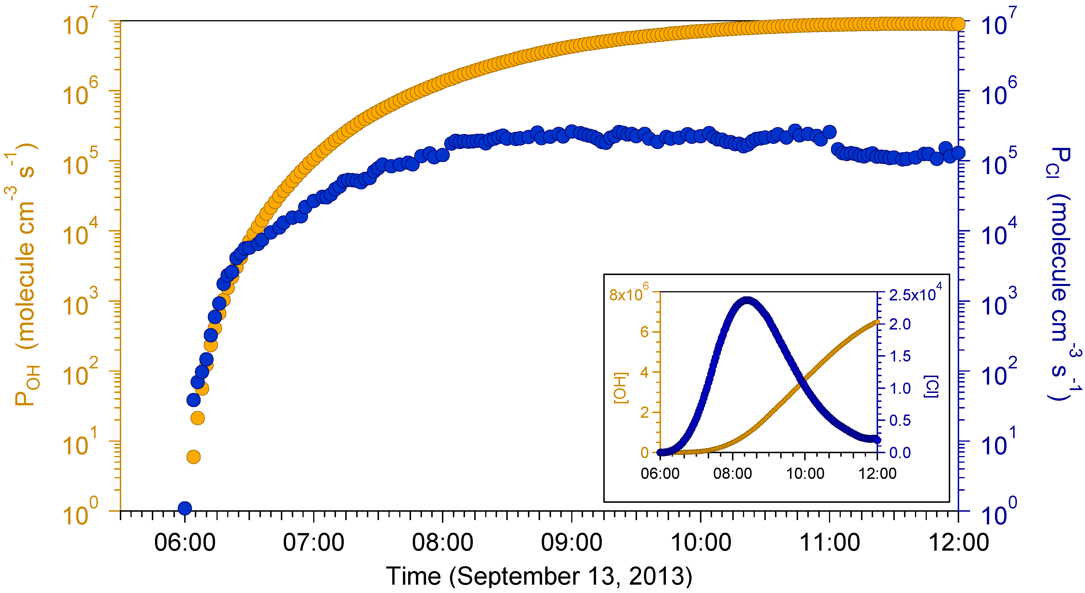
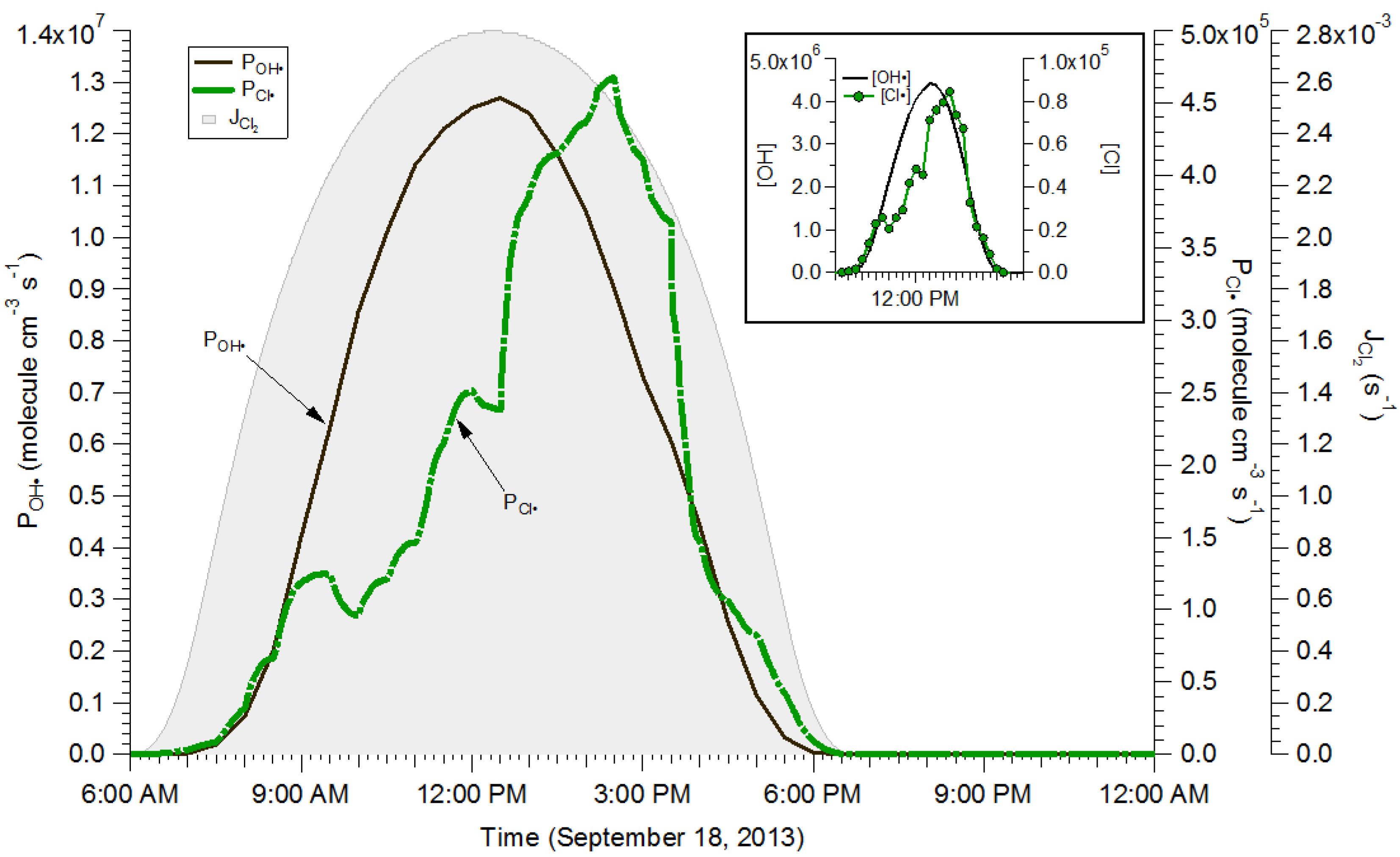
2.4. Box Modeling Results

The contribution of observed Cl2 and ClNO2 to Cl• production and resulting atmospheric reactivity were analyzed using ambient box modeling. The Statewide Air Pollution Research Center (SAPRC) software was used in combination with an updated version of the Carbon Bond 6 (CB6r2) chemical kinetics mechanism [64,65]. The CB6r2 mechanism was modified to include basic gas phase chlorine chemistry [65,66] in addition to Cl2 and ClNO2 photolysis in a manner similar to Sarwar et al. [39]. A list of reactions that were added is provided in the supplementary material. The photolysis rate of Cl2 was calculated internally to the mechanism for a latitude and longitude matching the location of the measurement site. For the dates used in the simulations, this resulted in a peak j C l 2 of 2.8 × 10⁻² s−1, occurring at 12:30 p.m. Deposition was not included and boundary layer height was fixed for the duration of the model run.
Conditions on 18 September were modeled in order to assess the effects of Cl2 on atmospheric reactivity. Although this day did not have the highest concentration of Cl2 observed throughout the campaign (Figure 1), sustained concentrations over 2 ppt were observed for the entire period between 12:00–6 p.m., suggesting a continuous source of Cl2 was present. Emissions of Cl2 were added to the model so that the observed Cl2 concentration profile was replicated in the simulations. On this day, relative humidity was 98% at 6:00 a.m., dropping to a minimum of 43% by 2:00 p.m., and temperature rose from 294 K at 6:00 am to 308 K at 2:00 p.m. Initial concentrations included 0.4 ppt Cl2, 8 ppb NO2, and 10 ppb O3, consistent with early morning observations at the site on 18 September. Using these initial conditions and meteorological inputs, the production of OH radicals was calculated Equation (1), and day-time OH production ranged 106–107 molecules∙cm−3 s−1. A typical urban VOC mixture [67] was included in simulations at a concentration of 20 ppbC. Four scenarios were simulated: (1) no Cl2 and no VOCs, (2) including Cl2 emissions, no VOCs, (3) no Cl2 emissions with 20 ppbC VOCs and (4) including Cl2 emissions and 20ppbC VOCs. Cl production was calculated from the photolysis of measured Cl2 concentrations Equation (2); an average emissions rate of 15 ppt∙h−1 between 8:00 a.m.–6:00 p.m. was found to be necessary to replicate the observed concentrations. A comparison of modeled OH and Cl production rates and concentrations are shown in Figure 6.
Figure 6. Production of OH and Cl radicals in a box modeling simulations for the conditions on 18 September 2013. The inset shows calculated concentrations of OH and Cl radicals in molecules∙cm−3·s−1.
Atmosphere 06 01487 g006
Although Cl production rates and concentrations are approximately 1–2 orders of magnitude lower than those of OH, the calculated concentrations are significant when the relative reactivity of the two radicals is taken into account. The rate constants for the reactions of Cl with many VOCs is significantly (up to 100 times) faster than the corresponding reactions of OH [9,10,11,68,69]. Thus, Cl concentrations on the order of 105 molecules∙cm−3 s−1 represent a significant radical source with respect to the oxidation of VOCs. For example, taking the maximum Cl concentration (8.5 × 10⁴ molecules∙cm−3) and the corresponding OH concentration at the same time (3.6 ×10⁶ molecules∙cm−3), the rate constant for the reaction of Cl and OH with CH4 at 298 K are approximately 1.0 × 10⁻¹³ and 6.4 × 10⁻¹⁵ cm3 molecules−1 s−1, respectively. Assuming a CH4 concentration of 1700 ppb, this corresponds to rates of reaction with CH4 for Cl and OH of 3 × 10⁵ and 8 × 10⁵ molecules∙cm−3 s−1, respectively. These rates of reaction indicate that the Cl from observed concentrations of Cl2 could significantly contribute to atmospheric reactivity with respect to VOC oxidation. It is also important that Cl2 and Cl peak in the mid to late afternoon when OH production begins to wane.
Measured O3 concentrations on the morning of 18 September were low with concentrations reaching around 5 ppb at 6:00 a.m. Simulations under-predicted day-time O3 concentrations by over 25% compared to measurements. Transport of O3 to the site in the afternoon (which is not included in this box modeling simulation) likely leads to higher observed O3 concentrations. O3 production was found to be enhanced by Cl2. The addition of Cl2 without VOC (model scenario 1 vs. 2) increased maximum modeled O3 concentration between 8:00 a.m.–6:00 p.m. by 10% (1 ppb) and RO2 concentration by up to 50% (1.1 ppt). The addition of Cl2 in the presence of VOC (model scenario 3 vs. 4) increased the maximum day-time O3 concentration by 8% (2 ppb) and RO2 concentration by 28% (10 ppt). These results are summarized in Table 1.
Conditions on the morning of 13 September (scenario 5 and 6) and 16 September (scenarios 7 and 8) were modeled in order to assess the effects of ClNO2 on atmospheric reactivity. Relative humidity and temperature in the model were set to approximate conditions present at the Conroe site. The simulation start time was set to midnight in order to capture the changes in radical production between nocturnal and early morning conditions. Model inputs for 13 September also included initial concentrations of 35 ppb O3 and 20 ppb NOx (consistent with measurements), as well as 20 ppbC VOC. A base case model run was performed without ClNO2 (scenario 5) and compared to the model run with 40 ppt initial ClNO2 (scenario 6). Model inputs for 16 September included initial concentrations of 15 ppb O3 and 10 ppb NOx (consistent with measurements), as well as 20 ppbC VOC. A base case with no ClNO2 (scenario 7) was compared to a separate model run (scenario 8), where initial ClNO2 concentrations were set to 0, and ClNO2 emissions were added to gradually increase the total amount of ClNO2 from 0 to 50 ppt between 6–8 a.m. (Figure 2b).
A comparison of the radical production rates of OH and Cl resulting from measured ClNO2, O3 and H2O concentrations is shown in Figure 7. Although Cl production reaches a peak rate that is approximately 2 orders of magnitude lower than peak OH production, its production in the early morning increases atmospheric reactivity during a time when OH concentrations are low. Concentrations of Cl peak in the very early morning (Figure 7 inset), approximately two hours before OH concentrations begin to increase. Using the peak modeled Cl concentration (2.5 × 10⁴ molecules∙cm−3 and an approximate OH concentration from the same time period (1.5 × 10⁶ molecules∙cm−3), the reaction rates with 1700 ppb CH4 are similar at 1.1 × 10⁵ and 4.1 × 10⁵ molecules∙cm−3 s−1 for Cl and OH, respectively.
Figure 7. OH production resulting from the photolysis of O3 compared to Cl production from observed concentrations of ClNO2 on the morning of 13 September 2013. The inset shows a comparison of modeled Cl and OH radical concentrations (molecules∙cm−3) during the same time period, assuming an initial ClNO2 concentration of 40 ppt (model scenario 6).
Atmosphere 06 01487 g007
The inclusion of 40 ppt ClNO2 enhanced O3 and RO2 concentrations between 7:00 a.m.–3:00 p.m. by a maximum of 6.5% and 0.4%, respectively, when compared to a simulation with no ClNO2 (scenarios 5 and 6 in Table 1). For simulations on the morning of 16 September, which included emissions of 50 ppt ClNO2 in the early morning, similar enhancements in O3 and RO2 concentrations were observed: in the presence of 20 ppbC VOC, O3 and RO2 concentrations were enhanced by 11.5% and 1.0%, respectively, when compared to a base case simulation without ClNO2 (scenarios 7 and 8 in Table 1). In the absence of VOCs the addition of ClNO2 did not significantly increase O3 or RO2 concentrations (not listed in Table 1). The increases in RO2 exemplify how ClNO2 at the observed concentrations can contribute significantly to atmospheric reactivity, particularly in the morning. A summary of these modeling results and the results of Cl2 simulations are listed in Table 1.
Table 1. Summary of Modeling Results.
ScenarioChlorine SpeciesComparison[VOC] (ppbC)∆[O3]max (%)∆[RO2]max (%)
1--101050
2Cl20
3--220828
4Cl220
5--32060.4
6ClNO220
7--420121
8ClNO220

3. Experimental Section

The area surrounding the air-quality monitoring station at Conroe, TX is primarily affected by pollution in the outflow of air from Houston, which hosts significant energy and petrochemical industries in addition to a large urban population. The regional atmospheric chemistry is also influenced by marine air from the Gulf of Mexico. The site itself is located in the middle of a field adjacent to the airport, with a gravel parking lot nearby and bordered by trees approximately 200 m to the North.
A permanent Texas Commission on Environmental Quality (TCEQ) ambient measurement station exists at this site and provided continuous meteorological data (wind speed, wind direction, temperature and relative humidity) for the duration of the campaign. NOx and O3 monitors were also present at the TCEQ site. During DISCOVER-AQ a temporary ground site was set up adjacent to the permanent station. Chlorine species were detected using a High Resolution Time-of-Flight Chemical Ionization Mass Spectrometer (HR-ToF-CIMS, henceforth referred to as CIMS) [70,71,72,73], which was operated in negative ionization mode utilizing the iodide reagent ion. Similar CIMS techniques have been used in previous studies for the detection of ClNO2, N2O5 and Cl2 [24,35,37,45,46,47,74,75], and other studies have described in detail the operation and application of the Aerodyne CIMS. Species reported here that were detected with the iodide CIMS included ClNO2, Cl2 and N2O5; the ions monitored for these species were IClNO2, ICl2, and IN2O5.
A sample flow of 2 LPM was introduced into the instrument through a ¼” outer diameter perfluoroalkoxy (PFA) Teflon® sample line connected to the stainless steel inlet by a ¼” to 10 mm stainless steel Swagelok union. The sample flow then passed into the ion-molecule reaction (IMR) chamber of the instrument, where it was mixed with a reagent ion flow of 2 LPM. Ionization in the IMR took place at a pressure of 200 mbar and temperature of 34°C (controlled by an IMR heater). I(H2O)n reagent ions were generated by passing a flow of ultra-high purity (UHP) N2 over a methyl iodide (CH3I, Sigma Aldrich, 99%) permeation tube. The N2 flow first passed through purified water (Milli-Q, model Advantage-A10) upstream of the CH3I permeation tube in order to provide the humidity necessary for sufficient production of H2OI ions. This also helped to stabilize the relative humidity within the IMR and resulting variations in sensitivity that have been noted for iodide chemical ionization [35,72]. Inside of the inlet, the sample flow then passed through 44.5 mm of the 10 mm outer diameter stainless steel tubing before passing through a critical orifice into the IMR. After mixing in the IMR the combined reagent and sample flow passed through two quadrupoles before entering the Time-of-Flight (ToF) mass analyzer. During the entire measurement period, the ToF was operated in V mode, providing higher sensitivity but lower resolution than W mode.
In order to test for measurement artifacts a flow of ultra-high purity (UHP) N2 was periodically introduced into the sampling inlet. This flushing of the sampling line resulted in a rapid drop to background levels in the signals for Cl2, N2O5 and ClNO2, suggesting that adsorption and subsequent desorption of these species from the inlet line walls was not a significant source of measurement artifacts. When the sampling commenced afterwards ion signals returned rapidly to ambient levels, suggestive of a high transmission efficiency. No explicit tests were performed to assess the N2O5 transmission efficiency in the field introducing uncertainty in the quantification of N2O5 which could be lost irreversibly to the inlet walls. The N2O5 concentrations in this study are reported assuming that transmission efficiency was equivalent to that observed during calibrations. We estimate that this introduces a measurement uncertainty of 20%, a conservative estimate compared to previous work [76] which cited a ± 7% accuracy for N2O5 measured using a different instrument.
Equations (1) and (2) were used to calculate the production of Cl and OH consistent with box modeling simulation results. The production of OH was calculated from the reactions of O(1D) with H2O, N2, and O2 (Equation (1)), in a manner similar to a previous observational study [45]. The rate of O3 photolysis was used to calculate the rate of O(1D) generation, and additional details on the derivation of Equation (1) are described in the supplementary material. The production of Cl proceeded directly from the photolysis of Cl2 (Equation (2)).
P O H =   2 J ( O 3 ) [ O 3 ] k H 2 O [ H 2 O ] / ( k H 2 O [ H 2 O ] +   k N 2 [ N 2 ]   +   k O 2 [ O 2 ] )
P C l = 2   ×   j C l 2 [ C l 2 ]
Additional simulations were performed to assess the impact of observed ClNO2 concentrations on Cl production and atmospheric reactivity, and Equation (3) was used to quantify the production of Cl from ClNO2.
P C l =   j C l N O 2 [ C l N O 2 ]

4. Conclusions

During the month of September 2013, concentrations of Cl2 and ClNO2 regularly reached or exceeded 2 ppt and 60 ppt, respectively, at an inland monitoring site in Southeast Texas. The concurrent presence or absence of N2O5 at the site depended on the source of the sampled air, and longer paths over land corresponded to higher concentrations of N2O5. Peak ClNO2 concentrations in the early mornings when little to no N2O5 was present on some days suggest that the production and transport of ClNO2 from a non-local source is occurring. Contemporaneous measurements of PM surface area suggest conditions favorable to heterogeneous conversion of N2O5 in the advected air masses on these mornings. The presence of Cl2 and ClNO2 at the site are significant due to their role as Cl sources. Although Cl2 concentrations are lower in magnitude, the fact that Cl2 concentrations consistently peak in the afternoon when photolysis rates are highest suggests a Cl2 source of approximately 30 ppt∙h−1 Cl2. Box modeling simulations suggest that such concentrations can contribute to enhanced O3 and RO2 production during the day. The source of ClNO2 is likely the result of reactions between anthropogenic NOx sources and particulate chloride originating along the Gulf Coast, and the reported values are within the range of previous model predictions in the region. Assuming that the surface measurements made in the early morning are representative of the entire nocturnal boundary layer, ClNO2 was also found to contribute to Cl production and atmospheric reactivity, particularly in the early morning before significant OH production begins. Overall, the results suggest that Cl2 and ClNO2 affect atmospheric reactivity and can impact the formation of ozone and secondary organic aerosol. In a region where attainment of the National Ambient Air Quality Standard for ozone has been an issue in the past decades, quantifying the effects of reactive chlorine chemistry is important for assuring future attainment.

Supplementary Files

Supplementary File 1

Acknowledgments

This work was funded in part through a grant from the Texas Commission on Environmental Quality (TCEQ), administered by The University of Texas through the Air Quality Research Program (Project 12-012). The contents, findings opinions and conclusions are the work of the authors and do not necessarily represent findings, opinions or conclusions of the TCEQ. The work was also funded in part with funds from the State of Texas as part of the program of the Texas Air Research Center. The contents do not necessarily reflect the views and policies of the sponsor nor does the mention of trade names or commercial products constitute endorsement or recommendation for use. The authors would like to acknowledge the support of the entire DISCOVER-AQ Texas 2013 team. Code for the SAPRC box modeling software can be found at http://www.engr.ucr.edu/~carter/SAPRC. Meteorological data used for model input can be obtained via the TCEQ website (http://www.tceq.state.tx.us).

Author Contributions

Cameron Faxon, Jeffrey Bean, and Lea Hildebrandt Ruiz planned, prepared and conducted the ambient measurements. Cameron Faxon conducted the box model simulations and analyzed ambient data and box model results presented in this work. The manuscript was written by Cameron Faxon with the guidance of Lea Hildebrandt Ruiz.

Conflicts of Interest

The authors declare no conflict of interest.

References

  1. Tanaka, P.L.; Riemer, D.D.; Chang, S.; Yarwood, G.; McDonald-Buller, E.C.; Apel, E.C.; Orlando, J.J.; Silva, P.J.; Jimenez, J.L.; Canagaratna, M.R.; et al. Direct evidence for chlorine-enhanced urban ozone formation in Houston, Texas. Atmos. Environ. 2003, 37, 1393–1400. [Google Scholar] [CrossRef]
  2. Wang, L.; Thompson, T.; McDonald-Buller, E.C.; Allen, D.T. Photochemical modeling of emissions trading of highly reactive volatile organic compounds in Houston, Texas. 2. Incorporation of chlorine emissions. Environ. Sci. Technol. 2007, 41, 2103–2107. [Google Scholar] [CrossRef] [PubMed]
  3. Faxon, C.B.; Allen, D.T. Chlorine chemistry in urban atmospheres: A review. Environ. Chem. 2013, 10, 221–233. [Google Scholar] [CrossRef]
  4. Wingenter, O.W.; Sive, B.C.; Blake, N.J.; Blake, D.R.; Rowland, F.S. Atomic chlorine concentrations derived from ethane and hydroxyl measurements over the equatorial Pacific Ocean: Implication for dimethyl sulfide and bromine monoxide. J. Geophys. Res. 2005, 110. [Google Scholar] [CrossRef]
  5. Graedel, T.E.; Keene, W.C. Tropospheric budget of reactive chlorine. Glob. Biogeochem. Cycles 1995, 9, 47–77. [Google Scholar] [CrossRef]
  6. Keene, C.; Aslam, M.; Khalil, K.; Erickson, J.; Archie, I.I.I.; Graedel, E.; Loberr, M.; Aucott, M.L.; Ling, S.; Harper, D.B.; et al. Composite global emissions of reactive chlorine from anthropogenic and natural sources : Reactive chlorine emissions inventory. J. Geophys. Res. 1999, 104, 8429–8440. [Google Scholar] [CrossRef]
  7. Sarwar, G.; Bhave, P.V. Modeling the effect of chlorine emissions on ozone levels over the eastern United States. J. Appl. Meteorol. Climatol. 2007, 46, 1009–1019. [Google Scholar] [CrossRef]
  8. Liu, C.L.; Smith, J.D.; Che, D.L.; Ahmed, M.; Leone, S.R.; Wilson, K.R. The direct observation of secondary radical chain chemistry in the heterogeneous reaction of chlorine atoms with submicron squalane droplets. Phys. Chem. Chem. Phys. 2011, 13, 8993–9007. [Google Scholar] [CrossRef] [PubMed]
  9. Wang, L.; Arey, J.; Atkinson, R. Reactions of chlorine atoms with a series of aromatic hydrocarbons. Environ. Sci. Technol. 2005, 39, 5302–10. [Google Scholar] [CrossRef] [PubMed]
  10. Nelson, L.; Rattigan, O.; Neavyn, R.; Sidebottom, H. Absolute and relative rate constants for reactions of hydroxyl radicals and chlorine atoms with series of aliphatic alcohols and ethers at 298K. Int. J. Chem. Kinet. 1990, 22, 1111–1126. [Google Scholar] [CrossRef]
  11. Aschmann, S.M.; Atkinson, R. Rate Constants for the Gas-Phase Reactions of alkanes with Cl atoms at 296. Int. J. Chem. Kinet. 1995, 27, 613–622. [Google Scholar] [CrossRef]
  12. Canosa-Mas, C.E.; Hutton-Squire, H.R.; King, M.D.; Stewart, D.J.; Thompson, K.C.; Wayne, R.P. Laboratory Kinetic Studies of the Reactions of Cl Atoms with Species of Biogenic Origin: Δ3-Carene, Methacrolein and Methyl Vinyl Ketone. J. Atmos. Chem. 1999, 34, 163–170. [Google Scholar] [CrossRef]
  13. Ragains, M.L.; Finlayson-Pitts, B.J. Kinetics and mechanism of the reaction of Cl atoms with 2-Methyl-1,3-butadiene (Isoprene) at 298 K. J. Phys. Chem. A 1997, 5639, 1509–1517. [Google Scholar] [CrossRef]
  14. Chang, S.; McDonald-Buller, E.; Kimura, Y.; Yarwood, G.; Neece, J.; Russell, M.; Tanaka, P.; Allen, D. Sensitivity of urban ozone formation to chlorine emission estimates. Atmos. Environ. 2002, 36, 4991–5003. [Google Scholar] [CrossRef]
  15. Tanaka, P.L.; Allen, D.T.; Mullins, C.B. An environmental chamber investigation of chlorine-enhanced ozone formation in Houston, Texas. J. Geophys. Res. 2003, 108. [Google Scholar] [CrossRef]
  16. Knipping, E.M.; Dabdub, D. Impact of chlorine emissions from sea-salt aerosol on coastal urban ozone. Environ. Sci. Technol. 2003, 37, 275–284. [Google Scholar] [CrossRef] [PubMed]
  17. Sander, S.P.; Friedl, R.R.; Barker, J.R.; Golden, D.M.; Kurylo, M.J.; Sciences, G.E.; Wine, P.H.; Abbatt, J.P.D.; Burkholder, J.B.; Kolb, C.E.; et al. Chemical Kinetics and Photochemical Data for Use in Atmospheric Studies: Evaluation Number 17. Available online: https://jpldataeval.jpl.nasa.gov/pdf/JPL%2010-6%20Final%2015Jun8011.pdf (accessed on 31 August 2015).
  18. Chang, S.; Allen, D.T. Chlorine chemistry in urban atmospheres: Aerosol formation associated with anthropogenic chlorine emissions in southeast Texas. Atmos. Environ. 2006, 40, 512–523. [Google Scholar] [CrossRef]
  19. Chang, S.; Tanaka, P.; Mcdonald-buller, E.; Allen, D.T. Emission inventory for atomic chlorine precursors in Southeast Texas. Available online: http://www.tceq.state.tx.us/assets/public/implementation/air/am/contracts/reports/oth/EmissioninventoryForAtomicChlorinePrecursors.pdf (accessed on 31 August 2015).
  20. Atkinson, R.; Baulch, D.L.; Cox, R.A.; Crowley, J.N.; Hampson, R.F.; Hynes, R.G.; Jenkin, M.E.; Rossi, M.J.; Troe, J. Evaluated kinetic and photochemical data for atmospheric chemistry: Volume III—Gas phase reactions of inorganic halogens. Atmos. Chem. Phys. 2007, 7, 981–1191. [Google Scholar] [CrossRef]
  21. Pszenny, A.A.P.; Keene, W.C.; Jacob, D.J.; Fan, S.; Maben, J.R.; Zetwo, M.P. Evidence of inorganic chlorine gases other than hydrogen chloride in marine surface air. Geopys. Res. Lett. 1993, 20, 699–702. [Google Scholar] [CrossRef]
  22. Spicer, C.; Chapman, E.; Finlayson-Pitts, B.; Plastrige, R.; Hubbe, J.; Fast, J.; Berkowitz, C. Unexpectedly high concentrations of molecular chlorine in coastal air. Nature 1998, 394, 353–356. [Google Scholar] [CrossRef]
  23. Finley, B.D.; Saltzman, E.S. Measurement of Cl2 in coastal urban air. Geophys. Res. Lett. 2006, 33. [Google Scholar] [CrossRef]
  24. Riedel, T.P.; Bertram, T.H.; Crisp, T.A.; Williams, E.J.; Lerner, B.M.; Vlasenko, A.; Li, S.M.; Gilman, J.; de Gouw, J.; Bon, D.M.; et al. A Nitryl chloride and molecular chlorine in the coastal marine boundary layer. Environ. Sci. Technol. 2012, 46, 10463–10470. [Google Scholar] [CrossRef] [PubMed]
  25. Liao, J.; Huey, L.G.; Liu, Z.; Tanner, D.J.; Cantrell, C.A.; Orlando, J.J.; Flocke, F.M.; Shepson, P.B.; Weinheimer, A.J.; Hall, S.R.; et al. High levels of molecular chlorine in the Arctic atmosphere. Nat. Geosci. 2014, 7, 91–94. [Google Scholar] [CrossRef]
  26. Chang, S.; Allen, D.T. Atmospheric chlorine chemistry in southeast Texas: impacts on ozone formation and control. Environ. Sci. Technol. 2006, 40, 251–262. [Google Scholar] [CrossRef] [PubMed]
  27. Oum, K.W.; Lakin, M.J.; DeHaan, D.O.; Brauers, T.; Finlayson-Pitts, B.J. Formation of molecular chlorine from the photolysis of ozone and aqueous sea-salt particles. Science 1998, 279, 74–76. [Google Scholar] [CrossRef] [PubMed]
  28. Herrmann, H.; Majdik, Z.; Ervens, B.; Weise, D. Halogen production from aqueous tropospheric particles. Chemosphere 2003, 52, 485–502. [Google Scholar] [CrossRef]
  29. Sadanaga, Y.; Hirokawa, J.; Akimoto, H. Formation of molecular chlorine in dark condition: Heterogeneous reaction of ozone with sea salt in the presence of ferric ion. Geophys. Res. Lett. 2001, 28, 4433–4436. [Google Scholar] [CrossRef]
  30. Knipping, E.M. Experiments and simulations of ion-enhanced interfacial chemistry on aqueous NaCl aerosols. Science 2000, 288, 301–306. [Google Scholar] [CrossRef] [PubMed]
  31. Behnke, W.; Zetzsch, C. Heterogeneous formation of chlorine atoms from various aerosols in the presence of O3 and HCl. J. Aerosol Sci. 1989, 20, 1167–1170. [Google Scholar] [CrossRef]
  32. Keene, W.C.; Pszenny, A.A.P.; Jacob, D.J.; Duce, R.A.; Galloway, J.N.; Schultz-Tokos, J.J.; Sievering, H.; Boatman, J.F. The geochemical cycling of reactive chlorine through the marine troposphere. Glob. Biogeochem. Cycles 1990, 4, 407–430. [Google Scholar] [CrossRef]
  33. Knipping, E.M. Modeling Cl2 formation from aqueous NaCl particles: Evidence for interfacial reactions and importance of Cl2 decomposition in alkaline solution. J. Geophys. Res. 2002, 107. [Google Scholar] [CrossRef]
  34. George, I.J.; Abbatt, J.P.D. Heterogeneous oxidation of atmospheric aerosol particles by gas-phase radicals. Nat. Chem. 2010, 2, 713–722. [Google Scholar] [CrossRef] [PubMed]
  35. Kercher, J.P.; Riedel, T.P.; Thornton, J.A. Chlorine activation by N2O5: Simultaneous, in situ detection of ClNO2 and N2O5 by chemical ionization mass spectrometry. Atmos. Measu. Tech. 2009, 2, 193–204. [Google Scholar] [CrossRef]
  36. Thornton, J.A.; Abbatt, J.P.D. N2O5 reaction on submicron sea salt aerosol: Kinetics, products, and the effect of surface active organics. J. Phys. Chem. A 2005, 109, 10004–10012. [Google Scholar] [CrossRef] [PubMed]
  37. Osthoff, H.D.; Roberts, J.M.; Ravishankara, a. R.; Williams, E.J.; Lerner, B.M.; Sommariva, R.; Bates, T.S.; Coffman, D.; Quinn, P.K.; Dibb, J.E.; et al. High levels of nitryl chloride in the polluted subtropical marine boundary layer. Nat. Geosci. 2008, 1, 324–328. [Google Scholar] [CrossRef]
  38. Roberts, J.M.; Osthoff, H.D.; Brown, S.S.; Ravishankara, A.R.; Coffman, D.; Quinn, P.; Bates, T. Laboratory studies of products of N2O5 uptake on Cl-containing substrates. Geophys. Res. Lett. 2009, 36. [Google Scholar] [CrossRef]
  39. Sarwar, G.; Simon, H.; Bhave, P.; Yarwood, G. Examining the impact of heterogeneous nitryl chloride production on air quality across the United States. Atmos. Chem. Phys. 2012, 12, 6455–6473. [Google Scholar] [CrossRef]
  40. Simon, H.; Kimura, Y.; McGaughey, G.; Allen, D.T.; Brown, S.S.; Coffman, D.; Dibb, J.; Osthoff, H.D.; Quinn, P.; Roberts, J.M. Modeling heterogeneous ClNO2 formation, chloride availability, and chlorine cycling in Southeast Texas. Atmos. Environ. 2010, 44, 5476–5488. [Google Scholar] [CrossRef]
  41. Simon, H.; Kimura, Y.; McGaughey, G.; Allen, D.T.; Brown, S.S.; Osthoff, H.D.; Roberts, J.M.; Byun, D.; Lee, D. Modeling the impact of ClNO2 on ozone formation in the Houston area. J. Geophys. Res. 2009, 114. [Google Scholar] [CrossRef]
  42. Sarwar, G.; Simon, H.; Xing, J.; Mathur, R. Importance of tropospheric ClNO2 chemistry across the Northern Hemisphere. Geophys. Res. Lett. 2014, 41, 4050–4058. [Google Scholar] [CrossRef]
  43. Roberts, J.M.; Osthoff, H.D.; Brown, S.S.; Ravishankara, A.R. N2O5 oxidizes chloride to Cl2 in acidic atmospheric aerosol. Science 2008, 321, 1059–1059. [Google Scholar] [CrossRef] [PubMed]
  44. Thomas, J.L.; Jimenez-Aranda, A.; Finlayson-Pitts, B.J.; Dabdub, D. Gas-phase molecular halogen formation from NaCl and NaBr aerosols: when are interface reactions important? J. Phys. Chem. A 2006, 110, 1859–1867. [Google Scholar] [CrossRef] [PubMed]
  45. Phillips, G.J.; Tang, M.J.; Thieser, J.; Brickwedde, B.; Schuster, G.; Bohn, B.; Lelieveld, J.; Crowley, J.N. Significant concentrations of nitryl chloride observed in rural continental Europe associated with the influence of sea salt chloride and anthropogenic emissions. Geophys. Res. Lett. 2012, 39. [Google Scholar] [CrossRef]
  46. Thornton, J.A.; Kercher, J.P.; Riedel, T.P.; Wagner, N.L.; Cozic, J.; Holloway, J.S.; Dubé, W.P.; Wolfe, G.M.; Quinn, P.K.; Middlebrook, A.M.; et al. A large atomic chlorine source inferred from mid-continental reactive nitrogen chemistry. Nature 2010, 464, 271–274. [Google Scholar] [CrossRef] [PubMed]
  47. Mielke, L.H.; Furgeson, A.; Osthoff, H.D. Observation of ClNO2 in a mid-continental urban environment. Environ. Sci. Technol. 2011, 45, 8889–8896. [Google Scholar] [CrossRef] [PubMed]
  48. Behnke, W.; George, C.; Scheer, V.; Zetzsch, C. Production and decay of ClNO2 from the reaction of gaseous N2O5 with NaCl solution: Bulk and aerosol experiments. J. Geophys. Res. 1997, 102, 3795–3804. [Google Scholar] [CrossRef]
  49. Behnke, W.; Krüger, H.-U.; Scheer, V.; Zetzsch, C. Formation of atomic Cl from sea spray via photolysis of nitryl chloride: Determination of the sticking coefficient of N2O5 on NaCl aerosol. J. Aerosol Sci. 1991, 22, S609–S612. [Google Scholar] [CrossRef]
  50. Frenzel, A.; Scheer, V.; Sikorski, R.; George, C.; Behnke, W.; Zetzsch, C. Heterogeneous interconversion reactions of BrNO2, ClNO2, Br2, and Cl2. J. Phys. Chem. A 1998, 102, 1329–1337. [Google Scholar] [CrossRef]
  51. Schweitzer, F.; Mirabel, P.; George, C. Multiphase chemistry of N2O5, ClNO2, and BrNO2. J. Phys. Chem. A 1998, 102, 3942–3952. [Google Scholar] [CrossRef]
  52. Bertram, T.H.; Thornton, J.A. Toward a general parameterization of N2O5 reactivity on aqueous particles: The competing effects of particle liquid water, nitrate and chloride. Atmos. Chem. Phys. Discuss. 2009, 9, 15181–15214. [Google Scholar] [CrossRef]
  53. Mielke, L.H.; Stutz, J.; Tsai, C.; Hurlock, S.C.; Roberts, J.M.; Veres, P.R.; Froyd, K.D.; Hayes, P.L.; Cubison, M.J.; Jimenez, J.L.; et al. Heterogeneous formation of nitryl chloride and its role as a nocturnal NOx reservoir species during CalNex-LA 2010. J. Geophys. Res. Atmos. 2013, 118, 10638–10652. [Google Scholar]
  54. Tham, Y.J.; Yan, C.; Xue, L.; Zha, Q.; Wang, X.; Wang, T. Presence of high nitryl chloride in Asian coastal environment and its impact on atmospheric photochemistry. Chin. Sci. Bull. 2013, 59, 356–359. [Google Scholar] [CrossRef]
  55. Riedel, T.P.; Wagner, N.L.; Dubé, W.P.; Middlebrook, A.M.; Young, C.J.; Öztürk, F.; Bahreini, R.; VandenBoer, T.C.; Wolfe, D.E.; Williams, E.J.; et al. Chlorine activation within urban or power plant plumes: Vertically resolved ClNO2 and Cl2 measurements from a tall tower in a polluted continental setting. J. Geophys. Res. Atmos. 2013, 118, 8702–8715. [Google Scholar] [CrossRef]
  56. National Aeronautics and Space Administration. Deriving Information on Surface Conditions from Column and Vertically Resolved Observations Relevant to Air Quality (DISCOVER-AQ). Available online: http://discover-aq.larc.nasa.gov/ (accessed on 31 August 2015).
  57. Ng, N.L.; Herndon, S.C.; Trimborn, a.; Canagaratna, M.R.; Croteau, P.L.; Onasch, T.B.; Sueper, D.; Worsnop, D.R.; Zhang, Q.; Sun, Y.L.; et al. An Aerosol Chemical Speciation Monitor (ACSM) for routine monitoring of the composition and mass concentrations of ambient aerosol. Aerosol Sci. Technol. 2011, 45, 780–794. [Google Scholar] [CrossRef]
  58. Finley, B.D.; Saltzman, E.S. Observations of Cl2, Br2, and I2 in coastal marine air. J. Geophys. Res. 2008, 113, 1–14. [Google Scholar]
  59. Jordan, C.E.; Pszenny, A.A.P.; Keene, W.C.; Cooper, O.R.; Deegan, B.; Maben, J.; Routhier, M.; Sander, R.; Young, A.H. Origins of aerosol chlorine during winter over north central Colorado, USA. J. Geophys. Res. Atmos. 2015, 120, 678–694. [Google Scholar] [CrossRef]
  60. Young, A.H.; Keene, W.C.; Pszenny, A.A.P.; Sander, R.; Thornton, J.A.; Riedel, T.P.; Maben, J.R. Phase partitioning of soluble trace gases with size-resolved aerosols in near-surface continental air over northern Colorado, USA, during winter. J. Geophys. Res. Atmos. 2013, 118, 9414–9427. [Google Scholar] [CrossRef]
  61. Pratt, K.A.; Prather, K.A. Aircraft measurements of vertical profiles of aerosol mixing states. J. Geophys. Res. Atmos. 2010, 115, 1–10. [Google Scholar] [CrossRef]
  62. Hildebrandt Ruiz, L.; Yarwood, G.; Koo, B.; Heo, G. Quality assurance project plan project 14-024—Sources of organic particulate matter in Houston: Evidence from DISCOVER-AQ data modeling and experiments. Available online: http://aqrp.ceer.utexas.edu/projectinfoFY14_15%5C14-024%5C14-024%20QAPP.pdf (accessed on 31 August 2015).
  63. Draxler, R.R.; Hess, G. Description of the HYSPLIT_4 Modeling System. Available online: https://ready.arl.noaa.gov/HYSPLIT.php; 2010 (accessed on 31 August 2015).
  64. Yarwood, G.; Jung, J.; Whitten, G.Z.; Heo, G.; Mellberg, J.; Estes, M. Updates to the Carbon Bond mechanism for version 6 (CB6). In Proceedings of the 9th Annual CMAS Conference, Chapel Hill, NC, USA, 11–13 October 2010; pp. 1–4.
  65. Yarwood, G.; Rao, S. Updates to the Carbon Bond Chemical Mechanism: CB05; RT-0400675; Final report to the US EPA; US EPA: Washington, DC, USA, 2005.
  66. Tanaka, P.L.; Allen, D.T.; McDonald-Buller, E.C.; Chang, S.; Kimura, Y.; Mullins, C.B.; Yarwood, G.; Neece, J.D. Development of a chlorine mechanism for use in the carbon bond IV chemistry model. J. Geophys. Res. 2003, 108. [Google Scholar] [CrossRef]
  67. Carter, W.P.L.; Luo, D.; Malkina, I.L.; Pierce, J.A. Environmental Chamber Studies of Atmospheric Reactivities of Volatile Organic Compounds: Effects of Varying Chamber and Light Source. 1995. Availavle online: https://www.cert.ucr.edu/~carter/pubs/explrept.pdf (accessed on 31 August 2015).
  68. Sokolov, O.; Hurley, M.D.; Wallington, T.J.; Kaiser, E.W.; Platz, J.; Nielsen, O.J.; Berho, F.; Rayez, M.T.; Lesclaux, R. Kinetics and mechanism of the gas-phase reaction of Cl atoms with benzene. J. Phys. Chem. A 1998, 102, 10671–10681. [Google Scholar] [CrossRef]
  69. Wingenter, O.W.; Blake, D.R.; Blake, N.J.; Sive, B.C.; Rowland, F.S.; Atlas, E.; Flocke, F. Tropospheric hydroxyl and atomic chlorine concentrations, and mixing timescales determined from hydrocarbon and halocarbon measurements made over the Southern Ocean. J. Geophys. Res. 1999, 104, 21,819–21,828. [Google Scholar] [CrossRef]
  70. Bertram, T.H.; Kimmel, J.R.; Crisp, T.A.; Ryder, O.S.; Yatavelli, R.L.N.; Thornton, J.A.; Cubison, M.J.; Gonin, M.; Worsnop, D.R. A field-deployable, chemical ionization time-of-flight mass spectrometer. Atmos. Meas. Tech. 2011, 4, 1471–1479. [Google Scholar] [CrossRef]
  71. Yatavelli, R.L.N.; Lopez-Hilfiker, F.; Wargo, J.D.; Kimmel, J.R.; Cubison, M.J.; Bertram, T.H.; Jimenez, J.L.; Gonin, M.; Worsnop, D.R.; Thornton, J.A. A chemical ionization high-resolution time-of-flight mass spectrometer coupled to a Micro Orifice Volatilization Impactor (MOVI-HRToF-CIMS) for analysis of gas and particle-phase organic species. Aerosol Sci. Technol. 2012, 46, 1313–1327. [Google Scholar] [CrossRef]
  72. Lee, B.H.; Lopez-Hilfiker, F.D.; Mohr, C.; Kurtén, T.; Worsnop, D.R.; Thornton, J.A. An iodide-adduct high-resolution time-of-flight chemical-ionization mass spectrometer: Application to atmospheric inorganic and organic compounds. Environ. Sci. Technol. 2014, 48, 6309–6317. [Google Scholar] [CrossRef] [PubMed]
  73. Aljawhary, D.; Lee, A.K.Y.; Abbatt, J.P.D. High-resolution chemical ionization mass spectrometry (ToF-CIMS): Application to study SOA composition and processing. Atmos. Meas. Tech. 2013, 6, 3211–3224. [Google Scholar] [CrossRef]
  74. Slusher, D.L.; Huey, L.G.; Tanner, D.J.; Flocke, F.M.; Roberts, J.M. A Thermal Dissociation-Chemical Ionization Mass Spectrometry (TD-CIMS) technique for the simultaneous measurement of peroxyacyl nitrates and dinitrogen pentoxide. J. Geophys. Res. 2004, 109. [Google Scholar] [CrossRef]
  75. Zheng, W.; Flocke, F.M.; Tyndall, G.S.; Swanson, A.; Orlando, J.J.; Roberts, J.M.; Huey, L.G.; Tanner, D.J. Characterization of a thermal decomposition chemical ionization mass spectrometer for the measurement of Peroxy Acyl Nitrates (PANs) in the atmosphere. Atmos. Chem. Phys. 2011, 11, 6529–6547. [Google Scholar] [CrossRef] [Green Version]
  76. Fuchs, H.; Dube, W.P.; Ciciora, S.J.; Brown, S.S. Determination of inlet transmission and conversion efficiencies for in situ measurements of the nocturnal nitrogen oxides, NO3, N2O5 and NO2, via pulsed cavity ring-down spectroscopy. Anal. Chem. 2008, 80, 6010–6017. [Google Scholar] [CrossRef] [PubMed]

