1. Introduction
Atmospheric aerosol particles play an important role in modulating the Earth’s radiation balance by scattering and absorbing incoming solar radiation [
1,
2]. Obtaining of aerosol properties with passive remote sensing requires confident identification and exclusion of potential cloud contamination. Such identification and exclusion—so-called cloud-screening—has received increased attention in the recent years. It has been applied when retrieving aerosol properties from ground-based measurements at both permanent and temporary sites supported by the Atmospheric Radiation Measurement (ARM) Program (Ackerman and Stokes [
3],
https://www.arm.gov) and at several major networks, including the Aerosol Robotic Network (AERONET;
Holben et al. [
4];
http://aeronet.gsfc.nasa.gov/) and SKYNET (Nashimoto
et al. [
5],
http://atmos.cr.chiba-u.ac.jp/). Application of the cloud-screening algorithms continue to expand, contributing to improved understanding of the role of aerosols in the radiation budget [
6], validation of the aerosol product [
7,
8], and model predictions [
9].
Aerosol optical depth (AOD) is an important parameter required for resolving aerosol radiative effects and their climate impacts [
10]. AOD is representative of the total aerosol burden in the atmosphere, and its spectral dependence, typically described by the Angstrom exponent (AE), indicates particle size [
11]. Extinction by large particles shows a relatively small wavelength dependence in the visible spectral region. Thus, small AE values (near zero) suggest the dominance of relatively large particles and larger AE values suggest a reduced contribution of large particles. Observations of these important aerosol parameters—AOD and AE—have been performed at Atmospheric Radiation Measurement (ARM) sites around the world over the past decade and longer [
1,
12,
13,
14] using spectrally resolved measurements from the Multifilter Rotating Shadowband Radiometer (MFRSR; [
15]) and the Normal Incidence Multifilter Radiometer (NIMFR;
https://www.arm.gov/instruments). Notably, a new and representative (over 10 years) climatology of AOD and AE at the ARM Southern Great Plains site (SGP, a mid-continental site located far away from major urban source regions) has been developed [
12] under both clear and partly cloudy conditions using multi-year MFRSR measurements and standard cloud-screening algorithms [
16]. This climatology captures important signatures of atmospheric aerosols, such as the day-to-day and seasonal variability of mass loading and particle size.
In addition to the ARM SGP site, cloud-screening algorithms have been applied to multi-year MFRSR/NIMFR observations at the ARM North Slope of Alaska (NSA) sites in Barrow (the northern coast of Alaska) and Atqasuk (about 100 km inland from the coast). Our analysis of the multi-year climatology of AOD and AE at high-latitude NSA sites has exposed occasional failures of these algorithms, which have otherwise exhibited great success at other lower-latitude ARM sites. Thus, the efficacy of a cloud-screening algorithm developed for a given instrument and location cannot be merely taken for granted when applied to the same instrument operated within different climate regions. In this technical note we: discuss the main reasons for such failures (
Section 2), propose an improved version of these cloud-screening algorithms (
Section 3), evaluate the performance of the improved version (
Section 4), and discuss its importance and potential application to other locations (
Section 5).
2. Problem
Typically, clouds exhibit much larger temporal variability compared to aerosol particles, thus the observed variability of total optical depth is frequently a good discriminator of clouds. If the variability is small over a given time interval (e.g., 15-min window), the optical depth can be assumed to be free of cloud intrusion and thus the AOD is retrievable. Otherwise it may be assumed to be cloud-contaminated, and excluded. However, optically thin clouds are very difficult to “screen” because of their relatively low optical depth and substantial spatial/temporal homogeneity; these properties sometimes make thin clouds “seem” like aerosols. Note that the NSA sites are frequently characterized by pervasive optically thin clouds [
17], and the micro- and macrophysical properties of these clouds represent a great challenge for both passive/active remote sensing and modeling ([
18] and references therein). Optically thin clouds are traditionally defined as those with mid-visible optical depth less than about 0.3 for high-altitude clouds [
19] and less than about 5.0 for low-altitude clouds [
20], respectively. In our case, we define a cloud to be “optically thin” if the solar disk is discernible such that the MFRSR/NIMFR technique yields positive definite direct solar irradiance values.
Similar to the AERONET-based cloud-screening [
21], ARM-supported algorithms [
12,
16] consider AOD temporal variability derived from ground-based high-resolution (20-s) measurements of the direct normal irradiance at the surface. To illustrate scenarios where these well-known algorithms are susceptible to failure, we show several representative examples (
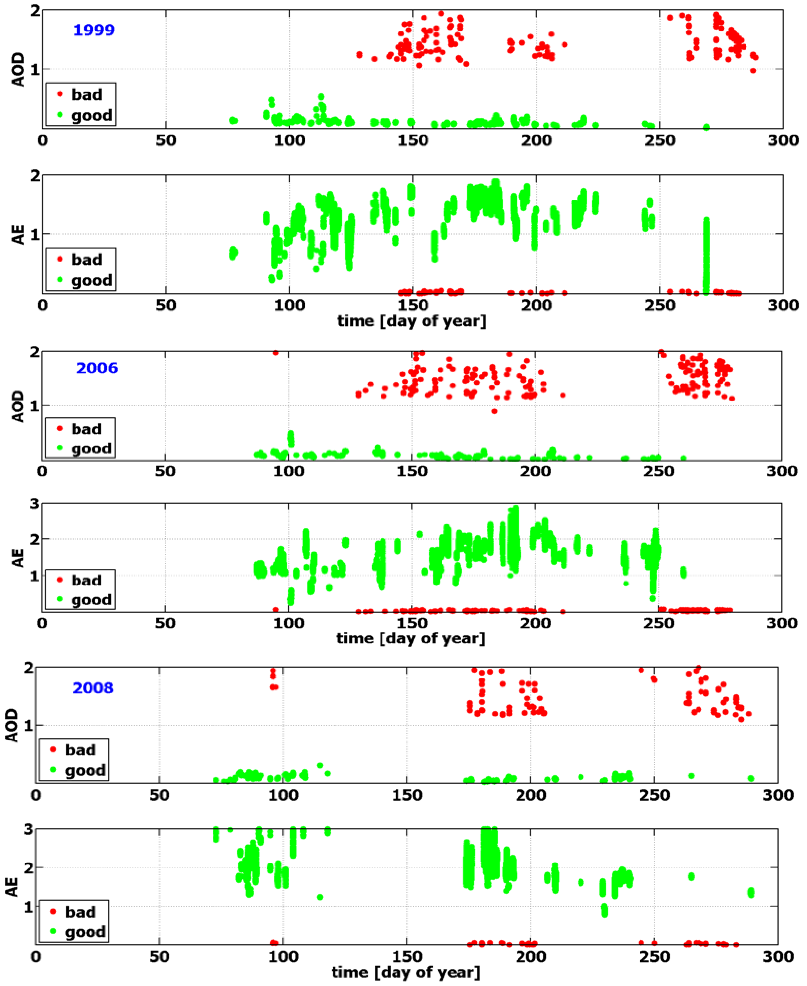
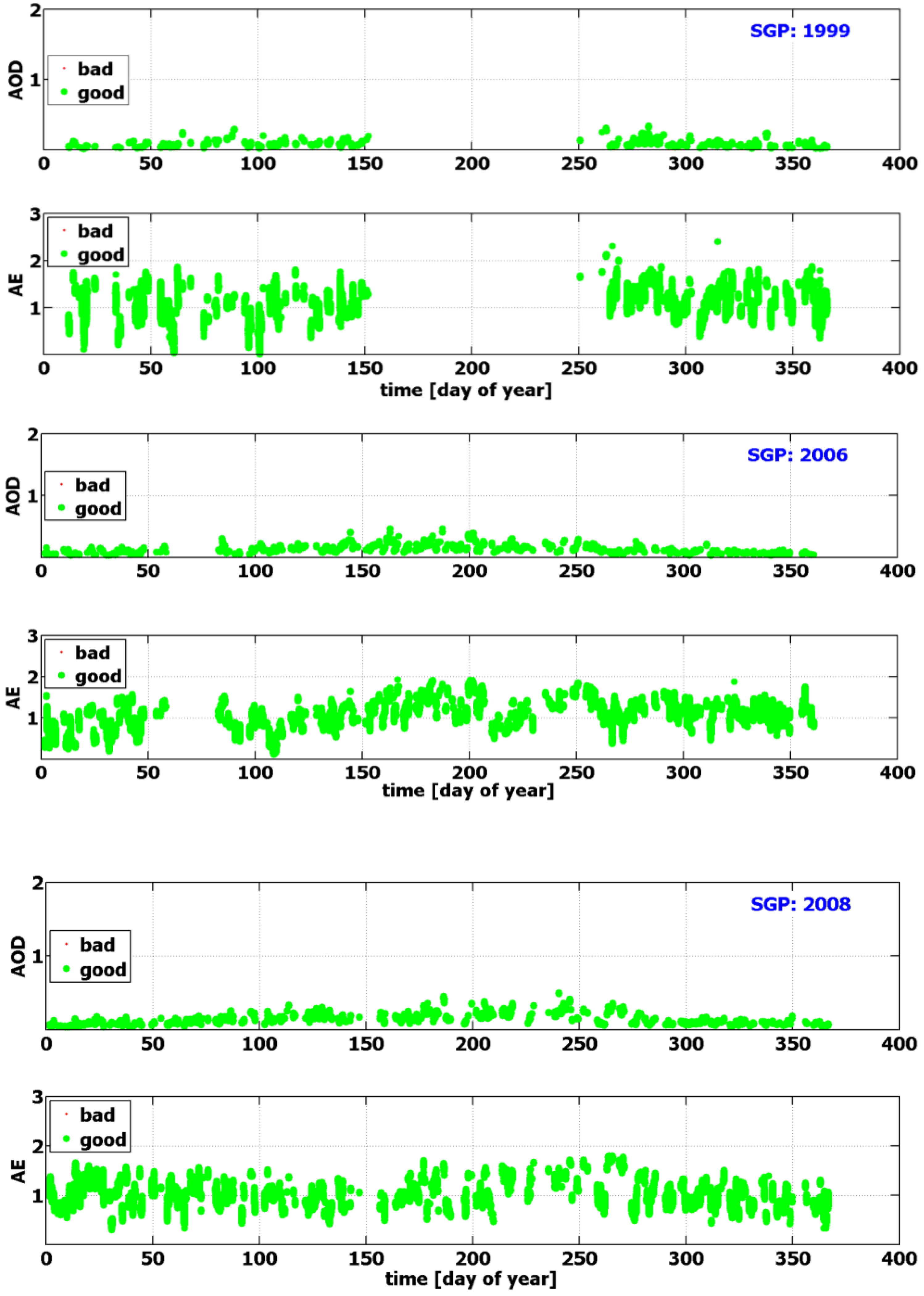
Figure 1), which depict two important features. The first is a substantial number of points with relatively large AODs (up to 2) that are likely to be cloud contaminated. The second feature is the corresponding small AE values, which indicate a significant contribution of large particles to AOD. Thus, the observed points with large AODs and small AEs are likely associated with unscreened optically thin clouds. From henceforth, points with large AODs (AOD > 1) and small AEs (AE < 0.1) will be referred as “bad” points, while points with reasonable AODs (AOD < 1) and AEs (AE > 0.1) will be defined as “good” points.
To check the occurrence of unscreened clouds, we take advantage of integrated datasets collected at the NSA sites, which include backscatter measurements from a Vaisala Ceilometer (VCEIL) and full-color sky images from a Total Sky Imager (TSI) (
http://www.arm.gov/instruments). The VCEIL is an active remote-sensing instrument for measuring vertical visibility, vertical profiles of backscatter, and cloud-base height. The TSI is essentially a vertically pointing hemispheric camera that provides time series of sky images during daylight hours every 30 s. The TSI images are commonly used for inferring several cloud macrophysical properties, such as fractional sky cover [
22,
23]. Successful application of the all-sky images and lidar measurements for an improved cloud screening has been demonstrated recently by Pérez-Ramirez
et al. [
24].
Figure 1.
Example of cloud-screened time series of Multifilter Rotating Shadowband Radiometer (MFRSR)-derived aerosol optical depths (AOD) (at 0.5 μm) and Angstrom exponent (AE) (0.415/0.870 μm) as a function of day of year at the Atmospheric Radiation Measurement (ARM) North Slope of Alaska (NSA) site in Barrow (C1 MFRSR) for three years (1999, 2006 and 2008). Cloud screening was performed using standard (or original) algorithms. Red color indicates the likely cloud-contaminated points with large AODs and small AEs (“bad” points) undetected by the existing cloud-screening algorithms. Green color represents points with reasonable AODs and AEs (“good” points).
We use the TSI and VCEIL data here only for confirming the presence of unscreened optically thin low-level clouds (cloud-base height is less than 0.5 km). It should be noted that these clouds are typically too low for reliable and quantitative detection by the onside MicroPulse Lidar [
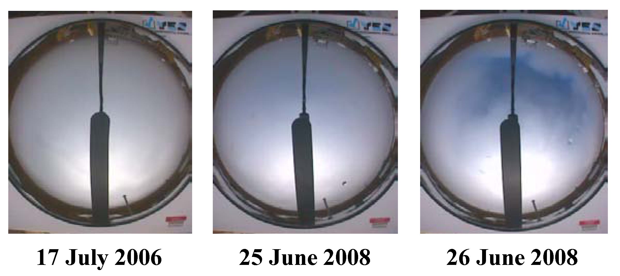
25], thus justifying our use of the VCEIL. As an illustration of our procedure, we select three days (17 July 2006, 25 June 2008, and 26 June 2008) on which large AODs and small AEs are observed (Figure 2,
Figure 3). These days are characterized by low-level optically thin clouds (note the discernible solar disk in the TSI images of
Figure 2) with little temporal inhomogeneity. For example, a single cloud layer formed on 25 June, continuing through 26 June (
Figure 3). Visual inspection of TSI images for these three days reveals temporal changes that are very small over successive 15-min time intervals. Thus, the weak cloud variability observed here can limit the performance of standard algorithms based on AOD temporal variability. The next section outlines these standard algorithms and describes the simple modification that results in an improved version of these techniques.
Figure 2.
Total Sky Imager (TSI) images for selected three days 17 July 2006, 25 June 2008, and 26 June 2008 at local noon (23 UTC). Note that even at local noon, the Sun is near the horizon.
Figure 2.
Total Sky Imager (TSI) images for selected three days 17 July 2006, 25 June 2008, and 26 June 2008 at local noon (23 UTC). Note that even at local noon, the Sun is near the horizon.
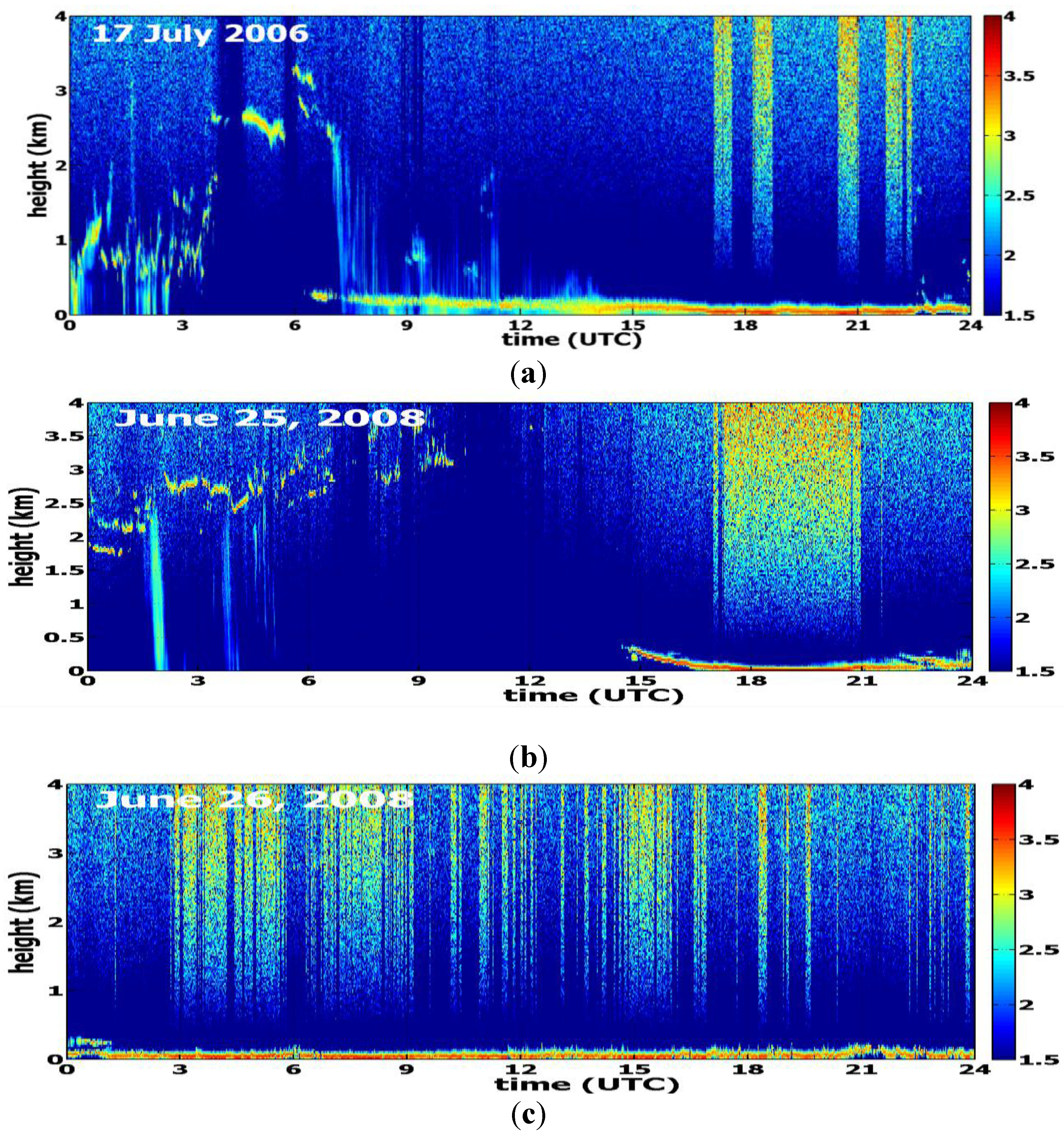
Figure 3.
Two-dimensional images of Vaisala Ceilometer (VCEIL) normalized backscatter for 17 July 2006 (
a), 25 June 2008 (
b), and 26 June 2008 (
c), corresponding to the days shown in
Figure 2. Note that a single cloud layer with long duration is located near the surface (below 0.5 km) at local noon on all three days. Increasing color wavelength (blue to yellow to red) represents increasing backscatter. Color scale defines amplitude (log of counts).
3. Improved Cloud Screening
Analysis of the observed AODs (
Figure 1) and other concurrently-obtained data (
Figure 2,
Figure 3) illustrates the occasional failure rate of the standard algorithms (
Figure 4,
Table 1). The observed failure is mainly due to two factors—atmospheric and instrumental. The atmospheric factor is attributed to the unique environment at the ARM NSA sites, including low solar zenith angle (SZA) and weak temporal variability of optically thin clouds. This factor leads to low levels of direct normal irradiance combined with relatively small temporal changes of irradiance. The instrumental factor is related to the challenging aspects of detecting irradiance signals with very small magnitudes. Small variability and low signal levels associated with the atmospheric factor interact with the discrete digital accuracy of the photodiode detectors such that the magnitude of temporal changes can be within a single count in the resolution of the instruments’ analog-to-digital converter. Thus, the digital resolution for these low signals, and even lower variability, effectively masks whatever small variability is present and leads to the false conclusion that the sky conditions are uniform and clear. Note that substantial reduction of the “bad” points during the last 4 years (2009–2012) of data (
Table 1) is mainly associated with recent MFRSR upgrades at the NSA sites.
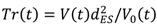
To improve algorithm performance when applied in such unique environments, we modify the original cloud-screening slightly by adding an additional threshold test based on signal level, or equivalently on magnitude of total atmospheric transmittance (Tr) for a given slant-path line of sight (as a function of time or SZA). Here the total atmospheric transmittance is defined as:
where
dES is Earth-Sun distance (in astronomical units) as a function of time (
t),
V(
t) and
V0(
t) are the measured spectrally dependent direct normal irradiance at the surface and the corresponding top-of-atmosphere irradiances (in W/m
2/nm), respectively. In comparison with the MFRSR measurements, variations of
dES change at a slow rate and can therefore be considered as time-invariant compared to drifts in MFRSR calibration factors. The top-of-atmosphere irradiance is estimated using Langley regressions, similar to Michalsky
et al. [
12].
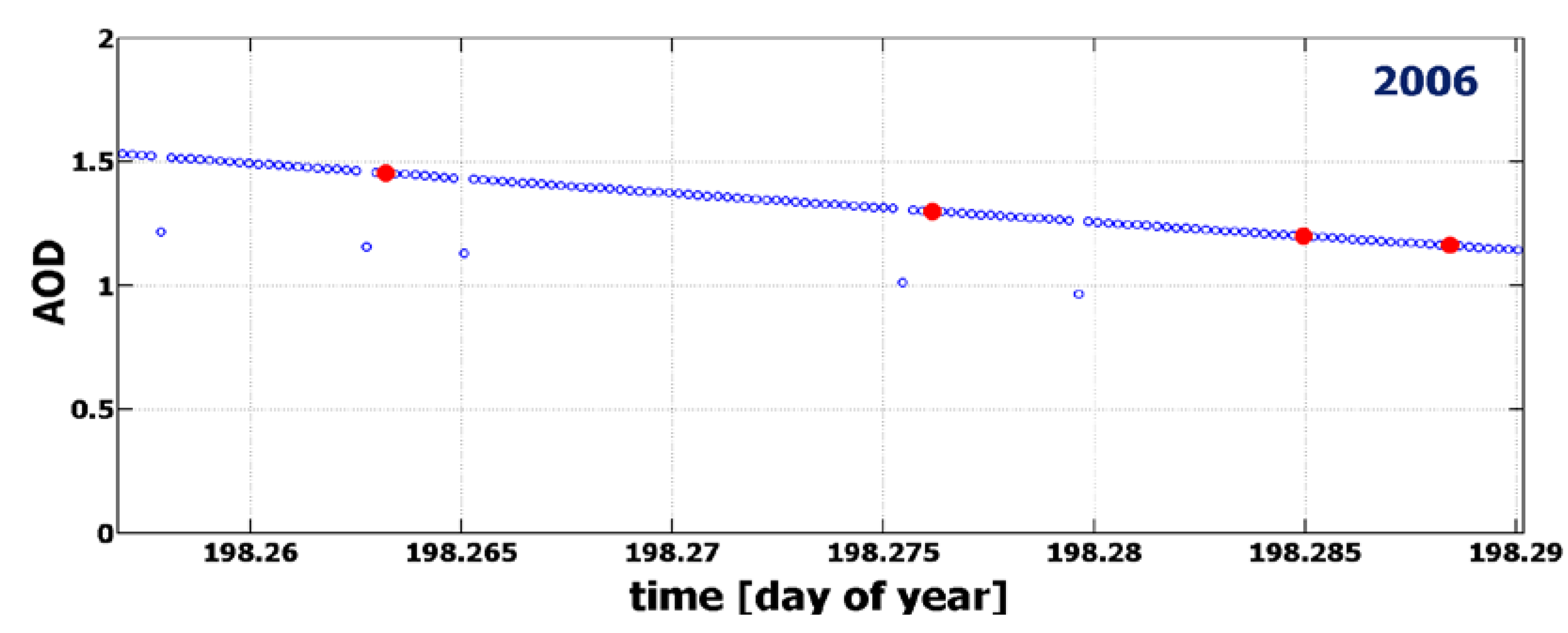
Figure 4.
Example of MFRSR-derived AOD (at 0.5 μm) as a function of day of year at the ARM NSA site in Barrow (C1 MFRSR) for 17 July 2006. Note that for this overcast day with optically thin clouds (
Figure 2,
Figure 3) there are actually no “good” points with reasonable AOD. The existing cloud screening algorithms properly identify most of points with large AOD as cloud contaminated (blue color). However, there are a few occasional exceptions when some of these points (red color) are not screened by the existing algorithms. The modified version (
Section 3) catches and removes all unscreened points (red color).
Table 1.
The total number of points with “good” and “bad” MFRSR AODs (at 0.5 μm) generated by the standard cloud-screening algorithms at the NSA Barrow site as function of year. The improved cloud-screening algorithm (
Section 2) removes all “bad” points (1999–2012).
Table 1.
The total number of points with “good” and “bad” MFRSR AODs (at 0.5 μm) generated by the standard cloud-screening algorithms at the NSA Barrow site as function of year. The improved cloud-screening algorithm (Section 2) removes all “bad” points (1999–2012).
| Year | Number of “Good” Points | Number of “Bad” Points | Fraction of “Bad” Points, % |
|---|
| 1999 | 56,939 | 181 | 0.32 |
| 2000 | 44,404 | 188 | 0.42 |
| 2001 | 42,392 | 86 | 0.20 |
| 2002 | 43,028 | 198 | 0.46 |
| 2003 | 50,998 | 172 | 0.34 |
| 2004 | 54,458 | 220 | 0.40 |
| 2005 | 55,537 | 254 | 0.46 |
| 2006 | 45,238 | 193 | 0.43 |
| 2007 | 75,102 | 140 | 0.19 |
| 2008 | 24,547 | 104 | 0.42 |
| 2009 | 14,255 | 2 | 0.01 |
| 2010 | 28,060 | 0 | 0 |
| 2011 | 15,213 | 7 | 0.05 |
| 2012 | 64,423 | 0 | 0 |
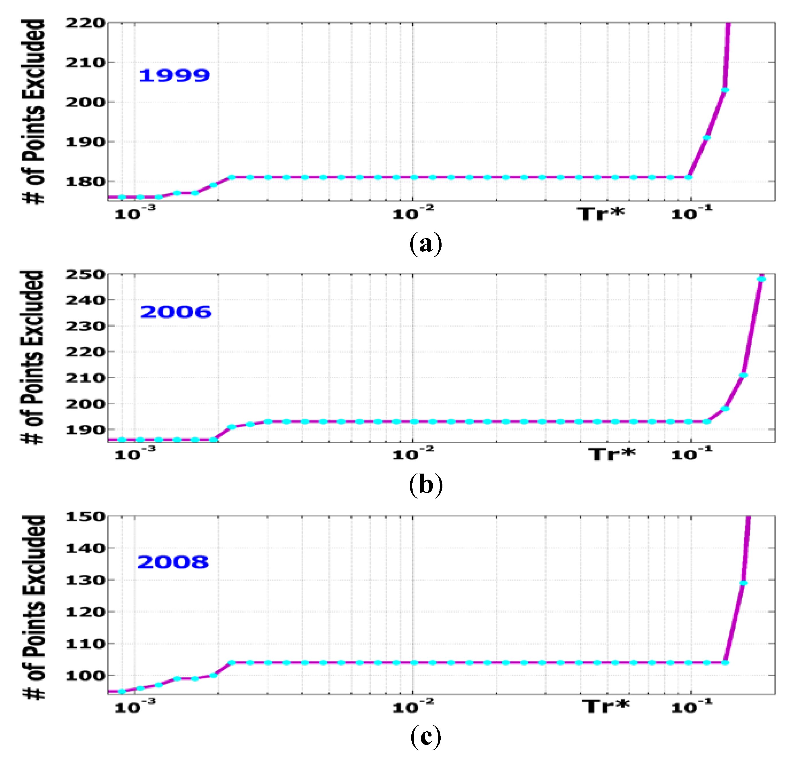
The selection of an appropriate “threshold value” (Tr*) involves two major steps: sampling a Tr* value within an expected range (0.001 to 0.1;
Figure 5), and visually checking generated plots (similar to
Figure 1) for a given Tr*. Such checking was used to confirm the anticipated reduction of “bad” points (with high AODs and low AEs), while preserving “good” points. From this empirical evaluation, we identified an optimum “threshold value” of Tr* = 0.01 for the NSA sites considered here. This value greatly reduces the number of “bad” points while retaining “good” points. The selection of Tr* is quite labor intensive, because it involves visual inspection of numerous plots. However, it seems to provide the most robust threshold value, as shown in the next section. We emphasize that this value can be site-dependent, and thus its selection should be evaluated for other locations with different types of aerosol and clouds.
In comparison with existing cloud-screening algorithms, the modified algorithm combines both the variability in the AOD/direct beam (similar to existing work) and magnitude of transmittance for a given slant-path line of sight (new). Thus, the only difference between the original and improved algorithms is an additional quality check with the fixed “threshold value” Tr*. Since this quality check involves parameters (Equation (1)) available either from measurements or standard data processing, its incorporation into existing or future cloud-screening algorithms is straightforward.
Figure 5.
Number of screened points as a function of specified transmittance threshold (Tr*) for three years: 1999 (
a), 2006 (
b) and 2008 (
c). For the selected threshold (Tr* = 0.01) the number of screened points is 181, 193 and 104 for these years, respectively. The improved version with the selected threshold (Tr* = 0.01) removes all “bad” points (
Figure 1), while keeps all “good” ones (
Figure 1). Application of an increased threshold (e.g., Tr* > 0.1 for year 1999) will result in removal of some “good” points.
4. Evaluation of Improved Cloud Screening
Success of the modified algorithm—with fixed “threshold value” Tr*—is demonstrated using a multi-year aerosol climatology collected at both the NSA and SGP sites. The objective of the evaluation is twofold: (1) illustrate the improvement of the aerosol product (AOD and AE) for the NSA sites, and (2) confirm agreement between products generated by the original and improved versions at the SGP site. The expected improvement at the high-latitude NSA sites should involve significant reduction of the cloud-contaminated points previously undetected by the original algorithms under the challenging observational conditions at these locations. Agreement at the mid-latitude SGP site would confirm that the improved version does not erroneously remove likely “good” points.
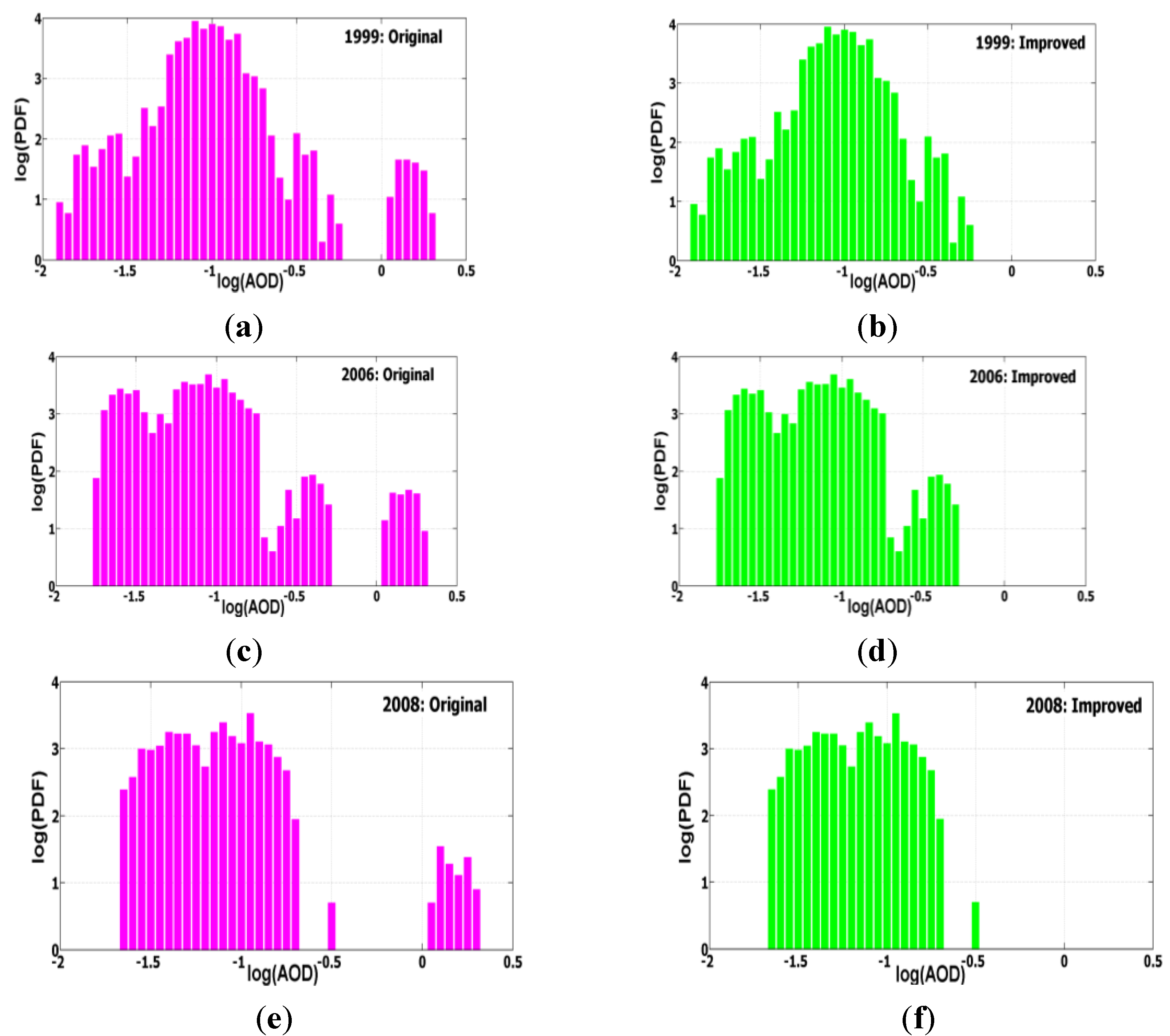
Contrasting probability density functions (PDFs) of AOD generated by the existing algorithms and the improved one are shown in
Figure 6. Consistent with
Figure 1, the original algorithms attempt to exclude all cloud-contaminated points. However, a noticeable number of them may slip through (
Figure 6; left column). Thus, a cloud-screening algorithm that is highly effective for a given location can be less robust under other conditions. The improved algorithm effectively removes only these cloud-contaminated points, while preserving “good” points (
Figure 6; right column). In a similar manner, we have confirmed the expected improvement of the MFRSR-based aerosol product for the NSA Atqasuk site, the NIMFR-based aerosol product for both the NSA sites, and for all years listed in
Table 1 (not shown).
Figure 6.
Examples of the (PDFs) of AODs (at 0.5 μm) retrieved at the ARM NSA site in Barrow, Alaska by the original (
left) and improved (
right) cloud-screening algorithms for 1999 (
a,
b), 2006 (
c,
d), and 2008 (
e,
f). These years correspond to those shown in
Figure 1. Since the relative contribution of the “bad” points to the total number of points is quite small (<0.5%;
Table 1), the log(PDF) is used. Note that the PDFs represent frequencies and they are functions of log(AOD). The PDFs generated by the original algorithms (left) include cloud-contaminated points with large AODs (log(AOD) > 0). The relative fraction of these cloud-contaminated points is 0.32, 0.43 and 0.42% for years 1999, 2006 and 2008, respectively (
Table 1).
Performance of the original cloud-screening algorithms at the SGP site is illustrated in
Figure 7 using 1999, 2006, and 2008 as representative examples. Similar results were obtained for other years. Different types of mid-latitude continental clouds have been observed at the SGP site from both the surface and space [
26,
27] and the original algorithms remove cloud-contaminated points successfully (
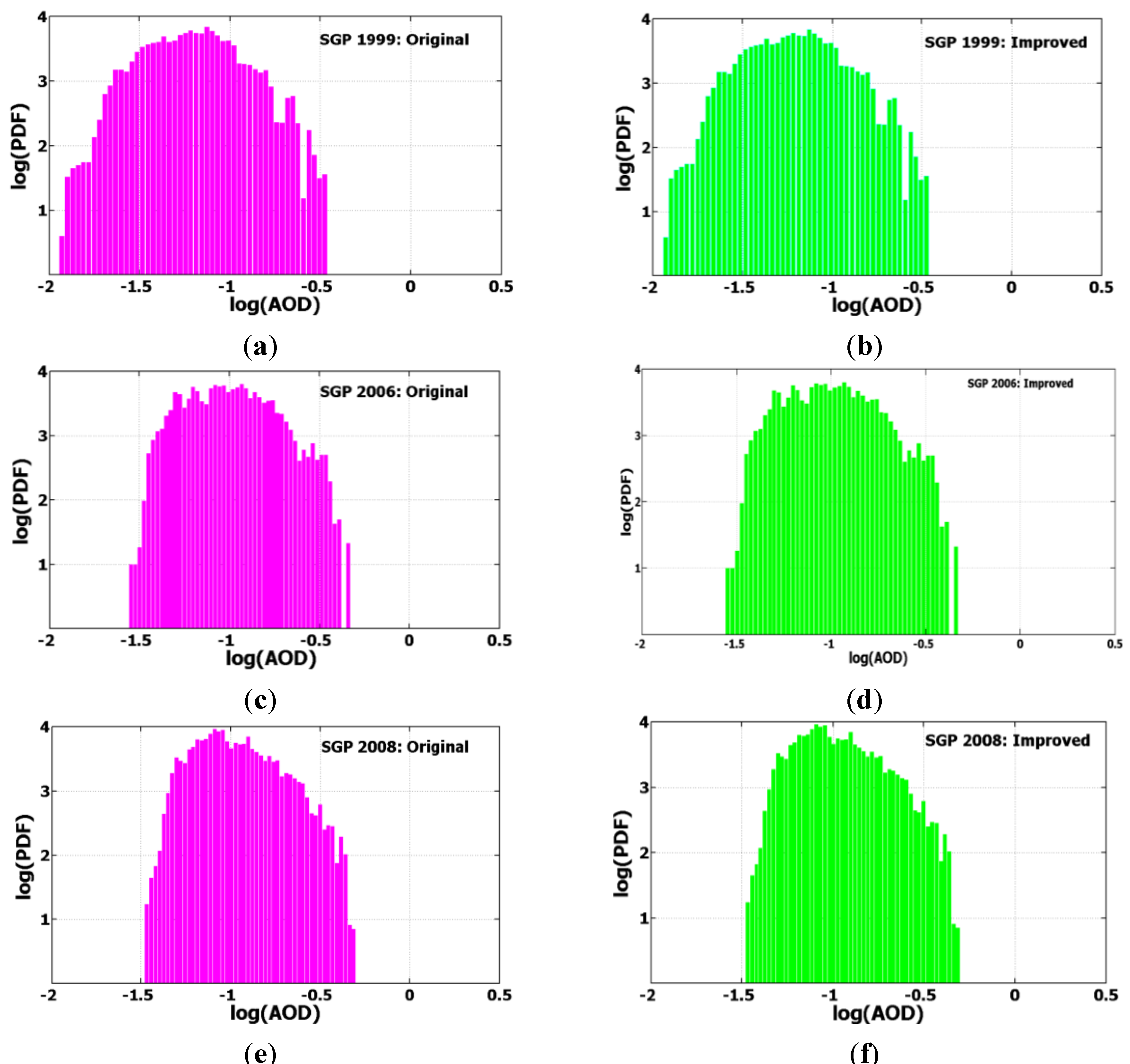
Figure 7). The agreement between PDFs of AOD generated by the original and improved cloud-screening algorithms (
Figure 8) is consistent and shows that the improved version retains the performance of the standard algorithms [
12,
16] at the SGP site, even for partly cloudy days with large variety of cloud types. It also does not erroneously remove “good” data points.
Figure 7.
As in
Figure 1, except that the time series are generated for the ARM SGP site. Note that there are no obviously cloud-contaminated or “bad” points; the standard cloud-screening algorithms are successful at this lower latitude site.
Figure 7.
As in
Figure 1, except that the time series are generated for the ARM SGP site. Note that there are no obviously cloud-contaminated or “bad” points; the standard cloud-screening algorithms are successful at this lower latitude site.
Figure 8.
Examples of the (PDFs) of AODs (at 0.5 μm) retrieved at the ARM SGP site in Barrow, Alaska by the original (
left) and improved (
right) cloud-screening algorithms for 1999 (
a,
b), 2006 (
c,
d), and 2008 (
e,
f). These years correspond to those shown in
Figure 1. Since the relative contribution of the “bad” points to the total number of points is quite small (<0.5%;
Table 1), the log(PDF) is used. Note that the PDFs represent frequencies and they are functions of log(AOD). The PDFs generated by the original algorithms (left) include cloud-contaminated points with large AODs (log(AOD) > 0). The relative fraction of these cloud-contaminated points is 0.32, 0.43 and 0.42% for years 1999, 2006 and 2008, respectively (
Table 1). Note that the improved version of cloud-screening algorithm (b,d,f) exactly reproduces the results of the original algorithm (a,c,e).
5. Discussion
At the NSA sites, the relative fraction of “bad” points is fairly low (less than 0.5%) for every year examined (
Table 1). Recall, our definition of “bad” points includes only distinct points with high AOD and low AE (
Section 2). This small fraction results in relatively small (<1%) contribution of these points into the yearly-averaged AODs. However, if the relative fraction of “bad” points is large for a given period of interest (e.g., hour, day), then they can contribute significantly to the corresponding averages. For example, there are only “bad” points for 17 July 2006 (
Figure 4) and the corresponding daily-averaged AOD for this day is large (~1.3).
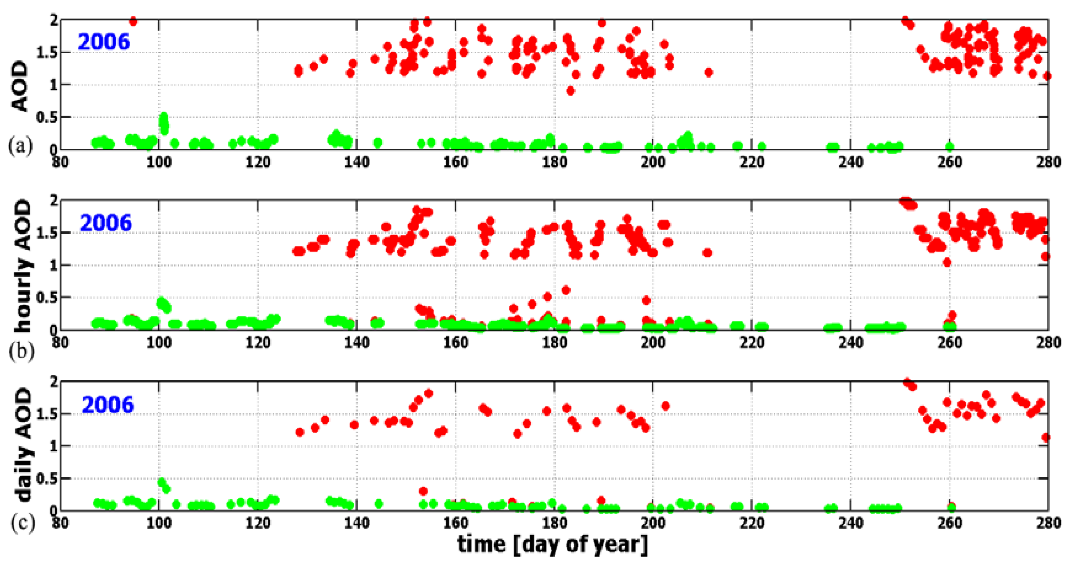
Figure 9.
Example of cloud-screened time series of MFRSR-derived AOD (at 0.5 μm) as a function of day of year at the ARM NSA site in Barrow (C1 MFRSR) for one year (2006). Similar to
Figure 1, red color indicates the cloud-contaminated “bad” points, while green color represents “good” points. The high-resolution (20-s) AODs (
a) are used for obtaining the corresponding hourly-averaged (
b) and daily-averaged (
c) AODs. The relative fraction of “bad” points is about 0.4% and 40% for the high-resolution AODs (a) and their averaged counterparts (b,c), respectively.
There are similar large daily mean values (AODs > 1) for days with large populations of “bad” points (
Figure 9). The relatively few “bad” AODs obtained from ground-based measurements with high temporal resolution (20-s) have an outsized impact on the corresponding hourly and daily averages (
Figure 9). This is because these few “bad” values that are not caught by the original cloud screen tend to occur during uniform overcast conditions when in fact no AODs
should be reported. Thus, these “bad” points dominate the corresponding averages for many individual hours or days, and therefore they are responsible for a noticeable number (~40% of time) of hourly and daily cloud-contaminated AODs (
Figure 9).
It is important to be mindful that application of the original cloud-screening algorithm at the SGP and NSA sites produces different results: numerous instances of obvious cloud contamination at the NSA sites (
Figure 1), but zero instances at the SGP site (
Figure 7). The observed differences suggest that the original cloud-screening algorithm, which is highly effective for a given regime/location (and in particular, the SGP site), can be less robust under other observational conditions. The same may be true for the improved algorithm (
Section 3). In particular, when applied to sites outside polar regions, some adjustments to the transmittance threshold (Tr*) may be necessary because of different cloud types [
7,
8] or potential impacts of desert dust or biomass burning [
28,
29,
30].
6. Summary
Multi-year (1999–2012) aerosol optical depth and Angstrom exponent (0.415/0.87 μm) collected at high-latitude Atmospheric Radiation Measurement (ARM) North Slope of Alaska (NSA) sites have been used to illustrate the occasional failure (less than 0.5% of time on an annual average) of ARM-supported cloud-screening algorithms, which, however, have exhibited stable performance at other middle-to-low latitude ARM sites. We have demonstrated that such occasional failures lead to a noticeable number (~40% of time) of hourly and daily cloud-contaminated AODs, which occurred under unique and challenging observational conditions when sun was low in the sky and optically thin clouds (the discernible solar disk in the cloudy-sky images) with small spatial inhomogeneity were observed.
The slightly modified cloud-screening algorithm described here focuses on the spectrally-resolved Multifilter Rotating Shadowband Radiometer (MFRSR) and Normal Incidence Multifilter Radiometer (NIMFR) data obtained with high temporal resolution. Similar to the original cloud-screening algorithms, the modified algorithm involves analysis of temporal variability of the derived AOD. In contrast to these algorithms, the modified algorithm additionally examines the magnitude of the slant-path line of sight transmittance and eliminates points when the observed magnitude is below a specified threshold. Additional studies are needed in order to estimate the sensitivity of this threshold to different types of aerosol and clouds, and thus to demonstrate its fidelity when applied to different sites worldwide.
The success of the modified version has been demonstrated by contrasting the aerosol product (AOD and Angstrom exponent) generated by the original and improved versions in two ways. First, a substantial improvement in the aerosol product has been shown for NSA sites via removal of cloud-contaminated AODs that were previously accepted as “good”. Second, the modified version has been shown to reproduce the aerosol product at the lower-latitude SGP site, where the standard algorithm already removes most cloud-contaminated AODs. Overall, our study suggests that our proposed modification, utilizing a transmittance threshold, can improve significantly the performance of existing and future cloud-screening algorithms based on the temporal variability of AOD time series occurring under challenging observational conditions.


