Representation of Extreme Precipitation Events Leading to Opposite Climate Change Signals over the Congo Basin

Abstract

We investigate the reasons for the opposite climate change signals in precipitation between the regional climate model REMO and its driving earth system model MPI-ESM over the greater Congo region. Three REMO simulations following three RCP scenarios (RCP 2.6, RCP 4.5 and RCP 8.5) are conducted, and it is found that the opposite signals, with REMO showing a decrease and MPI-ESM an increase in the future precipitation, diverge strongly as we move from a less extreme to a more extreme scenario. It has been shown that REMO simulates a much higher number of extreme rainfall events than MPI-ESM. This results in higher surface runoff and thus less soil infiltration, which leads to lower amounts of soil moisture in REMO. This further leads to less moisture recycling via evapotranspiration, which in turn results in less precipitation over the region. In the presence of a strong radiative forcing, the hydrological cycle becomes less intense in REMO and a downward trend in hydrological variables is observed. Contrary to this, the higher amounts of soil-moisture due to the lack of extreme rainfall events in MPI-ESM enhance the hydrological cycle. In the presence of strong radiative forcing, higher amounts of soil moisture result in increased evapotranspiration which in turn results in the higher amount of precipitation. It is concluded that the land-atmosphere coupling over the Congo region is very sensitive to the change in soil moisture amounts, which is likely to play a major role in global warming conditions. Therefore, adequate and improved representation of soil processes in climate models is essential to study the effects of climate change. However, the better representation of extreme rainfall events in REMO compared to MPI-ESM can be regarded as an added value of the model.

1. Introduction

The fourth Assessment Report (AR4; [1]) of the Intergovernmental Panel on Climate Change (IPCC) states that mean global temperatures will likely rise between 1.1 and 6.4 °C (with a best estimate of 1.8 to 4 °C) above 1990 levels by the end of this century. However, at regional level, the magnitude of the climate change signal (of different variables such as: temperature, precipitation, winds etc.) and associated extremes can be substantially different compared to the global average. Besides magnitude, the robustness in the signal plays a role of utmost importance while assessing the climate change. In this respect, the greater Congo region provides less clear picture as reported in AR4 [1], with some models projecting an increase in annual total precipitation while others a decrease resulting into an uncertain projection of precipitation. The Congo basin is predominately forested which supports livelihood of 60 million people. These forests of the Congo region are the second largest rainforests in the world, covering an area of approx. 1.7 million km². Due to their immense potential in storing carbon as well as through their impact on the regional as well as the global water cycle via local water recycling, they are supposed to have a substantial impact on the climate system.

Today, the Earth System Models (ESMs) are considered to be the most advanced numerical tools to carry out global climate simulations. ESMs are fully coupled atmosphere-ocean general circulation models (AOGCMs) with the added capability to explicitly represent biogeochemical processes that interact with the physical climate and so alter its response to forcing such as that associated with human-caused emissions of greenhouse gases [2]. The general circulation of the atmosphere, which is driven by large-scale climatic forcing, can be effectively simulated by ESMs. However, these models run at a coarser horizontal resolution (typically 150–250 km), and many regional-scale climatic processes go beyond the scope of ESMs. For this reason, the nested regional climate modeling technique was developed to downscale the ESMs results to the regional scale, and thus these models are called Regional Climate Models (RCMs). By simulating the climate at a limited model domain, the higher-resolution simulations have become computationally less expensive than ESMs. RCMs now run on a grid size between 50 to 10 km, and even down to 1 km at some instances, on time scales up to 150 years.

In the regions like Congo, soil moisture plays an important role by controlling the partitioning of the available energy into latent and sensible heat flux and conditions the amount of surface runoff. By controlling evapotranspiration, it is linking the energy, water and carbon fluxes. Seneviratne et al. [3] stated that a northward shift of climatic regimes in Europe due to climate change will result in a new transitional climate zone between dry and wet climates with strong land–atmosphere coupling in central and Eastern Europe. They specifically highlight the importance of soil-moisture–temperature feedbacks (in addition to soil-moisture–precipitation feedbacks) for future climate changes over this region. However, it has also been reported that moisture is the main driver of evapotranspiration over most parts of the Congo basin, so that a relevant coupling may be expected over this area, too [4]. A comprehensive review on soil moisture feedbacks is given by Seneviratne et al. [5].

In the simulations carried out using regional climate model REMO forced with MPI-ESM (Max Planck Institute-Earth System Model) over the African region, opposite signals of rainfall are found between the two models, although REMO is driven by the large-scale forcing from the MPI-ESM simulations. REMO and MPI-ESM show a decrease and increase in the annual rainfall respectively at the end of century, and this difference in signal becomes more obvious if we move from less extreme to more extreme scenario. Keeping in view the reported future large uncertainty of precipitation in AR4, it becomes a matter of extreme importance to find out the reasons for these opposite future precipitation signals between REMO and MPI-ESM.

In the present study, an analysis of the potential reasons causing the opposite signals between the two models is presented. The rest of the paper is structured as follows. In Section 2, a brief description of models and experimental setup is presented. Section 3 deals with the evaluation of model results whereas summary and conclusions are given in Section 4.

2. Models and Experiment Setup

As mentioned earlier, the regional climate model REMO [6] is applied to downscale global simulations of the Max Planck Institute for Meteorology-Earth System Model (MPI-ESM) over CORDEX (Coordinated Regional climate Downscaling EXperiment) African domain. Here, it may be mentioned that CORDEX is an initiative by WCRP (World Climate Research Project) to downscale CMIP5 simulation using different RCMs over different domains around the globe. There follows a description of both the models and experimental setup used for the current study.

2.1. MPI-ESM

The MPI-ESM consists of the general circulation model for the atmosphere ECHAM6 coupled to the MPI Ocean Model MPI-OM [7]. The model system is further coupled to dynamic process models for marine biogeochemistry—the Hamburg Model of Ocean Carbon Cycling HAMOCC5 [8,9] and for the land biosphere—the Jena Scheme for Biosphere-Atmosphere Coupling in Hamburg JSBACH [10,11]. Here, we use experiments conducted within the frame of the Coupled Model Intercomparison Project CMIP5 of MPI-ESM [12] in the Low Resolution LR configuration with the atmosphere in spectral truncation of T63 (~1.875° × 1.875°) and 47 vertical levels, MPI-OM with bi-polar grid at 1.5° horizontal resolution and 40 vertical levels. The main conceptual differences to the predecessor model ECHAM5/MPI-OM [13,14], which was applied in CMIP3, are the fully coupled carbon cycle and the stratosphere resolved up to 0.01 hPa.

2.2. MPI-ESM Experiments

The historical experiment of MPI-ESM was initialized in 1850 from a pre-industrial control simulation which has a total length of 1,000 years with prescribed constant natural climate forcing. Starting from three different years of the pre-industrial control run, three realizations were integrated from 1850 to 2005 under observed natural and anthropogenic forcings. The natural forcing considers variations of the Earth orbit, variability in spectral solar irradiance, stratospheric aerosols from volcanic eruptions and seasonally varying natural tropospheric aerosols. The anthropogenic forcing considers well mixed greenhouse gases (CO₂, CH₄, N₂O, CFC-11, CFC-12), ozone and anthropogenic sulphate aerosols, which are spatially and seasonally resolved. Anthropogenic land cover change is modeled in JSBACH [10] based on the New Hampshire Harmonized Land Use Protocol 3 [15] for the period 1500–2100. For more details about the climate forcings see [12]. Here, we use the first realization from 1950 to 2005 for the regional downscaling experiments.

The global climate change experiments are initialized from the end of the historical experiment and are conducted until 2100 following the Representative Concentration Pathway (RCP) scenarios developed by Moss et al. [16]. MPI- ESM was used for RCP2.6 [17], RCP4.5 [18] and RCP8.5 [18] prescribing the respective concentrations of greenhouse gas, tropospheric ozone and tropospheric aerosols, which had been modeled for each RCP, and the anthropogenic land use scenarios based on Hurtt et al. [19]. The natural forcing is the same as in the historical experiment, except for volcanic aerosols, which are set to zero. Three realizations exist for each RCP experiment. In this study, we use the first realization of each global RCP MPI-ESM experiment.

2.3. REMO

The regional climate model REMO is based on the Europamodell/Deutschlandmodell system [20]. It uses a modified version of the physical parameterization package from the general circulation model ECHAM4 [21]. A linear fourth-order horizontal diffusion scheme is applied to momentum, temperature, and humidity. The finite difference equations are solved on an Arakawa-C grid. At the lateral boundaries of the model domain, a relaxation scheme according to Davies [22] is applied, which adjusts the prognostic variables in a boundary zone of eight grid boxes calculated separately for the different compartments within a model gridbox. The vegetation-dependent land-surface parameters are taken from the LSP2 dataset [23]. In REMO, the improved Arno scheme [24] is implemented to represent the separation of rainfall and snowmelt into surface runoff and infiltration.

The REMO model has already been successfully applied over several other regions of the world (e.g., Europe: Jacob et al. [3]; South America: Silvestri et al. [25]; South Asia: Saeed et al. [26,27,28]); Africa: Haensler et al. [29,30]).

2.4. REMO Experiments

The first realization of the MPI-ESM historical experiment and of the RCP2.6, RCP4.5 and RCP8.5 experiments are downscaled with REMO to the CORDEX Africa domain. The historical experiments are downscaled for 1950 to 2005 and the RCP experiments for 2006 to 2100, respectively. The global data is prescribed at the lateral boundaries of the domain with an exponential decrease towards the inner model domain. The horizontal target resolution is 0.44° on a regular grid, the vertical atmosphere contains 27 levels on a hybrid vertical coordinate system. The time series of the observed greenhouse gas concentrations are prescribed to the regional historical simulation, the time series of the projected greenhouse gas concentrations are prescribed to the respective regional RCP experiment. Ozone and aerosols are not considered in the regional experiments, the natural climate forcing is constant. Also, anthropogenic and natural land cover is kept constant in our experiments.

3. Results

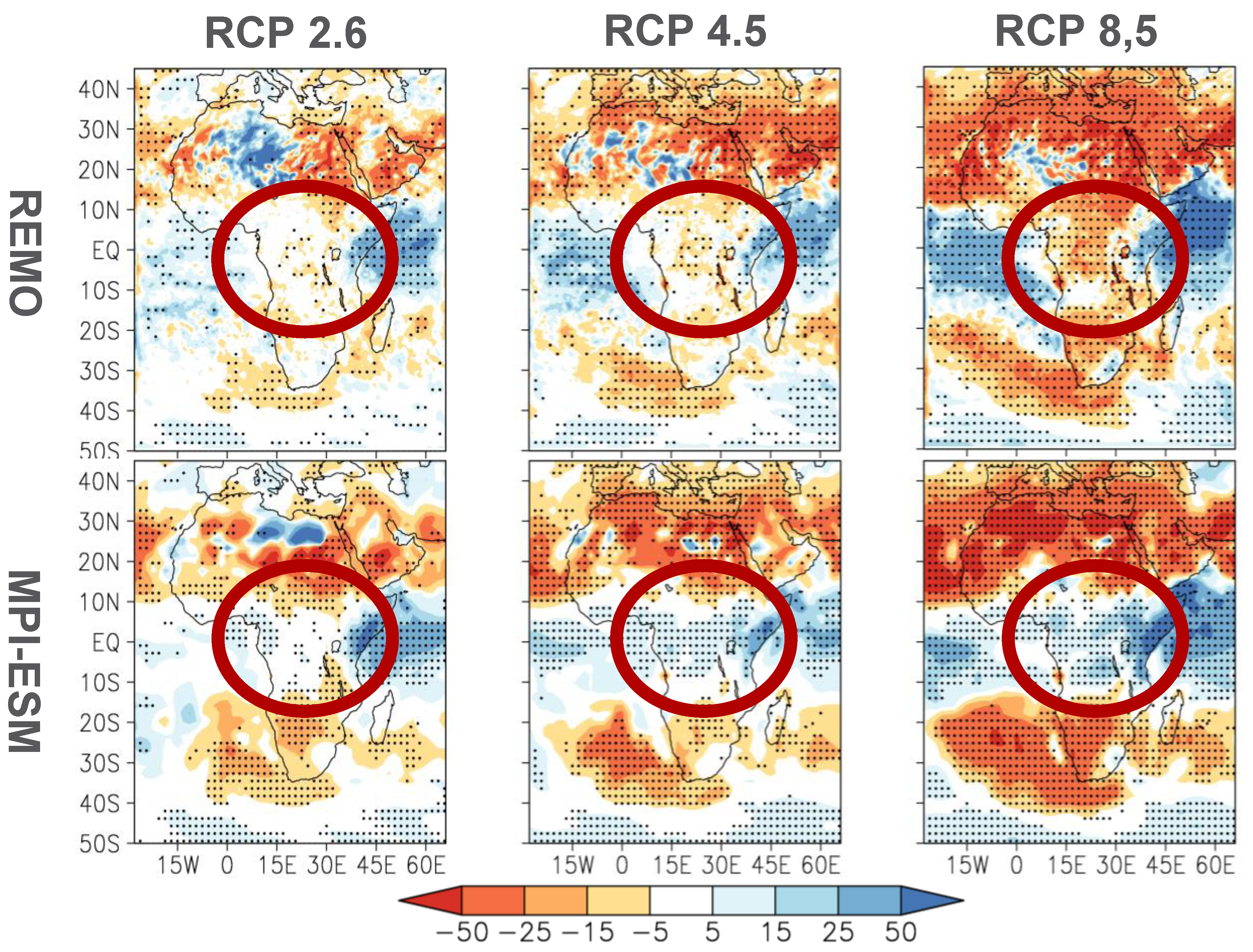
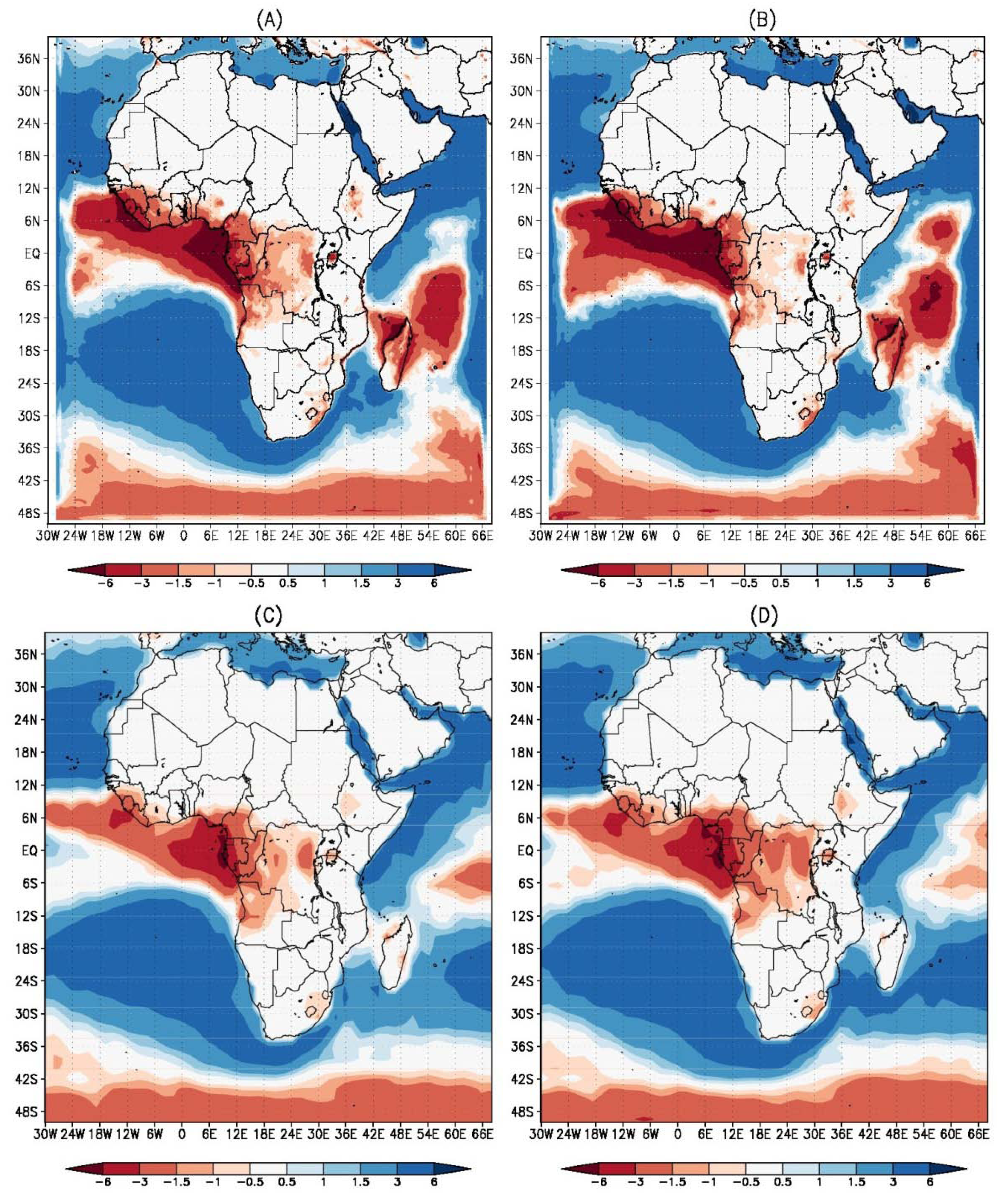
In the REMO simulation forced with MPI-ESM, statistically significant (Mann-Whitney U-test; 95th confidence interval) but opposite signals in precipitation are found in both the models towards the end of 21st century over the greater Congo region, where MPI-ESM has shown an increase and REMO a decrease (Figure 1). It can further be noticed that this difference in signals is most prominent in the scenario RCP8.5, less prominent in RCP4.5 and RCP2.6 does not show a prominent change in both the models. This behavior points to the fact that this region is sensitive to the radiative forcing which is different in the RCPs, and both the models react differently to it.

Figure 1. Projected annual mean precipitation change (%) for the 2070–2099 period with respect to the 1970-1999 period. The MPI-ESM data is interpolated on the REMO grid. Dots represent areas with statistically significant changes (95th significance level using Mann-Whitney U-test). The red circles represent the region of contradictory signal between the models.

Figure 1. Projected annual mean precipitation change (%) for the 2070–2099 period with respect to the 1970-1999 period. The MPI-ESM data is interpolated on the REMO grid. Dots represent areas with statistically significant changes (95th significance level using Mann-Whitney U-test). The red circles represent the region of contradictory signal between the models.

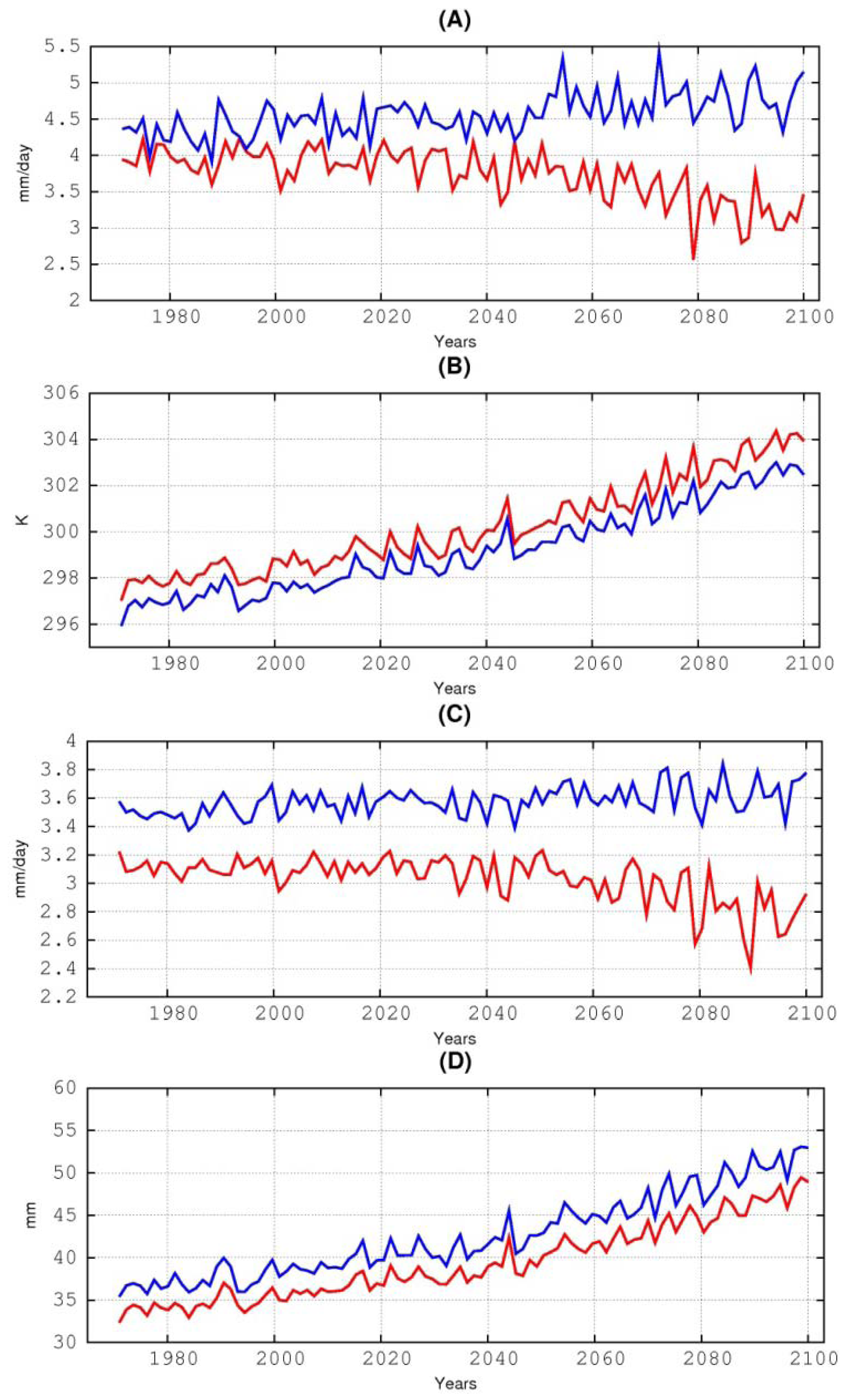
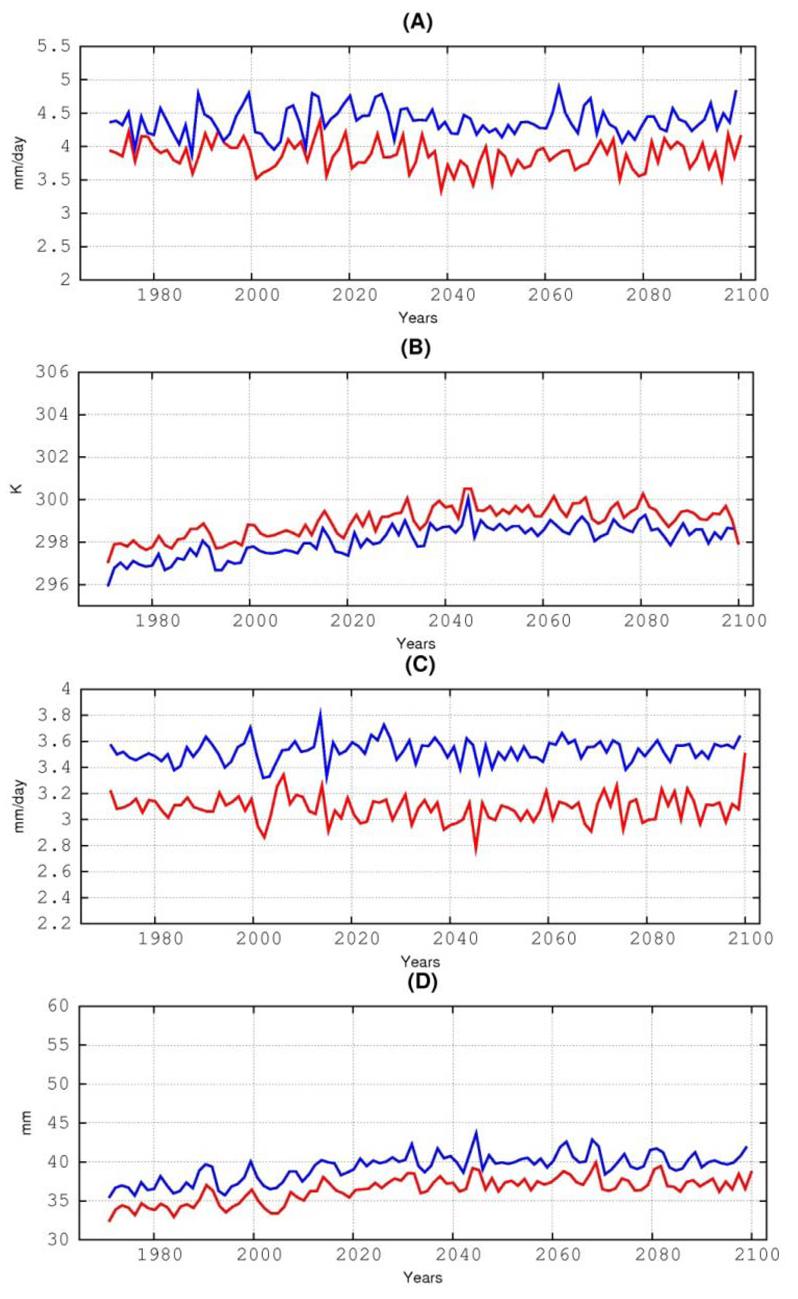
In order to find out the reason for this difference, several variables are shown in Figure 2 averaged over the region 15°E–30°E; 8°S–10°N defined as the greater Congo region. In the control period, the simulated precipitation in REMO is slightly less than MPI-ESM and the difference widens up to 2030 to 2040. However, afterwards REMO and MPI-ESM show clear decreasing and increasing trends respectively towards the end of 21st century. Further, it can be seen from Figure 2B that although REMO has simulated approximately 1°K higher 2 m-temperature than MPI-ESM, both the models show a similar increasing behavior for the 21st century. Moreover, evapotranspiration and vertically integrated water vapor (IWV) of REMO are less than for MPI-ESM throughout the control period.

Figure 2. Red (REMO) and Blue (MPI-ESM) curves represent annually averaged values over the region 15°E–30°E; 8°S–10°N for RCP 8.5. The panels show (A) Precipitation in mm/day, (B) 2m Temperature in Kelvin, (C) Evapotranspiration in mm/day and (D) Vertically integrated specific humidity in mm.

Figure 2. Red (REMO) and Blue (MPI-ESM) curves represent annually averaged values over the region 15°E–30°E; 8°S–10°N for RCP 8.5. The panels show (A) Precipitation in mm/day, (B) 2m Temperature in Kelvin, (C) Evapotranspiration in mm/day and (D) Vertically integrated specific humidity in mm.

So far, there are some obvious differences which can be seen even in the control simulation; such as higher temperatures and lower quantities of precipitation, evapotranspiration and IWV in REMO compared to MPI-ESM. Therefore, we considered the simulated atmospheric relative humidity to see whether the atmospheric demand of moisture is less in REMO than MPI-ESM, which would cause less evapotranspiration in REMO. 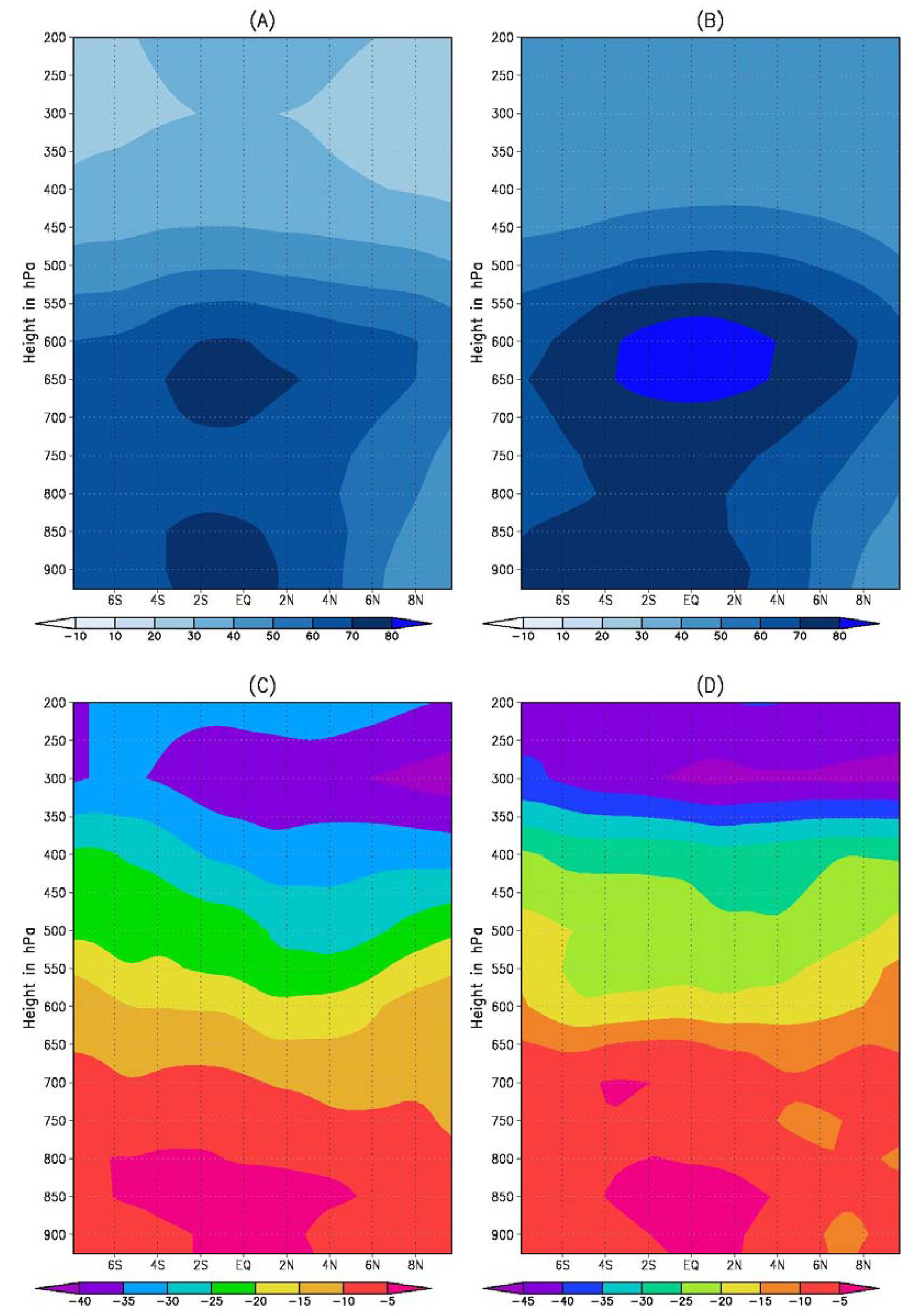Figure 3 shows the vertical and zonal distribution of relative humidity for both REMO and MPI-ESM at different pressure levels. REMO simulates smaller values of relative humidity throughout most parts of the atmosphere over the greater Congo region, which shows that there is actually a higher moisture deficit present in REMO as compared to MPI-ESM. Therefore, these results suggest that the hydrological cycle in REMO is moisture limited rather than energy limited, and soil moisture may play an important role for the behavior seen in both simulations.

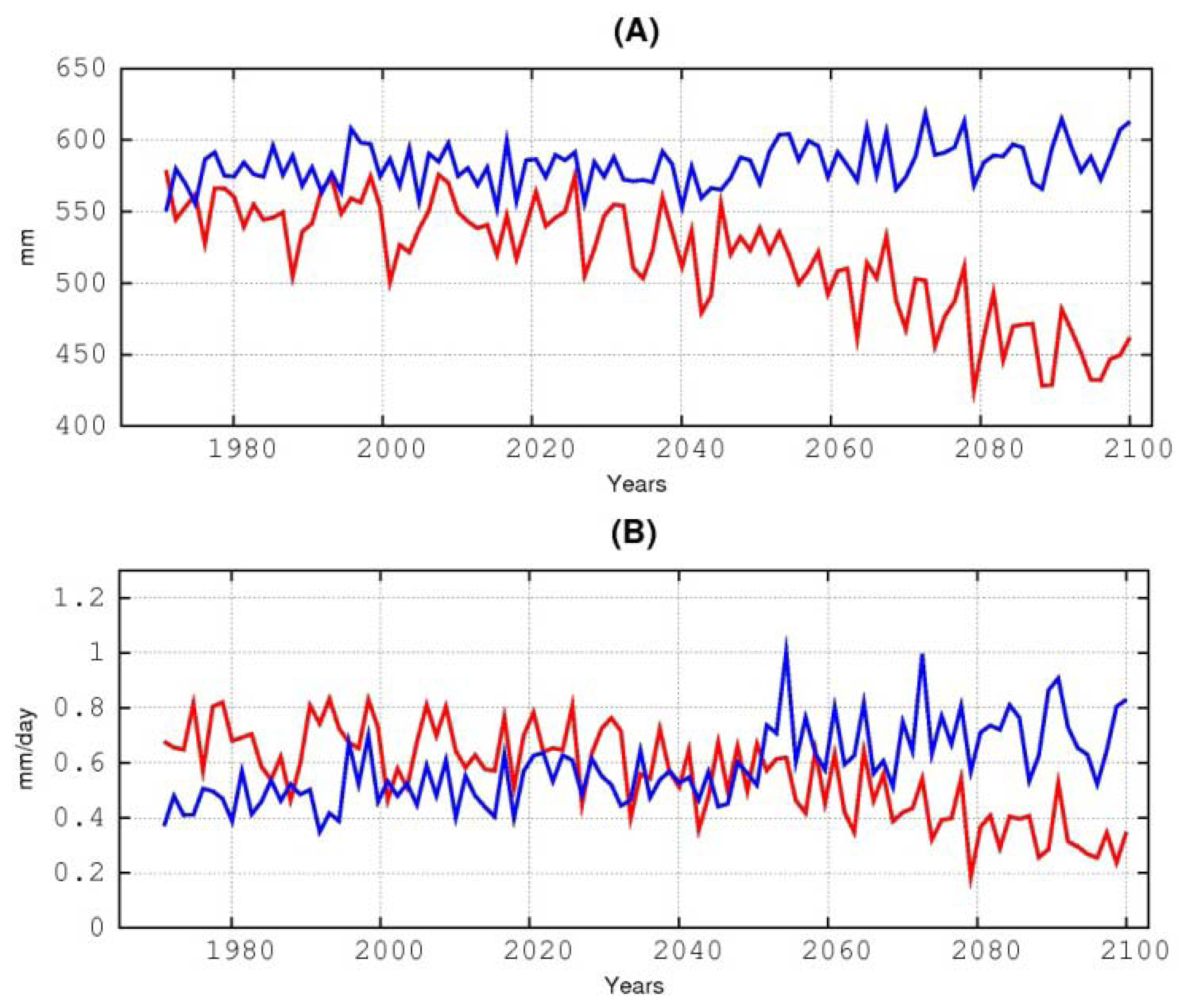
It is well established that the Congo region is one of the regions in the world where both the precipitation and temperature are sensitive to the soil moisture [31]. Soil moisture controls the partitioning of the available energy into latent and sensible heat flux, and also the amount of surface runoff. By controlling evapotranspiration, it links the energy, water and carbon fluxes [31,32]. In the control period, the soil moisture presented in Figure 4A shows that it is already less in REMO than MPI-ESM. However, a downward trend may be seen right after the start of the scenario simulation, which becomes more and more prominent toward the end of the century. In order to further explore this behavior, the simulated surface runoff is presented in Figure 4B, which shows larger values in REMO than MPI-ESM in the control period. REMO keeps on producing higher amounts of surface runoff than MPI-ESM until almost 2050, although with a gradual decreasing trend. Then it reduces further with the same trend and becomes less than that of MPI-ESM in the later half of the century. However, MPI-ESM shows the opposite behavior, with increasing soil-moisture and surface runoff after 2050.

Figure 3. North to south vertical transect of Relative Humidity (%) over the region 15°–30°E, 8S°–10°N of (A) REMO and (B) MPI-ESM, for the time period 1971–1980; and the difference between REMO and MPI-ESM for time periods (C) 1971–1980 and (D) 2071–2080.

Figure 3. North to south vertical transect of Relative Humidity (%) over the region 15°–30°E, 8S°–10°N of (A) REMO and (B) MPI-ESM, for the time period 1971–1980; and the difference between REMO and MPI-ESM for time periods (C) 1971–1980 and (D) 2071–2080.

Figure 4. Red (REMO) and Blue (MPI-ESM) curves represent annually averaged values over the region 15°E–30°E; 8°S–10°N for RCP 8.5. The panels show (A) Total soil moisture in mm and (B) Surface runoff in mm/day.

Figure 4. Red (REMO) and Blue (MPI-ESM) curves represent annually averaged values over the region 15°E–30°E; 8°S–10°N for RCP 8.5. The panels show (A) Total soil moisture in mm and (B) Surface runoff in mm/day.

Although there is a difference in the representation of hydrological processes between REMO and MPI-ESM, both models use a variant of simple bucket scheme for the representation of soil hydrology proposed by Manabe [33]. Moreover, apart from a few modifications in REMO, the scheme used for partitioning of the total amount of water available for runoff generation into surface runoff and infiltration (the so called Arno-scheme) is almost the same in both the models. In REMO the improved Arno scheme [24] is implemented to represent the separation of rainfall and snow melt into surface runoff and infiltration, which is a further development of the Arno scheme [34] used in ECHAM5. Since there is no significant involvement of snow over the Congo region, this large difference in the production of surface runoff cannot be explained by these differences in the representation of soil hydrology in both the models.

The above-mentioned discussion points towards the two possible explanations of this behavior. One cause for the higher amount of surface runoff could be the higher frequency of intense rainfall events. When the rainfall intensity exceeds the infiltration capacity of the soil, it results in the generation of surface runoff. Therefore, in order to address this issue, it becomes worthwhile to look at the performance of both the models in their representation of extreme rainfall events. Further, the more trivial reason for this opposite signal could be the difference in horizontal transport of moisture from outside the greater Congo region. These two possible reasons are dealt with in more detail in the proceeding sub-sections.

3.1. Analysis of Precipitation Extremes

In the analysis of extreme rainfall events, WATCH forcing data (WFD; [35]) has been used to define the threshold for the extreme rainfall. The value of the 95th percentile of the mean daily precipitation of wet days averaged over the greater Congo region (15°E–30°E; 8°S–10°N) for the time period (1961–1990) is defined as an extreme rainfall. Here, the wet days are defined as the days having precipitation more than 1 mm/day. Therefore, for both models, if the daily rainfall amounts become larger than this threshold (~34 mm/day), it is considered as an extreme rainfall event. Results from the extreme rainfall event analysis are presented in Table 1. From the WFD data averaged over the Congo region, the number of days with rainfall greater than or equal to the threshold is ~186 days in the 30 year period. It can be noticed from Table 1 that REMO has simulated 135.6 days of extreme rainfall, which is much closer to WFD compared to only 12.39 days of MPI-ESM during the control period. This result explains the large surface runoff and lower soil moisture values simulated by REMO compared to MPI-ESM.

Table 1. Number of extreme rainfall events for MPI-ESM and REMO for scenarios RCP2.6, RCP4.5 and RCP8.5 and for three time periods 1961–1990, 2036–2065 and 2071–2100.

	ECHAM			REMO
	1961–1990	2036–2065	2071–2100	1961–1990	2036–2065	2071–2100
RCP2.6	12.39	18.95	18.03	135.6	137.1	138.7
RCP4.5	12.39	29.57	31.6	135.6	144.6	144.4
RCP8.5	12.39	36.92	64.86	135.6	146.8	140.8

Table 1. Number of extreme rainfall events for MPI-ESM and REMO for scenarios RCP2.6, RCP4.5 and RCP8.5 and for three time periods 1961–1990, 2036–2065 and 2071–2100.

	ECHAM			REMO
	1961–1990	2036–2065	2071–2100	1961–1990	2036–2065	2071–2100
RCP2.6	12.39	18.95	18.03	135.6	137.1	138.7
RCP4.5	12.39	29.57	31.6	135.6	144.6	144.4
RCP8.5	12.39	36.92	64.86	135.6	146.8	140.8

As the simulated surface runoff is purely driven by infiltration excess, the less intense rainfall in MPI-ESM leads to more infiltration so that the soil tends to retain more moisture than REMO. In REMO due to the large number of extreme rainfall events, the rainfall intensity exceeds the infiltration rate and results in the production of more surface runoff, so that less moisture is available for infiltration into the soil. In both models, the generated runoff is removed at each model’s time-step and is no more available for evaporation and is simply lost from the model. This corresponds to the lateral transport of water where the runoff is eventually transported out of the region by the river network. Thus, it can be inferred from Figure 4B that in REMO, a substantially larger amount of water is being removed than MPI-ESM every day.

This further explains that less availability of soil moisture for evapotranspiration in REMO causes lower evapotranspiration than simulated by MPI-ESM (Figure 2C). In the control climate, however, the lower evapotranspiration in REMO does not play a major role in affecting the rainfall because it has acquired the hydrological equilibrium between land and atmosphere in such a way that even having a lower IWV, it produces consistent amount of rainfall without any downward trend. This argument is further reinforced by the results of RCP2.6 presented in Figure 5, where it can be noticed that in the absence of a strong external forcing, REMO simulates a consistent amount of rainfall as in MPI-ESM (although less than MPI-ESM) even having lower evapotranspiration and IWV throughout the 21st century.

In the case of more extreme scenario such as RCP8.5, the atmospheric demand of moisture in the atmosphere increases (Clausius-Clapeyron) and evapotranspiration keeps the similar values as in control period until 2050 in REMO (Figure 2B). However, the soil moisture starts to go down shortly after the beginning of scenario simulation (Figure 4A). Therefore, it may be inferred that REMO evapotranspiration in RCP8.5 keeps similar values until 2050 as in the control period, but at the expense of extraction of moisture from the soil. However, for the case of extreme scenario RCP8.5, the continuous loss of water as runoff due to higher number of extreme rainfall events (Table 1) as well as the increasing atmospheric moisture demand (Figure 2D), the soil-moisture reduces to the level where it remains unable to sustain the soil moisture-evapotranspiration-precipitation feedback loop. Therefore, after around 2050, the hydrological cycle in REMO becomes less intense and an obvious decline till the end of the century in all these three quantities can be seen in Figure 2. In MPI-ESM, as mentioned earlier, less surface runoff results in high infiltration and therefore higher amount of soil moisture. Under global warming conditions, the higher availability of soil moisture enhances the moisture-evapotranspiration-precipitation loop with increasing evapotranspiration which in turn, results in a higher amount of rainfall. Therefore, the retention of higher amounts of soil moisture results in an increasing of intensity of the hydrological cycle in MPI-ESM.

Another interesting behavior can also be seen from Table 1, that in the presence of adequate availability of soil moisture, MPI-ESM follow an expected behavior with an increasing number of extreme events with an increase in radiative forcing [36]. However, in REMO, because of soil moisture limiting conditions, the number of extreme rainfall events almost stagnates in the middle of century, which reduces even further in the end.

Figure 5. Red (REMO) and Blue (MPI-ESM) curves represent annually averaged values over the region 15°E–30°E; 8°S–10°N for RCP 2.6. The panels show (A) Precipitation in mm/day, (B) 2m Temperature in Kelvin, (C) Evapotranspiration in mm/day and (D) Vertically integrated specific humidity in mm.

Figure 5. Red (REMO) and Blue (MPI-ESM) curves represent annually averaged values over the region 15°E–30°E; 8°S–10°N for RCP 2.6. The panels show (A) Precipitation in mm/day, (B) 2m Temperature in Kelvin, (C) Evapotranspiration in mm/day and (D) Vertically integrated specific humidity in mm.

3.2. Moisture Convergence and Horizontal Moisture Transport

In order to assess the flow of moisture in effecting the precipitation over the Congo region, convergence is plotted in Figure 6. Convergence C of vertically integrated water vapor flux in a grid box is calculated from the water vapor conservation equation [37]:

C = ET − P − ΔS

(1)

where, ET and P are evapotranspiration and precipitation respectively, and ΔS is the change of vertically integrated specific humidity during each model output time step for REMO and MPI-ESM. Here, the positive values represent divergence and negative values shows convergence of water vapor in each grid box.

Figure 6. Simulated convergence (mm/day) (A) REMO 1971–1980; (B) REMO 2071–2080, and (C) MPI-ESM 1971–1980;(D) MPI-ESM 2071–2080. Here negative values show convergence and positive values divergence from a grid-box.

Figure 6. Simulated convergence (mm/day) (A) REMO 1971–1980; (B) REMO 2071–2080, and (C) MPI-ESM 1971–1980;(D) MPI-ESM 2071–2080. Here negative values show convergence and positive values divergence from a grid-box.

It can be seen from Figure 6A,C, that most of the regions have the same sign which includes net convergence in the west African monsoon region as well as net divergence over the southern Atlantic. However, the region north of Madagascar towards the Indian ocean which comes under the influence of South Asian winter monsoon, opposite signs are detected with REMO showing a net convergence and MPI-ESM showing a net divergence.

Over the greater Congo region, an interesting behavior is seen in Figure 6. Both the models show convergence in the control climate. However, in future, as can be seen from Figure 6B,D, REMO has shown a decreasing whereas MPI-ESM has shown a signal of increasing convergence. This difference in signal in convergence plot may be attributed to be another cause of difference in signal in precipitation between REMO and MPI-ESM. 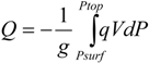Lesser amount of horizontal moisture transport in REMO in future causes reduction of precipitation and vice versa for the case of MPI-ESM. Therefore, in order to address this issue of horizontal moisture transport, we have used the following equation;

(2)

where q is specific humidity, g is gravitational acceleration constant and P is pressure. Here, V is the horizontal wind vector having the eastward and northward components. The mentioned methodology is applied on REMO and MPI-ESM data at 6 hourly data. Vertical integration is done on all the 27 vertical model levels in REMO, whereas in MPI-ESM, the integration is done after interpolating the data to the same model levels as that of REMO.

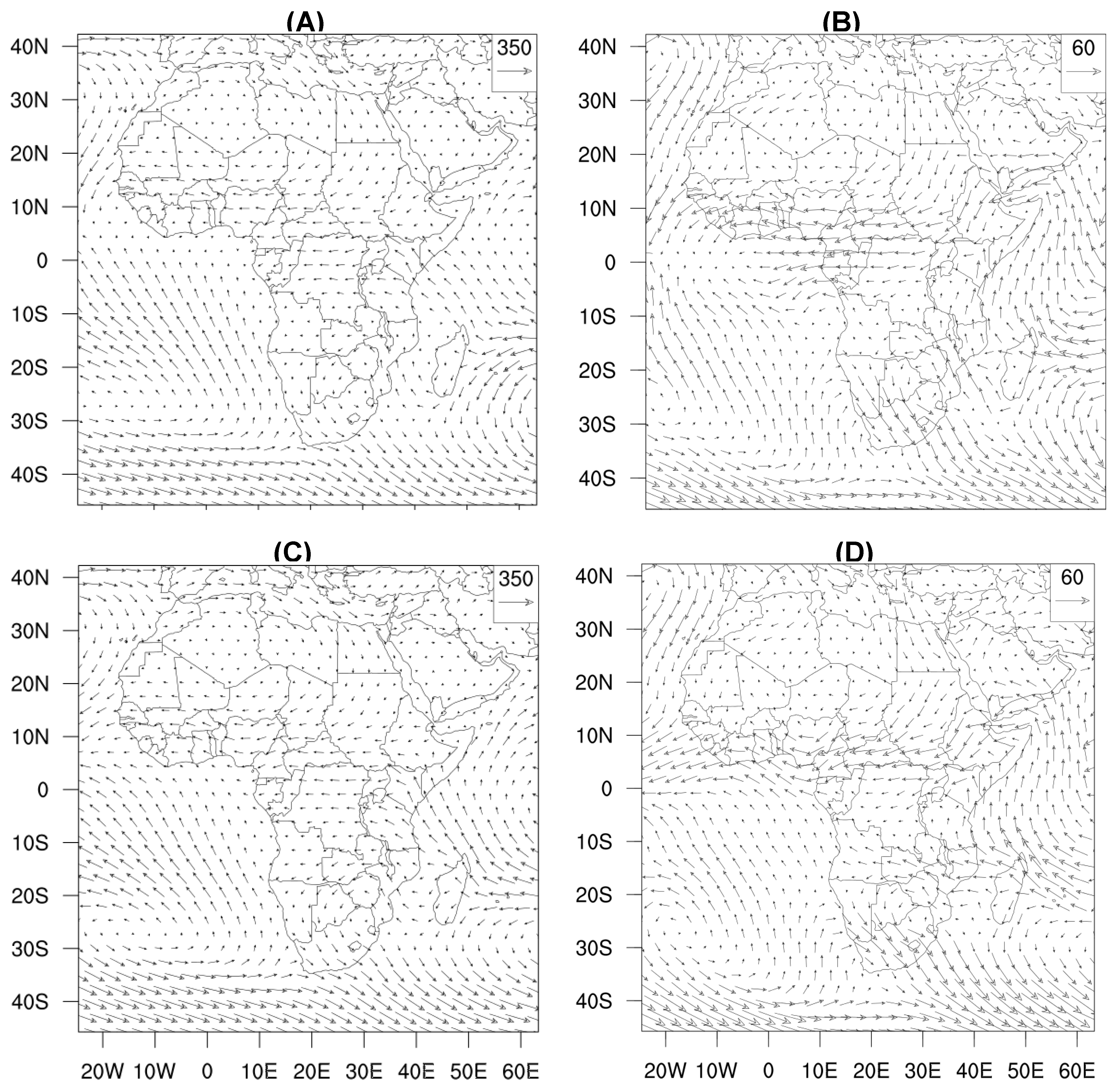
It can be seen from the Figure 7A,B, that REMO and MPI-ESM shows similar behavior of horizontal moisture transport especially towards the center of domain. Moreover, in the difference plots of Figure 7C,D, no change in direction of vectors can be found. A closer look into the plots shows the magnitude of vectors is a bit higher in REMO as compared to MPI-ESM over the Congo region. The strong divergent flow over the Congo region explains the lower future moisture convergence in Figure 6 for the case of REMO. Hence, the removal of moisture over the region might be another reason causing less precipitation in REMO as compared to MPI-ESM.

Figure 7. Simulated horizontal moisture transport (kg·m⁻¹·s⁻¹) (A) REMO 1971–1980; (B) REMO (2071–2080) minus (1971–1980), and (C) MPI-ESM 1971–1980; (D) MPI-ESM (2071–2080) minus (1971–1980).

Figure 7. Simulated horizontal moisture transport (kg·m⁻¹·s⁻¹) (A) REMO 1971–1980; (B) REMO (2071–2080) minus (1971–1980), and (C) MPI-ESM 1971–1980; (D) MPI-ESM (2071–2080) minus (1971–1980).

4. Conclusions

In this study we investigated the reasons for the opposite climate change signals of precipitation between the regional climate model REMO and the driving global climate model MPI-ESM. Three REMO simulations following three RCP scenarios (RCP 2.6, RCP 4.5 and RCP 8.5) were conducted, and it was shown that the opposite signals diverge more and more as we move from a less extreme to a more extreme scenario.

It has been found that REMO simulates lower amounts of precipitation, evapotranspiration and IWV as compared to MPI-ESM, even in the control period over the greater Congo region. Lower values of relative humidity in REMO as compared to MPI-ESM reveal that it is not the excess of moisture in the atmosphere which restricts evaporation and hence precipitation, and results in the lower values of these variables in REMO. In addition, REMO simulates lower soil moisture and a larger surface runoff than MPI-ESM. It could be shown that REMO simulates a much higher number of extreme rainfall events than MPI-ESM. This results in higher surface runoff and, thus, less amount of soil infiltration, which leads to lower amounts of soil moisture for REMO. Lower soil moisture leads to less moisture recycling to the atmosphere via evapotranspiration, which in turn results in less precipitation over the greater Congo basin. This means that the hydrological cycles becomes less intense in REMO than in MPI-ESM.

In the absence of strong radiative forcing as in the case of RCP2.6, this behavior continues throughout the 21st century with REMO simulating lower amounts of the above-mentioned hydrological variables than MPI-ESM but without any substantial trend. However, in the more extreme scenario RCP 8.5, the increasing atmospheric demand results in the increase of IWV. Initially, the evapotranspiration remains consistent on the expense of soil-moisture. However, after that, the hydrological cycle remains unable to maintain the balance. Depleting soil-moisture results in the decreasing trend of evapotranspiration which in turn results in a decreasing trend of precipitation and surface runoff, which is most clearly evident around the mid-century onwards.

In MPI-ESM for the extreme scenario RCP 8.5, the higher amounts of soil-moisture due to the lack of extreme rainfall events enhance the hydrological cycle. Due to strong radiative forcing, higher amounts of soil moisture result in increased evapotranspiration which in turn results in a higher amount of precipitation. The increasing trend is most obvious around the middle of the 21st century and afterwards.

These results show that the precipitation over the Congo region is very sensitive to the change in soil moisture, which becomes very crucial under the affect of global warming. In general, it is difficult to determine which of the two models, REMO and MPI-ESM, better represents the future climate. However, this study has shown that the simulation of extreme rainfall events, which causes different amounts of surface runoff and soil moisture in both models, plays a crucial role in causing the opposite climate change signals of precipitation between both models over the Congo region. REMO simulates the number of extreme rainfall events that is much closer to WFD than for MPI-ESM, which gives us more confidence in the REMO simulation and also shows the added value of the model. Moreover, this study points towards the need for an adequate and improved representation of soil processes in climate models, especially when regions with strong land-atmosphere coupling are considered, such as the Congo region.

Moreover, the analysis of moisture convergence shows that in the future there is a decrease over the Congo region as compared to base period for the case of REMO. However, MPI-ESM shows an increase of moisture convergence in future. This behavior is further elaborated by the results of horizontal moisture transport over the Congo region showing a slightly stronger divergent flow over Congo region in REMO as compared to MPI-ESM. Therefore, it can be inferred that, despite extreme events, the difference in signal in future moisture convergence between REMO and MPI-ESM also contributes to the difference in signal in future precipitation.

The current study is the first of its kind to report the difference in precipitation signal between an RCM driven by a GCM over Africa. The possible causes resulting in this difference, i.e., precipitation extremes and moisture transport are also discussed. However, soil moisture feedback or moisture recycling is a complex topic where it is very difficult to conclude the cause and effect. It is also difficult to conclude here which of the two causes mentioned above contributes more to the opposite precipitation signal. Moreover, using one combination of GCM-RCM may point to the issues of lack of robustness in the opposite signal of precipitation. World Climate Research Program (WCRP) has initiated a coordinated effort to downscale the CMIP5 scenarios using difference RCMS. This effort, referred to as CORDEX (Coordinated Regional climate Downscaling Experiment), currently involves more than 20 RCM groups around the world and a lot of groups are carrying out their simulations over the African domain. The availability of data from these RCMs simulation will give us deeper insight into the robustness of opposite signal of precipitation from other GCM-RCM combinations and to pin-down the possible causes leading to this signal

Besides better simulation of extreme rainfall events in REMO as well as difference in the intensity of moisture convergence in future between REMO and MPI-ESM, there may be other reasons which may contribute to the opposite signals. Differences in the clouds and radiation schemes of both models may also lead to differences in the production of precipitation. Moreover, a sudden kick in the MPI-ESM curves for surface runoff, precipitation and evapotranspiration shown in Figure 4B and Figure 2A,C respectively, is also unexplainable at the moment. This behavior may be related to the dynamic vegetation representation in MPI-ESM [10]; however, it requires further in-depth analysis. These points will be focused upon in future studies.