The Spring-Time Boundary Layer in the Central Arctic Observed during PAMARCMiP 2009

Lampert, Astrid; Maturilli, Marion; Ritter, Christoph; Hoffmann, Anne; Stock, Maria; Herber, Andreas; Birnbaum, Gerit; Neuber, Roland; Dethloff, Klaus; Orgis, Thomas; Stone, Robert; Brauner, Ralf; Kässbohrer, Johannes; Haas, Christian; Makshtas, Alexander; Sokolov, Vladimir; Liu, Peter

doi:10.3390/atmos3030320

Open AccessArticle

The Spring-Time Boundary Layer in the Central Arctic Observed during PAMARCMiP 2009

by

Astrid Lampert

^1,*,†,

Marion Maturilli

¹,

Christoph Ritter

¹,

Anne Hoffmann

¹,

Maria Stock

¹,

Andreas Herber

²,

Gerit Birnbaum

²,

Roland Neuber

¹,

Klaus Dethloff

¹,

Thomas Orgis

¹,

Robert Stone

³,

Ralf Brauner

⁴,

Johannes Kässbohrer

⁵,

Christian Haas

⁶,

Alexander Makshtas

⁷,

Vladimir Sokolov

⁷ and

Peter Liu

⁸

¹

Alfred Wegener Institute for Polar and Marine Research, Telegrafenberg A43, Potsdam 14473, Germany

²

Alfred Wegener Institute for Polar and Marine Research, Bremerhaven 27570, Germany

³

Earth System Research Laboratory, National Oceanic and Atmospheric Administration 325 Broadway, Boulder, CO 80305, USA

⁴

Jade Hochschule, Weserstr. 4, Elsfleth 26931, Germany

⁵

Fielax GmbH, Schleusenstr. 14, Bremerhaven 27568, Germany

⁶

Earth and Atmospheric Sciences and Geophysics, University of Alberta, Edmonton T6G 2E3, Canada

⁷

Arctic and Antarctic Research Institute, Bering Street 38, St. Petersburg 199397, Russia

⁸

Science and Technology Branch, Environment Canada, Downsview M3H 5T4, Canada

^*

Author to whom correspondence should be addressed.

^†

Current address: Institute of Aerospace Systems, TU Braunschweig, Hermann-Blenk-Street 23, Braunschweig 38108, Germany.

Atmosphere 2012, 3(3), 320-351; https://doi.org/10.3390/atmos3030320

Submission received: 29 March 2012 / Revised: 2 May 2012 / Accepted: 18 June 2012 / Published: 16 July 2012

Download

Browse Figures

Versions Notes

Abstract

:

The Arctic atmospheric boundary layer (AABL) in the central Arctic was characterized by dropsonde, lidar, ice thickness and airborne in situ measurements during the international Polar Airborne Measurements and Arctic Regional Climate Model Simulation Project (PAMARCMiP) in April 2009. We discuss AABL observations in the lowermost 500 m above (A) open water, (B) sea ice with many open/refrozen leads (C) sea ice with few leads, and (D) closed sea ice with a front modifying the AABL. Above water, the AABL had near-neutral stratification and contained a high water vapor concentration. Above sea ice, a low AABL top, low near-surface temperatures, strong surface-based temperature inversions and an increase of moisture with altitude were observed. AABL properties and particle concentrations were modified by a frontal system, allowing vertical mixing with the free atmosphere. Above areas with many leads, the potential temperature decreased with height in the lowest 50 m and was nearly constant above, up to an altitude of 100–200 m, indicating vertical mixing. The increase of the backscatter coefficient towards the surface was high. Above sea ice with few refrozen leads, the stably stratified boundary layer extended up to 200–300 m altitude. It was characterized by low specific humidity and a smaller increase of the backscatter coefficient towards the surface.

Keywords:

Arctic boundary layer; dropsonde; airborne lidar; sea ice thickness

1. Introduction

As a first indicator of climate change, the Arctic region has been subject to intensive investigation in the past decades and especially during the International Polar Year 2007/2008 [1]. However, atmospheric data from the central Arctic are still very limited due to its difficult access and logistical challenges of operating at the ice surface. Data are of special interest due to different feedback mechanisms, like the interaction of the Arctic atmospheric boundary layer (AABL) with surfaces dominated by open water and ice, which differ strongly in terms of skin temperature and albedo. Therefore, dropsonde observations performed by aircraft [2] and radiosonde data obtained from ship and ice surfaces (e.g., during the Surface Heat Budget of the Arctic Ocean, SHEBA campaign [3]) and the Russian North Pole Drifting stations [4] are of great value for Arctic climate research.

Arctic boundary layer processes include the exchange of momentum, heat, moisture, trace gases, and aerosol particles between the surface and the free troposphere. To date, the accurate representation of the vertical structure of the stable AABL above an ice surface still poses a serious challenge for climate modelers [5,6,7]. Model simulations of the observed summer sea-ice retreat depends on the correct simulation of the atmospheric circulation during the summer months and the sea-ice volume in the transition time from winter to spring at the beginning of the melting period [8]. Additionally atmospheric feedbacks between baroclinic cyclones and the shallow Arctic boundary layer during spring and summer conditions need a better description. Therefore targeted observations are needed to evaluate and to improve the subgrid scale parameterizations on shorter weather time scales but also on longer climate time scales in numerical weather prediction and climate models.

The thermodynamic properties of the AABL are mainly determined by solar radiative forcing, the emission of terrestrial radiation, which is determined in large part by the surface skin temperature and emissivity, turbulent heat flux, and advective processes. In the following, we summarize typical properties of the AABL above (a) open water, (b) sea ice and (c) sea ice having leads of variable width and ice thickness.

A surface dominated by open water typically entails the evolution of a convectively mixed boundary layer with an unstable layer at the bottom and a constant potential temperature profile above, strong turbulent fluxes, large moisture updrafts and the formation of cumulus clouds that cap the inversion layer [9]. Sensible and latent heat fluxes are dominant terms in the surface energy budget above the open ocean [10]. The advection of cold air masses over partly open water has a high impact on the vertical AABL structure. Due to the large heat capacity of the open water, the skin temperature is not significantly modified by colder air masses above.

Ice and snow covered surfaces or on-ice flow (air masses moving from areas above open water to ice covered areas) result in strong radiative cooling and a shallow stably stratified AABL of not more than a few hundred meters in depth that inhibits turbulent mixing. Significant diurnal thermal cycles exist over the sea ice in springtime, with typical surface-based inversions at night and mixed layers during the day in clear-sky conditions [11]. Small fluxes of sensible and latent heat are observed when data are averaged over large time or spatial scales, although they can provide significant contributions on the time scale of hours [12] and for local measurement sites [13]. A surface-based temperature inversion and moisture increase with altitude are common phenomena above sea ice for on-ice flow [14,15,16,17]. The top of the AABL depends on the distance from the ice edge, with lower values (about 150 m) farther away and higher values of a few 100 m when approaching the ice edge [18].

The AABL structure above mixed surfaces (e.g., open leads and polynyas within a sea ice covered surface) is strongly modified depending on the extent of open water [19,20], upwind/downwind conditions [14,21] and radiative forcing. In the 1980s, leads were identified as an important source of heat and moisture, where convective plumes sometimes even penetrate the free troposphere [22]. The transfer of sensible heat from small leads embedded in sea ice of very low temperatures is often more efficient than the heat transfer over completely open water [23,24].

Aerosols are observed in the Arctic in stratified layers, confined to specific altitude intervals within the boundary layer [25] or aloft depending on source regions and long-range transport [26,27]. Homogeneous mixing of aerosol up to the capping inversion is commonly observed [28]. Enhanced vertical mixing in the vicinity of open leads may be a mechanism by which soot or black carbon aerosol is deposited on the snow/ice surface [29].

During the inaugural PAMARCMiP campaign in 2009, airborne measurements of the Arctic atmosphere were performed from the POLAR-5 (Basler BT-67 aircraft, a modified DC-3) of the Alfred Wegener Institute for Polar and Marine Research (AWI). To the authors' knowledge, the concomitant measurements of aerosol optical depth (AOD), particle concentration and size distribution, black carbon concentration and sea ice thickness, combined with lidar and dropsonde measurements presented here, are the first to be performed above the remote central Arctic Ocean (at latitudes north of 80°N). Similar comprehensive sets of airborne measurements were obtained in 2008 during ISDAC [30], ARCPAC and ARCTAS [31] but without launching dropsondes and confined to lower latitudes mainly in the vicinity of Alaska. During ASCOS [32,33]/AMISA [34], dropsondes and upsondes were launched, but no lidar was operated simultaneously with the dropsondes, and only limited lidar data was collected coincident with the upsondes.

This article aims at an improved understanding of the AABL properties in the context of synoptic events and the conditions of the underlying surface. Additionally, aerosol properties (concentration and backscatter coefficient) are linked to the atmospheric structure. Based on our data availability, we apply a simple thermodynamic approach of the AABL for this study, using the vertical temperature gradient to define the AABL height, reaching from the surface to the (first) inversion top. For illustration purposes, we also determine the maximum vertical gradient of the potential temperature as an indication of the mixing layer height (transition from near-neutral / weakly stable AABL to stably stratified atmosphere, which provides an estimate of the vertical mixing height). During four flights in the central Arctic (latitude >80°N), meteorological profiles of the boundary layer were obtained by dropsondes. An overview of the dropsondes launched during these flights is given in Table 1, Table 2, Table 3, Table 4. In this article, the dropsonde profiles are analyzed with a focus on the lowermost AABL up to 500 m altitude for four different ice regimes:

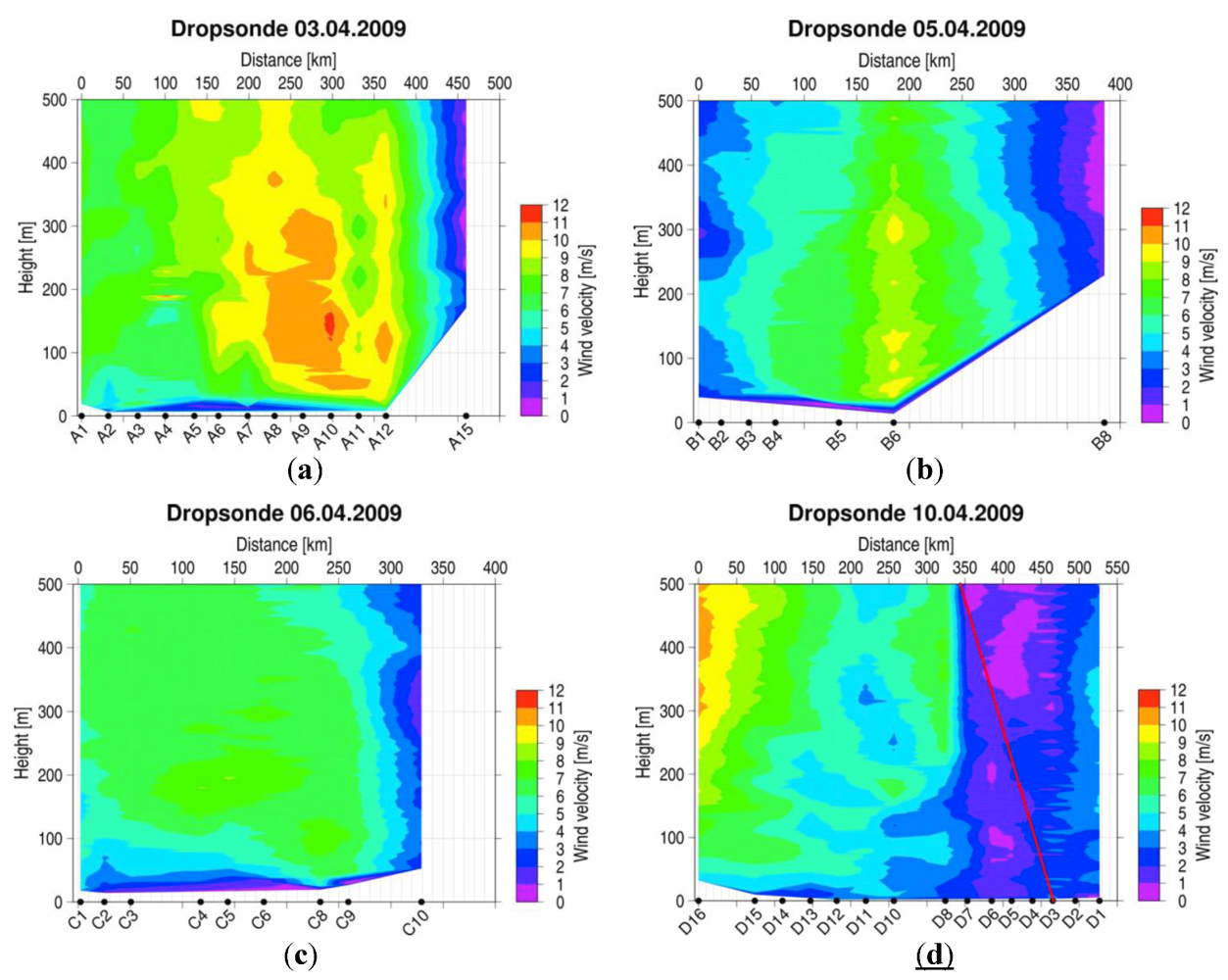
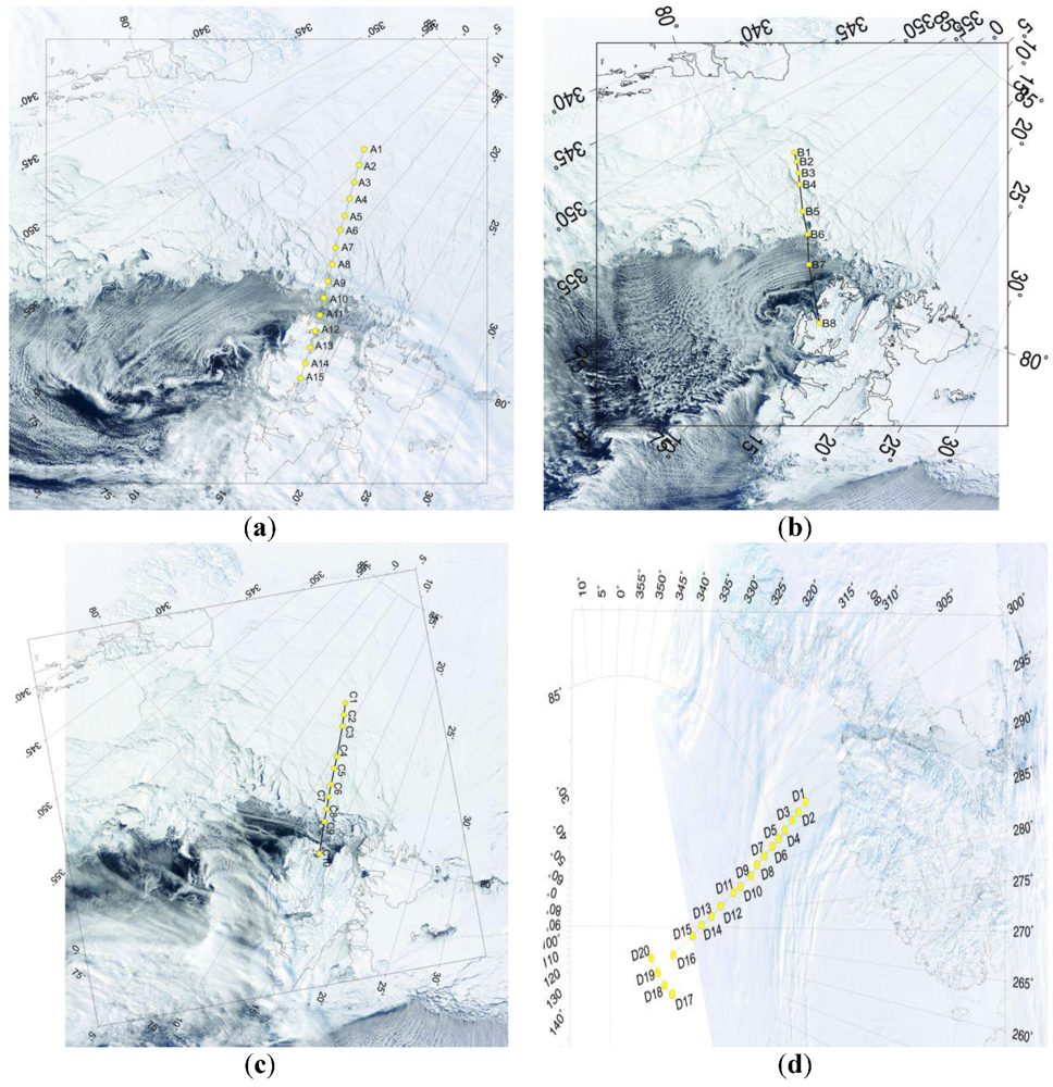
(A) the AABL above open water
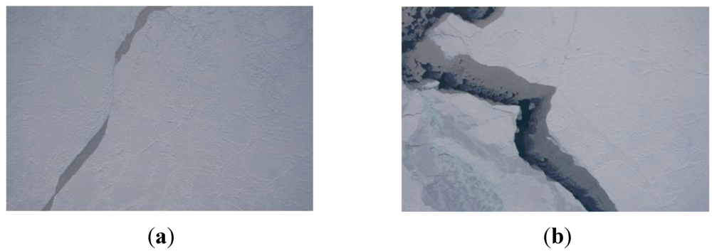
(B) the AABL above sea ice with a relatively high fraction of open / refrozen leads
(C) the AABL above sea ice with a relatively low fraction of open / refrozen leads
(D) the AABL above closed sea ice with a front passing along the flight track.

For case A, we examine dropsondes launched on a flight track north of Svalbard on 3 April 2009 (dropsondes A10–A12 in Table 1). For the cases B and C, obtained under similar synoptic conditions but with different ice regimes, we analyze dropsonde and aircraft meteorological data, and additional remote sensing data sets of sea ice thickness and profiles of the lidar backscatter coefficient. For case B (B1–B6 in Table 2), the measurement flight on 5 April 2009 covers a transect to the northwest of Svalbard back to the island between 81° and 80°N. The flight crossed the boundary between sea ice and open water. Many open and refrozen leads were embedded in the sea ice. The measurement flight of case C (C1–C7 in Table 3) is performed along a segment from Svalbard towards the north and back, between 82.5° and 80°N. Case D describes a flight to the North Pole Drifting Station (NP-36) on 10 April 2009, located at that time at 87°40'N, 117°00'W. The aircraft passed a front at about 84.5°N (close to dropsonde D3). Additionally to the dropsonde data (D1–D16 in Table 4), we analyze onboard measurements of meteorological parameters and in situ aerosol concentration.

The airborne instrumentation is described in Section 2. An overview of the meteorological situation is given in Section 3. Airborne observations are presented in Section 4 and discussed in Section 5. Finally, Section 6 provides a summary of the main results.

Table 1. Launch times and locations of the dropsonde measurements on 3 April 2009. The sondes used for case study A are highlighted in gray.

**Table 1.** Launch times and locations of the dropsonde measurements on 3 April 2009. The sondes used for case study A are highlighted in gray.
dropsonde	time (UTC)	latitude (°N)	longitude (°E)	lidar
A1	15:47	82.58	3.72	-
A2	15:53	82.33	4.72	-
A3	16:00	82.05	5.82	-
A4	16:07	81.78	6.81	-
A5	16:14	81.51	7.77	-
A6	16:20	81.27	8.46	-
A7	16:27	80.99	9.35	-
A8	16:34	80.73	10.23	-
A9	16:41	80.46	11.04	-
A10	16:48	80.18	11.79	-
A11	16:55	79.91	12.52	-
A12	17:02	79.64	13.12	-
A13	17:09	79.36	13.64	-
A14	17:17	79.09	14.16	-
A15	17:23	78.82	14.62	-

Table 2. Launch times and locations of the dropsonde measurements on 5 April 2009. The sondes used for case study B are highlighted in gray.

**Table 2.** Launch times and locations of the dropsonde measurements on 5 April 2009. The sondes used for case study B are highlighted in gray.
dropsonde	time (UTC)	latitude (°N)	longitude (°E)	lidar
B1	13:32	80.97	−3.12	available
B2	13:36	80.89	−2.02	available
B3	13:43	80.78	−0.77	available
B4	13:49	80.65	0.43	-
B5	14:05	80.33	3.09	available
B6	14:18	80.07	5.40	-
B7	14:35	79.64	7.88	-
B8	15:50	78.87	12.71	-

Table 3. Launch times and locations of the dropsonde measurements on 6 April 2009. The sondes used for case study C are highlighted in gray.

**Table 3.** Launch times and locations of the dropsonde measurements on 6 April 2009. The sondes used for case study C are highlighted in gray.
dropsonde	time (UTC)	latitude (°N)	longitude (°E)	lidar
C1	12:09	82.51	7.78	available
C2	12:15	82.30	8.49	available
C3	12:21	82.10	9.14	-
C4	12:39	81.53	10.54	available
C5	12:45	81.30	10.98	available
C6	12:53	81.01	11.57	available
C7	12:59	80.77	12.01	-
C8	13:06	80.54	12.46	-
C9	13:12	80.31	12.89	-
C10	13:31	79.71	13.98	-

Table 4. Launch times and locations of the dropsonde measurements on 10 April 2009. The sondes used for case study D are highlighted in gray.

**Table 4.** Launch times and locations of the dropsonde measurements on 10 April 2009. The sondes used for case study D are highlighted in gray.
dropsonde	time (UTC)	latitude (°N)	longitude (°E)	lidar
D1	14:17	83.98	−66.01	-
D2	14:22	84.25	−67.06	-
D3	14:27	84.50	−67.95	-
D4	14:33	84.72	−69.05	-
D5	14:38	84.95	−70.10	-
D6	14:43	85.16	−71.21	-
D7	14:48	85.43	−72.46	-
D8	14:54	85.67	−73.82	-
D9	15:00	85.88	−75.91	-
D10	15:05	86.21	−77.94	-
D11	15:11	86.52	−79.61	-
D12	15:20	86.82	−82.66	-
D13	15:27	87.08	−85.80	-
D14	15:33	87.37	−89.09	-
D15	15:40	87.62	−94.11	-
D16	15:54	88.10	−106.53	-
D17	18:22	87.78	−125.87	-
D18	18:29	88.06	−125.78	-
D19	18:36	88.36	−122.77	-
D20	18:43	88.66	−117.63	-

2. Instrumentation

2.1. Dropsonde System

The dropsonde system (Vaisala RD93 [2]) records air pressure, temperature, relative humidity, altitude, wind speed and wind direction along with GPS coordinates while descending to the ground. The vertical resolution is about 8 m. The accuracy for temperature is given by the manufacturer as 0.2 K, for pressure 0.4 hPa, for relative humidity 2%, and for horizontal wind speed 0.5 m s⁻¹. The typical time for reaching the surface from 2,000 m altitude is 3–4 min, corresponding to a horizontal distance of about 0.7 km for a characteristic average wind speed of 3 m s⁻¹. The times given for the dropsondes in the following refer to the launch. The dropsondes provide data from about 300 m below the aircraft until several meters above ground. The drop technique with fast descent of about −10 m s⁻¹ and the respective harsh landing do not allow quantifying the near-surface temperature. The lowest good data point of the dropsondes varied from profile to profile due to GPS signal quality, and was at about 20 m. Dropsondes with data not reaching below 500 m due to transmission problems were not considered in this study.

2.2. Lidar System

The lidar system AMALi (Airborne Mobile Aerosol Lidar [35]) employed onboard POLAR-5 is a backscatter lidar system operating at the wavelengths 532 nm and 355 nm. The measurements permit the derivation of depolarization at 532 nm. Developed by AWI Potsdam for airborne applications, it has a small range of incomplete overlap (250 m) from the system and is eye-safe for distances larger than 2,100 m. In this article, the backscatter profiles at 532 nm wavelength are analyzed. We use the backscatter coefficient and the backscatter ratio (BSR), defined as the ratio of total backscatter and the molecular contribution to backscattering, as this value can be compared easily to the work of other lidar groups. The lidar profiles presented here are averaged over 2.75 min, corresponding to an approximate horizontal resolution of 8.25 km at a cruising speed of about 50 m s⁻¹. The vertical resolution of the lidar profiles was 7.5 m.

2.3. Aerosol Instrumentation

Ambient aerosol was sampled via a forward facing diffuser type inlet. The aerosol sample in the inlet line was distributed to the various aerosol instruments onboard POLAR-5. The aerosol instruments included a TSI Model 7610 Condensation Nucleus (CN) counter to measure particle concentration (diameter > 14 nm), an Ultra High Sensitivity Aerosol Spectrometer (UHSAS) by Droplet Measurement Technologies (DMT) to measure aerosol size distribution and a Single Particle Soot Photometer (SP2) to measure black carbon concentration (Figure 7 in [25]).

Spectral AOD was derived using data from an 8-channel Sun photometer developed by the U.S. National Oceanic and Atmospheric Administration (NOAA) and Institute of Atmospheric Sciences and Climate‐National Research Council (ISAC-CNR), Italy. It measures spectral irradiance at central wavelengths from 368 nm to 1,050 nm. Additionally, GPS position and altitude along the flight track are recorded. The analyses methods employed are outlined in [25,36]. They include cloud-screening to minimize the influence of thin clouds as well as corrections for ozone and NO₂ attenuation. The accuracy of AOD retrievals obtained during PAMARCMiP is estimated to be within ±0.005 for wavelengths in the range 412 nm to 862 nm [25].

2.4. Ice-Thickness Sensor

Ice thickness was measured during the low-altitude flight sections, either on the outward or inward leg of all flights using a towed electromagnetic induction sensor (EM Bird [37]). By means of electromagnetic induction, the EM Bird senses the distance to the underside of the ice, which represents the interface between the resistive ice and the conductive seawater. The EM Bird’s height above the surface of the snow, ice or water is measured with a laser altimeter. The difference between both measurements corresponds to the total (ice plus snow) thickness [38]. The thickness estimates have an accuracy of ±0.1 m over level ice [38]. The ice thickness is averaged over the horizontal footprint of about 50 m. Measurements were performed at flying altitudes of approximately 100 m, with the EM bird operated 20 m above the ice surface using a 80 m long towing rope. Note that dropsondes were only launched during the high-altitude flight legs, not simultaneously with ice thickness measurements, and therefore ice thicknesses have only been used in a general way to characterize differences between different regions and ice regimes.

2.5. Meteorological Instrumentation

The instrumentation onboard POLAR-5 includes standard meteorological sensors for measuring pressure, temperature (AIMMS-20AQ sensor, Aventech Research Inc., ON, Canada), relative humidity (Humicap), and broadband hemispheric down- and upwelling shortwave and longwave radiation (Eppley pyranometers and pyrgeometers). The two Eppley pyranometers installed on Polar 5 were previously used on an aircraft of the Alfred Wegener Institute since the beginning of the 1990s (Polar 2 and Polar 4). They were regularly calibrated at the Physikalisch-Meteorologisches Observatorium Davos/World Radiation Center to determine their current sensitivity. The radiation sensors were mounted on the aircraft in a fixed position. All radiation data were corrected for their instrumental lag. The integral response time τ_s ≈ 1 s of the pyranometers was derived by spectral deconvolution of data from circling flights under cloudless conditions as performed in the 1990s with Polar 2 and 4. Eventually, the shortwave flux densities were estimated by Newton’s formula. Details are given in [39]. For clear-sky conditions, data of the upward facing pyranometer, which receives direct solar radiation, were additionally corrected for the roll and pitch angles of the aircraft to derive downwelling hemispheric radiation flux densities for horizontal exposition of the sensor (global radiation). Inversion of the Stefan-Boltzmann relation, F_lwup ~ ε σ T_s⁴ , where F_lwup is the hemispheric upwelling longwave radiation measured by the downward facing pyrgeometer, ε is the surface emissivity, σ is the Stefan-Boltzmann constant and T_s is the skin temperature, provides an estimate of skin temperature along the flight track. For simplicity, we assume the surface emissivity to be a constant 0.985 [40], although it varies slightly depending on snow and ice conditions. We furthermore neglect the contribution of reflected downwelling longwave radiation to F_lwup, because it is comparatively small. We apply the described estimation of T_s on flight legs below 120 m. At an altitude of 100 m, about 80% of the pyrgeometer signal comes from a footprint having a radius of approximately 200 m. Given the large footprint, small features, such as narrow open or refrozen leads having only slightly higher skin temperature than the ice floes cannot be resolved using this method. Hereafter, mention of skin temperature should be regarded as an effective measure due to the caveats given above, but values are considered to be a valid relative measure for purposes of analysis.

Figure 1. (a) Sea level pressure and (b) Two meter temperature data (European Centre for Medium-Range Weather Forecasts (ECMWF) analyses) averaged over the time period of the campaign, 29 March to 28 April 2009.

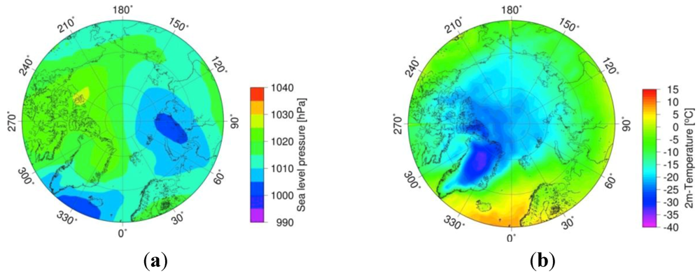
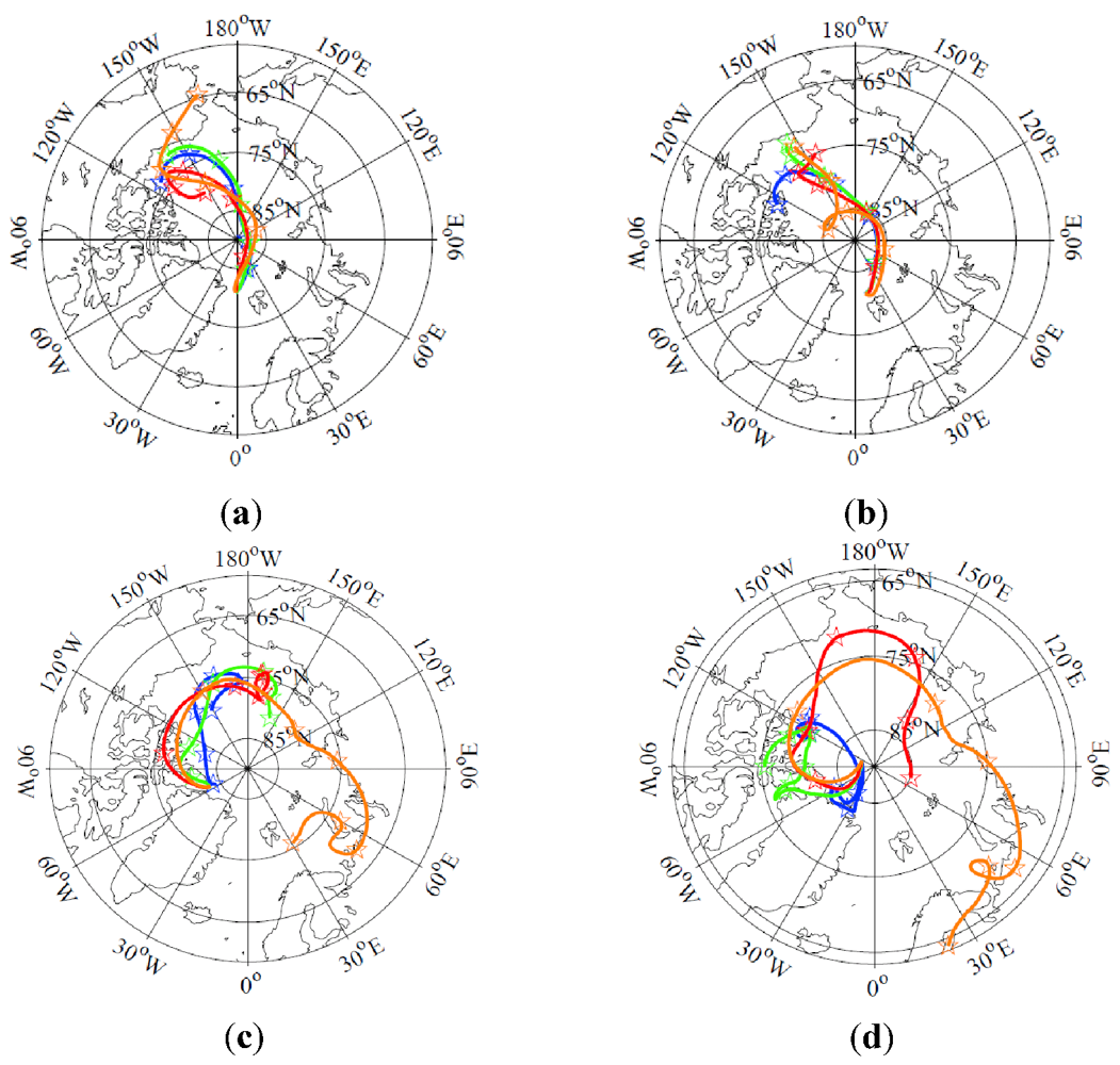
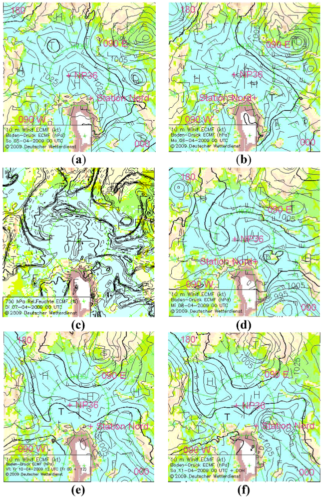
3. Meteorological Situation

The general synoptic pattern during the PAMARCMiP 2009 campaign is shown in Figure 1a. Sea level pressure data from European Centre for Medium-Range Weather Forecasts (ECMWF) analyses were averaged over the whole period of the measurement campaign. The chart of the averaged sea level pressure revealed that Svalbard was influenced on average by a low-pressure system above Siberia and a high-pressure system extending from the Canadian Arctic to Greenland. Therefore air masses passing Svalbard came from the North with 2 m temperatures below −25 °C (Figure 1b).

The flights on 3, 5 and 6 April took place under similar large-scale synoptic conditions. The synoptic pattern on 5 April (Figure 2a) featured a high-pressure system (marked with “H”) north of Greenland and a low centered east of Finland (marked with “T”). Due to this situation, clear-sky conditions were observed over the ice north of Svalbard and across to Station Nord, Greenland. Over the open water, north and west of Svalbard, stratocumulus cloud streets were present. The presence of open and refrozen leads in an otherwise closed ice pack on 5 April is evident in photographs (Figure 3) and images from the Moderate Resolution Imaging Spectroradiometer (MODIS [41], Figure 4b). On 6 April, the aircraft flew farther north, into the colder Arctic region. Here, the sea ice cover was more continuous than it was farther south (Figure 4c). On 5 and 6 April, the low-pressure system developing west of Svalbard (Figure 2(a,b)) could also be seen by the orientation of cloud streets (Figure 4(b,c)). This low got more intense by 8 April (Figure 2d) and produced heavy snowfall in that area on 7 April (Figure 2c).

Figure 2. ECMWF analyses of (a) sea level pressure 5 April 2009 at 00 UTC, (b) sea level pressure 6 April 2009 at 00 UTC (c) relative humidity at 700 hPa 7 April 2009 at 00 UTC, (d) sea level pressure 8 April 2009 at 00 UTC, (e) sea level pressure 10 April 2009 at 12 UTC, (f) sea level pressure 11 April 2009 at 00 UTC. In panel c, the areas of relative humidity exceeding 90% are marked by thick lines. Here, snowfall is possible. “T” shows low-pressure areas, “H” high-pressure areas.

Figure 3. Photographs of the surface taken on board of the POLAR-5 on 5 April 2009 while cruising at about 2,100 m altitude coincident with dropsonde B3 (a) and B5 (b). The photographs cover an area of approximately 500 m × 300 m.

For the flight to the North Pole Drifting Station (NP-36) on 10 April 2009, the weather situation was affected by a low centered at 85°N, 90°W (Figure 2e). This system was slowly moving east (Figure 2f). At its western flank, light, dry northerly winds were observed at NP-36 with few high level clouds. On the flight to NP-36, POLAR-5 passed the frontal zone at about 84.5°N. Middle and high level clouds associated with the frontal zone can be seen in the satellite image (Figure 4d), and were reported by the pilots.

Figure 4. Moderate Resolution Imaging Spectroradiometer (MODIS) high resolution images (250 m) of the sea ice conditions along the flight track on (a) 3 April, 13:15 UTC, (b) 5 April 2009, 13:05, (c) 6 April 2009, 13:45, and (d) 10 April, 19:55. The yellow dots indicate the location of the dropsonde launches (for coordinates and times see Table 1, Table 2, Table 3, Table 4). The gray lines represent the flight tracks. These images taken by the TERRA satellite were obtained from the NASA/GSFC MODIS Rapid Response web site in 250 m resolution, showing the true color spectral bands 1-4-3. The overlaid maps were drawn using the Generic Mapping Tools from [42].

4. Airborne Observations

In this section, airborne measurements of the AABL obtained with dropsonde, lidar, ice-thickness sensor and instrumentation on board of the aircraft (meteorological and in situ aerosol sensors) are presented. The typical ground speed of the aircraft is low (about 50 m s⁻¹), which provides high spatial resolution of onboard measurements at 1 Hz or higher data frequency. The launch time and location of each dropsonde is provided in Table 1, Table 2, Table 3, Table 4. We analyze four case studies measured during four different flights in the central Arctic. The focus lies on the AABL, and we discuss data of the lowermost 500 m. Three of these flights were performed from Longyearbyen, Svalbard (3, 5, 6 April 2009), and one from Alert, Canada (10 April 2009), on the way to the NP-36. Contour plots showing time-height cross sections of the profiles of temperature (Figure 5), potential temperature (Figure 6), water vapor mixing ratio (Figure 7), wind direction (Figure 8) and wind speed (Figure 9) for the discussed days are presented. They are analyzed and interpreted in Section 5. In the following, potential temperature rather than virtual potential temperature is used in order to avoid uncertainties associated with humidity measurements [43].

Figure 5. Time-height cross sections of dropsonde temperature observed along the flight legs on 3 (a), 5 (b), 6 (c), and 10 (d) April 2009. The x-axes show the location of the dropsondes (in north-south direction from left to right) used for the plots, and the distance from the northernmost dropsonde. When data are missing, parts of the panels are left white. Dropsondes, which did not deliver data below 500 m altitude, are left out. The black line with red dots in panel d shows the strongest horizontal temperature gradient for all altitudes, indicating the front. A visual approximation of the front is given by the red line, which is also used in Figure 6d, Figure 7d, Figure 8d, Figure 9d. Dropsondes A10–A12 and C9 were launched above open water.

Case A represents measurements obtained on 3 April 2009 on a low altitude flight from Longyearbyen towards the north-west, and a similar path back at 2,500 m altitude. On the way back, 15 dropsondes were launched (Figure 4a). The flight path crossed the sea ice boarder. Case A analyzes dropsondes A10 to A12, which probed the atmosphere above open water. For two cases (B and C), concomitant dropsonde and lidar measurements are presented. The two transects were flown from Longyearbyen airport out in a northerly direction and returned. The flight on 5 April (case B) was more to a northwest direction, towards Fram Strait, while the flight on 6 April (case C) was more towards the north. Therefore, different ice conditions were observed on successive days. In cases B and C, the flight altitude along the outbound leg was low (<100 m) in order to enable measurements of sea ice thickness using the EM Bird. This also allowed the study of columnar AOD as derived from Sun photometry [25]. On the return leg, the flight altitude was nominally at 2,200 m in order to study the boundary layer with the lidar and dropsonde instrumentation (dropsondes B1–B6, C1–C7). Four and five dropsonde profiles of meteorological parameters with concomitant down-viewing lidar profiles were evaluated for case B (B1–B3, B5) and case C (C1–C2, C4–C6), respectively. Case D represents measurements in the central core of the Arctic Ocean (Figure 4d). This unique data set includes dropsonde measurements and in situ aerosol concentrations. Due to technical problems, no lidar data are available for this flight.

The data were all obtained during the local daytime; however, some were sampled in the late morning (case D), near local noon (case C) and in the afternoon (cases A and B), which may have affected atmospheric stability characteristics.

Figure 6. Potential temperature as retrieved from dropsonde measurements on 3 (a), 5 (b), 6 (c) and 10 April (d) 2009. Dropsondes, which did not deliver data below 500 m altitude, are left out. The red dots in panels a, b, and c show the altitude of the strongest vertical gradient of potential temperature, which is used here as an indicator of the AABL height. The red line in panel d indicates the location of the front determined from the strongest horizontal temperature gradient.

Figure 7. Water vapor mixing ratio as retrieved from dropsonde measurements on 3 (a), 5 (b), 6 (c) and 10 April (d) 2009. The red line in panel d indicates the location of the front determined from the strongest horizontal temperature gradient.

Figure 8. Dropsonde measurements of wind direction on 3 (a), 5 (b), 6 (c) and 10 April (d) 2009. The red line in panel d indicates the location of the front determined from the strongest horizontal temperature gradient.

Figure 9. Dropsonde measurements of wind speed on 3 (a), 5 (b), 6 (c) and 10 April (d) 2009. The red line in panel d indicates the location of the front determined from the strongest horizontal temperature gradient.

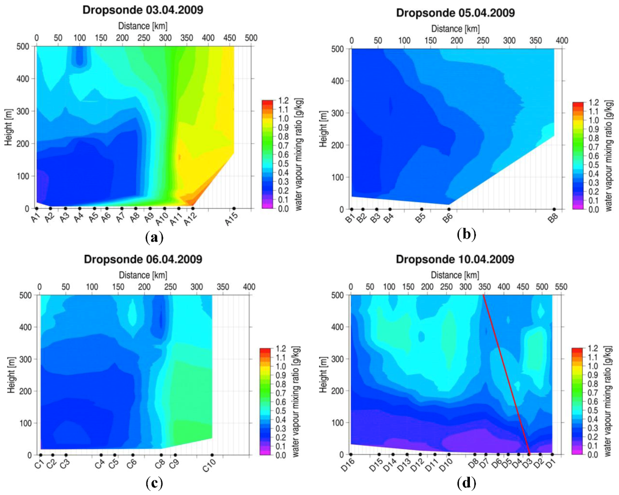
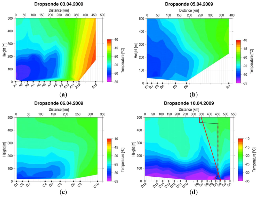
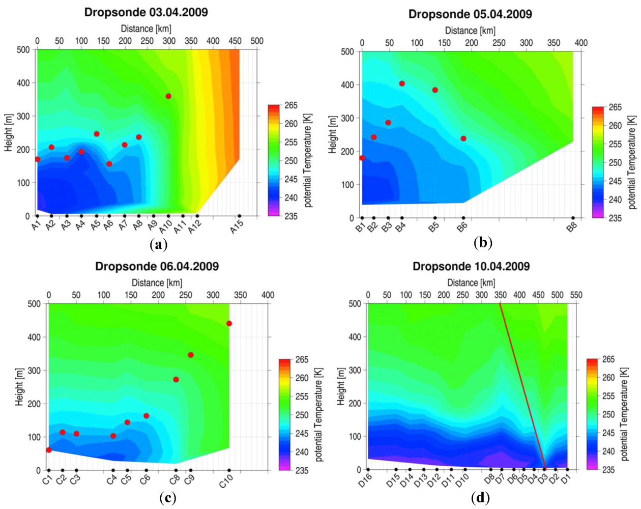
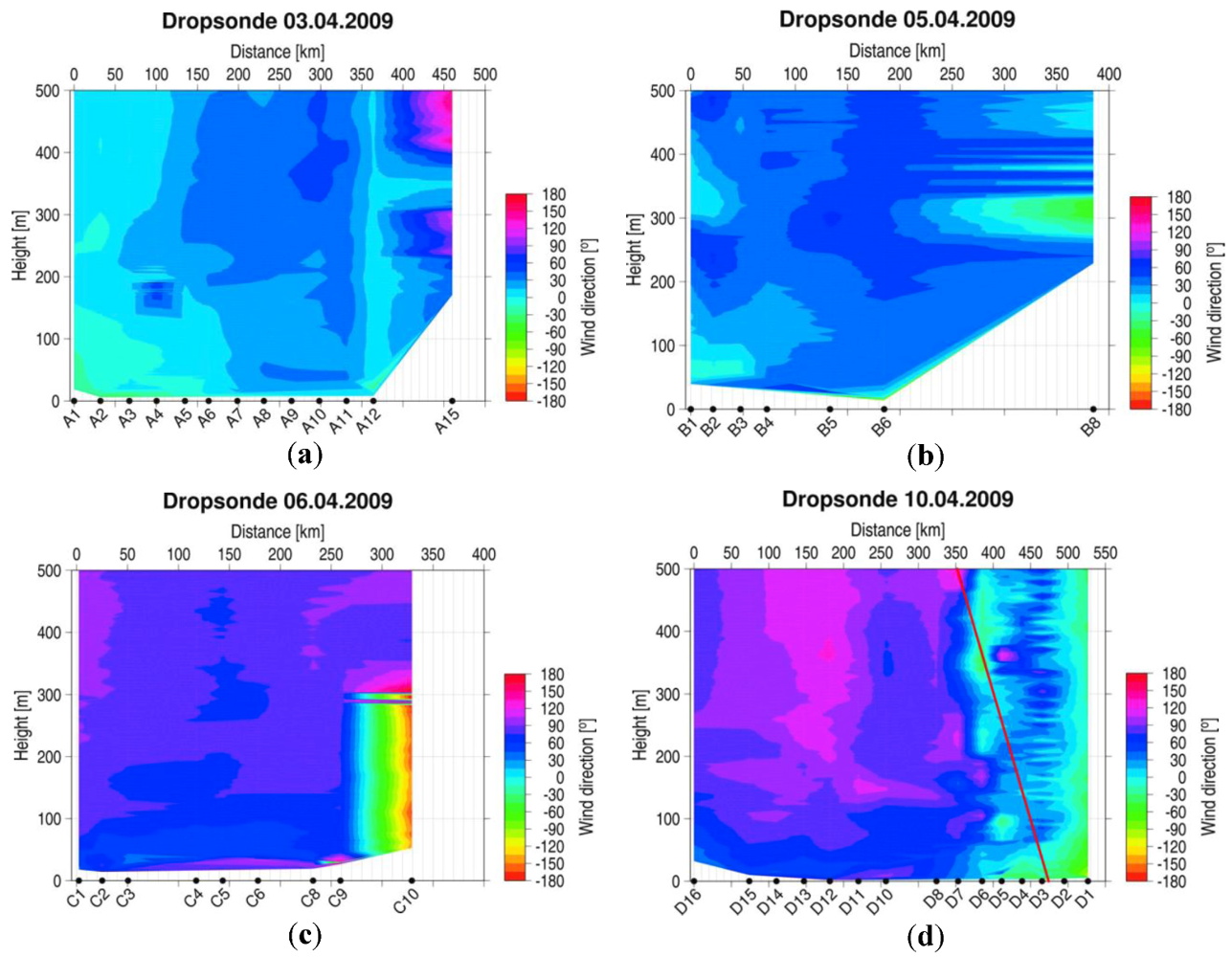
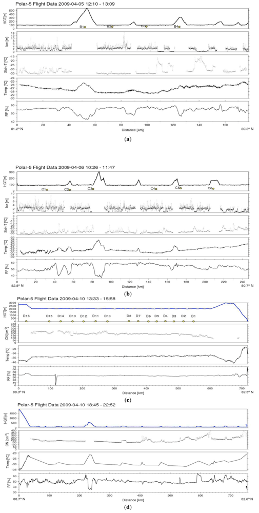
4.1. CASE A: The AABL above Open Water

As illustrative examples of the AABL above open water, we use dropsondes A10 and A11, as well as dropsonde A12, which was launched near shore Svalbard, but was strongly influenced by the open water due to northerly wind direction. Dropsonde A10 was launched about 15 km, A11 about 48 km, and A12 about 80 km from the sea ice edge (Figure 4a). The temperature profiles obtained above open water on 3 April 2009 (dropsondes A10–A12) differ clearly from profiles measured above sea ice. When descending over open water, dropsondes showed relatively warm near-surface temperatures and no surface-based temperature inversion (Figure 5a). The potential temperature was almost constant with only slight a decrease with height in the lowest 500 m (Figure 6a), implying a near-neutral/weakly unstable stratified atmosphere. In the lowest 50 m, the potential temperature decreased, which indicates turbulent mixing and vertical transport of heat and water vapor. The strongest gradient of potential temperature (red dots in Figure 6a) exceeded 300 m for dropsonde A10 and even 500 m altitude for dropsondes A11 and A12. The water vapor content was strongly enhanced with a water vapor mixing ratio exceeding the value of 1 g kg⁻¹ (Figure 7a).

Above the layer of constant potential temperature, a temperature inversion was present. The top of the temperature inversion, defined as the altitude where the temperature starts to decrease with altitude, varied between 600 m and 800 m near the sea ice edge above the open water surface (not shown).

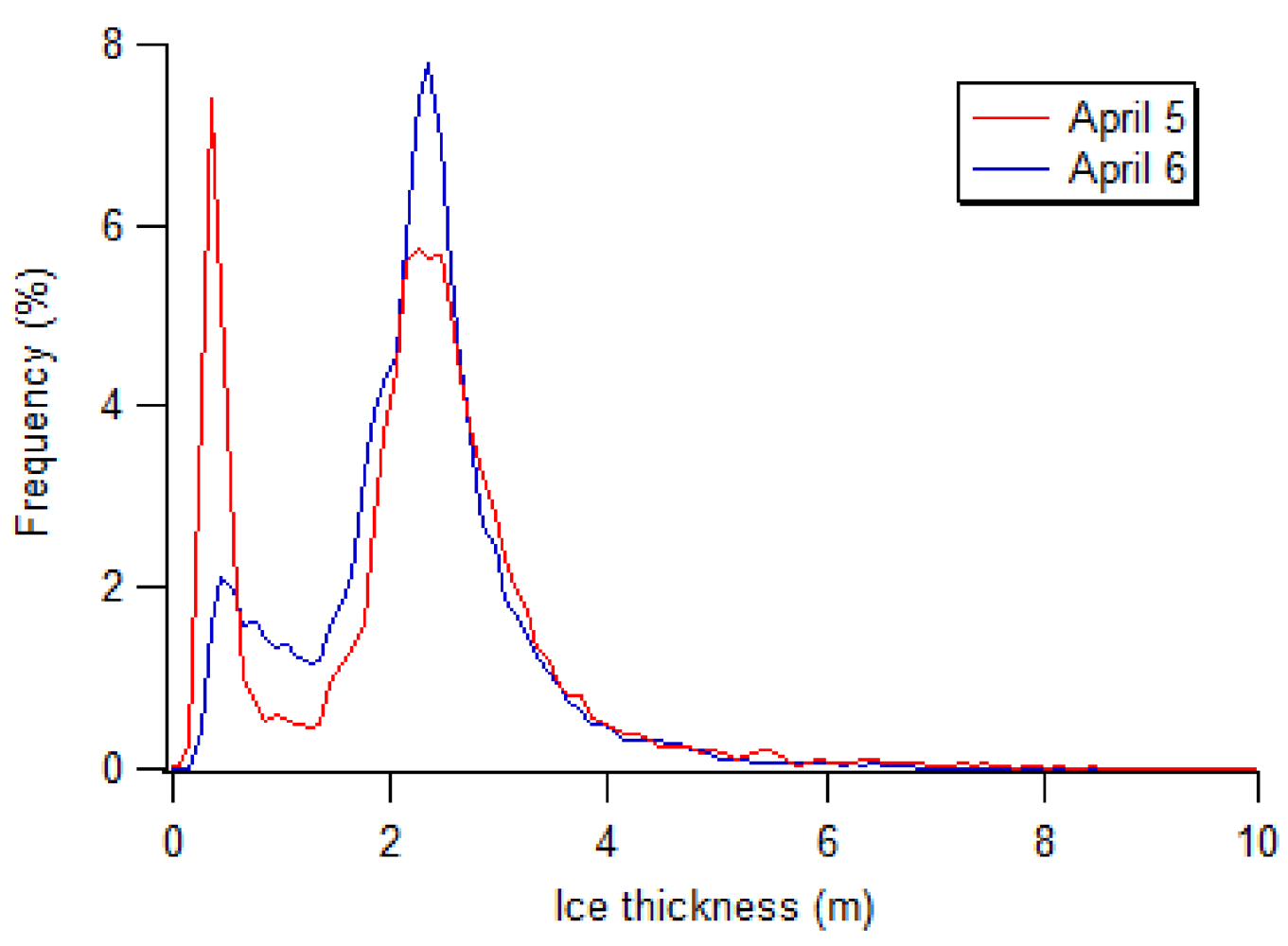
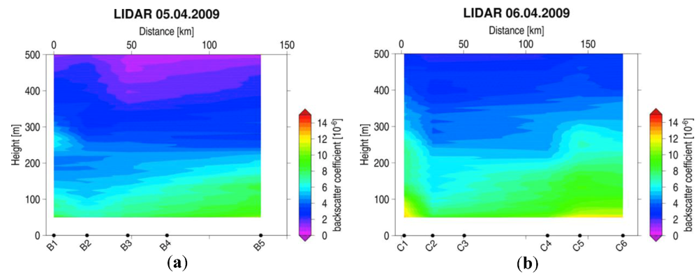
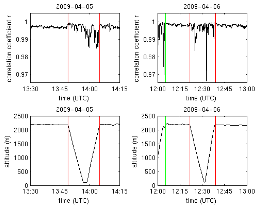
4.2. CASE B: The AABL above Sea Ice with a Relatively High Fraction of Open/Refrozen Leads

The measurements of case B took place close to Fram Strait under other ice conditions than cases C and D. In case B, we describe the sondes that are dropped over sea ice (B1–B6) with refrozen and partially open leads. Figure 4b shows a high resolution MODIS image with the flight track and the locations of dropsonde launches superimposed. While weather conditions were similar to those during the observations of case C (clear sky, winds from north-east, high solar radiation around noon, similar surface skin temperature above thick ice), the main difference was that the sea ice was more broken up with a higher number of larger refrozen leads, which influenced the lower atmosphere. Pictures of the surface below the aircraft taken during the measurements of dropsonde B3 (Figure 3a) and B5 (Figure 3b) reveal the existence of open/refrozen leads in the ice.

The near-surface temperature recorded by dropsonde measurements (Figure 5b) generally increased along the flight track towards the southeast. The northernmost profiles, near 81°N, exhibited a near-surface temperature of −30 °C. The near-surface temperature was about −26 °C at latitude 80°N. The temperature recorded on board of the POLAR-5 at 100 m altitude had a minimum around dropsonde B3 (Figure 10a). This corresponds to the locations where no areas of thin ice cover were recorded (Figure 10a). The surface skin temperature was about 7 K lower than the 100 m air temperature for areas above thick ice (e.g., between the location of dropsondes B3 and B4, Figure 10a), and the surface skin temperature was about 10 K higher than the 100 m air temperature above a broad region of refrozen leads (e.g., at a distance of 140 km in Figure 10a).

Figure 10. Data obtained during low-level flight segments of POLAR-5 on 5 (a), and 6 (b) April 2009. The x-axes indicate the distance from the first measurement and are oriented in north-south direction. The different panels indicate time series of the altitude (GPS signal), ice thickness, skin temperature, air temperature and relative humidity. The numbers in the uppermost panels indicate the location of the dropsondes launched on the outbound leg at higher altitudes. Wind data are not available. Panel (c) and (d) show aircraft data of altitude (GPS signal), Condensation Nucleus (CN) concentration, air temperature and relative humidity obtained on two flight legs on 10 April 2009, the flight to the NP-36 (c) at 2,000 m altitude (free atmosphere) and the flight to Alert in the boundary layer (d).

The depth of the AABL also varied significantly and systematically on April 5 while approaching the ice edge (Figure 4b and Figure 6b). The AABL was capped by a strong temperature inversion up to an altitude of 1,400 m (not shown). However, in the lowest 150–200 m, the profiles were modified. The near-surface temperature was higher than in case D (Figure 5d), and the surface temperature inversion was much less pronounced as above open water or absent (case A). The spatial variability of the near-neutral/weakly stable stratification in the lowest 150 m to 400 m can be seen in Figure 6b. Especially dropsondes B4 and B5, which were dropped in a region of larger leads, (Figure 10a) show higher altitudes of the strongest vertical gradient of potential temperature (red dots). It indicates vertical mixing and upward transport of sensible heat from the surface with partly open/refrozen leads. However, the 100 m air temperature shows a less clear signal (no significantly enhanced temperature directly above the large open leads). This could be attributed to the time and location shift compared to the dropsonde observations.

The ice thickness distribution measured with the EM Bird indicates a high frequency of 0.4 to 0.5 m thick new ice on refrozen leads (Figure 11, red line). The time series of ice thickness and skin temperature reveal lowest ice thickness and highest skin temperature simultaneously (Figure 10a). Both data sets indicate that the dimension of sections with open water (ice thickness 0 m, skin temperature −2 °C) was smaller than the footprint of the airborne sensors, i.e., <50 m for the ice-thickness sensor and <400 m for the skin temperature. However, the heat flux through the thin ice could act as the energy source for the mixing of the AABL above [44].

The time-height cross section of the water vapor mixing ratio exhibits an increase towards the south, where more open leads were present, and an increase above 300 m altitude, with lowest values around 0.25 g kg⁻¹ (Figure 7b). The wind direction for dropsondes B1–B3 was variable with altitude, between north and northeast (Figure 8b). A marked change in the wind direction occurred at 300 m. The wind speed increased towards the south (Figure 9b), with low and fluctuating values of 1–4 m s⁻¹ for dropsondes B1–B2. For dropsondes B1–B3, the wind speed increased from the surface to 200 m, then decreased up to about 300 m. The wind speed of dropsonde B5–B6 was almost constant (7–10 m s⁻¹) up to 300 m altitude.

Figure 11. Ice thickness distributions obtained on 5 and 6 April during low-level flight segments only (time series are shown in Figure 10(a,b)). Modal thicknesses of new ice on refrozen leads and multi-year ice were 0.4 m and 2.3 m on 5 April, and 0.5 m and 2.4 m on 6 April 2009, respectively (bin width 0.1 m).

The lidar backscatter ratio showed background values of clean Arctic air (1.1–1.3, corresponding to a backscatter coefficient of around 2 × 10⁻⁶ m⁻¹ sr⁻¹) above 500 m (not shown). The backscatter ratio was slightly enhanced at altitudes below 500 m with values of 2–4 (corresponding to a backscatter coefficient of around 3–5 × 10⁻⁶ m⁻¹ sr⁻¹), and even higher values of 4–7 (4–10 × 10⁻⁶ m⁻¹ sr⁻¹) at altitudes below 300 m (Figure 12a). Distinct structures of aerosol layers were observed. For instance, at the beginning of the observation (B1), there was a pronounced layer with maximum backscatter ratio at around 300 m altitude (Figure 12a).

Figure 12. Lidar measurements of the backscatter coefficient on 5 (a) and 6 (b) April 2009.

4.3. CASE C: The AABL above Sea Ice with a Relatively Low Fraction of Open Refrozen Leads

The lidar and dropsonde measurements of case C took place on a flight segment flown over closed sea ice with few open/refrozen leads near the ice edge on 6 April 2009 (Figure 4c, C1–C7). Figure 4c shows a high resolution MODIS image with the flight track and the locations of dropsonde launches superimposed. Figure 5c shows time-height cross-sections of the dropsonde temperature data. The near-surface temperature was −31 °C at latitude 82.5°N and increased to about −27 °C near 81°N.

The surface skin temperature was slightly (about 3 K) colder than the 100 m air temperature for areas above thick ice (e.g., at a distance of 140 km, Figure 10b) indicating the existence of a surface-based temperature inversion, but the surface skin temperature was about 7 K warmer than the 100 m air temperature above the small refrozen leads (e.g., above the refrozen lead between dropsondes C5 and C6) indicative of turbulent mixing near the surface.

In general, surface-based temperature inversions were observed. The inversion top was located at an altitude of about 800 m, topped by a layer having a nearly constant temperature up to 1,200 m (not shown). The potential temperature increased with altitude, showing a stably stratified air that inhibits vertical mixing (Figure 6c). The maximum vertical gradient of the potential temperature was at low altitudes (100–200 m for dropsondes C2–C6, red dots in Figure 6c). The water vapor mixing ratio derived from dropsonde observations (Figure 7c) was low at the lowest boundary and increased with height above the surface. A sharp increase was observed around 200 m. Surface level mixing ratios also increased towards the ice edge. The wind direction with easterly winds was almost constant with altitude (Figure 8c). The wind speed increased from low values near the surface (4 m s⁻¹) to around 8 m s⁻¹ at an altitude of 200 m (Figure 9c). The lidar profiles showed a high backscatter coefficient in the lowermost 200 m, and a smaller backscatter coefficient above (Figure 12b).

4.4. CASE D: The AABL above Closed Sea Ice with a Front Passing along the Flight Track

On 10 April 2009, the depth of the AABL varied along the flight track due to a frontal system. No areas of thin ice were recorded with the ice-thickness sensor (not shown). The top of the stable layer was located at about 200 m altitude north of 84.5° (location corresponding to dropsonde D3, Figure 4d and Figure 6d). The temperature data showed a strong surface-based temperature inversion (>10 K, Figure 5d). The dropsonde data evidenced the modulation of the AABL by synoptic forcing. The frontal location was calculated with a simple approach using the largest horizontal temperature gradient at each height interval (Figure 5d, black line with red dots). The air mass border (synoptic front, red line in Figure 5d, Figure 6d, Figure 7d, Figure 8d, Figure 9d) is obvious in the all data around 84.5°N (dropsonde D3, Figure 5d, Figure 6d, Figure 7d, Figure 8d, Figure 9d). The frontal surface can be seen to slope northward with height with warmer air to its south, and depth of the AABL and strength of the capping inversion change at this location. The transect of profiles from the dropsondes reveal the spatial variations across the front located at 84.5°N: The surface-based temperature inversion in the lowest 500 m is more pronounced before and after the front passage (Figure 5d, D1–D2, and D5–D16). A weakening of the surface based inversion due to mixing in the vicinity of the front is observed (Figure 5d, D3–D4). A change in wind direction from westerly to its south to easterly to its north (Figure 8d) is observed as well. The wind speed was lowest around the front and increased towards the north and south (Figure 9d). The altitude where the moisture increases (Figure 7d) was closely linked to the temperature inversion with higher moisture above the temperature inversion. The synoptic pattern underlying this transition is shown in Figure 2e, with a high-pressure system at the northern part of the flight leg and a low-pressure system at the southern part of the flight leg.

There are differences in the CN concentrations between boundary layer air and the free atmosphere in the region where the front has already passed (south of 84.5°N) and farther north, where the front has not yet passed: Figure 10c and d show the flight data, including the CN concentration on the way to NP-36 (Figure 10c) and on the way back to Alert (Figure 10d). On the way to NP-36, the data were obtained in the altitude range from 1,900–2,200 m in the free troposphere (Figure 10c). On the way back to Alert data were obtained in the altitude range from 50 to 200 m, i.e., within the AABL (Figure 10d). In the northern parts of the flights (north of 84.5°N, corresponding to locations left of D3 in Figure 10c), before the passage of the front, the CN concentration in the free troposphere was higher (>200 cm⁻³) than the concentration in the AABL (<200 cm⁻³). In the southern parts of the flights (south of 84.5°N, corresponding to locations right of D3 in Figure 10c), the CN concentration was higher in the AABL than in the free troposphere.

5. Discussion

5.1. Meteorology

Generally, the spatial variability of meteorological parameters like AABL height was high, and profiles changed significantly over a horizontal distance of about 250 km in all four cases (see Figure 5, Figure 6, Figure 7, Figure 8, Figure 9). The dropsonde temperature profiles can be divided into four cases as presented in Section 4, namely those observed above (I) open water, (II) a closed ice surface and (III) an ice cover with significant fraction of open and/or refrozen leads and (IV) an ice cover with only few open/refrozen leads. Warm near-surface temperatures and the lack of a temperature inversion corresponded to the atmosphere above open water (case A). A stable stratified atmosphere was observed above closed pack ice, with a temperature difference across the inversion layer of about 10 to 12 K in the central Arctic (case D, Figure 5d). The inversion during this case study was stronger than those reported in the climatology of dropsonde and radio sonde profiles from North Pole Drifting Stations from 1950 to 1990 [45]. The studies revealed mean temperature differences across the inversion layer of 6 K in April and 10 K in March. Similar temperature differences across surface inversions were recorded during winter in the Beaufort Sea region [46] as observed during PAMARCMiP. Our measurements contribute a new data set to the sparse observations in the central Arctic. The small-scale variations underline the importance of airborne observations covering large areas in the central Arctic.

In the presented observations, the characteristics of the AABL were strongly coupled to synoptic events and surface properties, namely sea ice with variable fraction and thickness of leads. Figure 11 shows ice thickness distributions obtained for case B (5 April, red line) and case C (6 April, blue line) on the outbound leg in the region where also the dropsondes were launched. Both distributions are bimodal, representing the occurrence of predominantly multi-year ice 2.3 to 2.4 m thick, as well as the presence of 0.4 to 0.5 m thick new ice on refrozen leads. Note that the fraction of refrozen leads was 7.4% for case B, much higher than the 2.1% for case C, while the older ice showed comparable thickness values at both locations.

We hypothesize that the observed differences in AABL depth of cases B and C are caused both by large-scale synoptic forcing and by different surface conditions, i.e., the lead fraction contained in the sea ice. The EM bird ice thickness data and skin temperature data show that both case B and case C had several regions of thinner ice (Figure 10(a,b)). The main difference between the two cases was that the track of case B went over some wide regions of thin ice (~3–9 km wide), especially towards the SE end of the track (sondes B4, B5) while the track of case C had smaller thin-ice areas (~50–200 m wide) throughout its entirety, which were not well resolved by the skin temperature measurements due to the large footprint. There was a wider thin-ice region of 4–6 km width between dropsondes C6 and C7. As some studies have shown [47], the width of the open leads (or in this case the thin-ice lead with warmer skin temperature and greater heat flux) plays an important role for the amount of heat that actually gets into the atmosphere. Hence, the multi-km wide thin ice of case B will likely produce larger impacts than will the more numerous smaller leads of case C. Above regions of thin ice cover (e.g., dropsondes B3 and B4), the AABL height was enhanced compared to sondes above thick ice (B1 and B2)

However, no clear correlation between surface skin temperature and the temperature recorded onboard the POLAR-5 at 100 m altitude was observed (Figure 10(a,b)). The penetration of convective plumes could be limited to altitudes barely reaching 100 m, which is in agreement with other observations and modeling results of similarly wide leads [44,48]. The time and location shift between dropsonde and airborne meteorological observations could be responsible for the different temperature effects observed by the two systems, with enhanced temperature only up to 100 m (airborne measurements) and visible up to several 100 m (dropsondes). The different AABL height observed for case B and C may be caused by synoptic differences. The low pressure system near Svalbard was more pronounced for case C (6 April) than for case B (5 April, (see Figure 2(a,b)). The stronger warm air advection above 500 m for case C (6 April), with a temperature increase above 500 m by 5 K (not shown), could induce large-scale subsidence, reducing the AABL height. Further, the different launch times of the dropsondes (case B: early afternoon, case C: around noon) could be a factor influencing the AABL height, as the mixing height should grow with solar radiation and a maximum can be expected directly after noon (case B).

Figure 13. Correlation coefficient r between F_sc and C (upper panels) and flight altitude (lower panels) on 5 (left) and 6 (right) April 2009. The red vertical lines mark the beginning of a descent and the end of a subsequent ascent during the time periods investigated. Similarly, the green vertical line marks the end of an ascent. For the horizontal flight legs, the very high correlation coefficient r with values always larger than 0.995 indicates the absence of clouds.

To exclude the presence of clouds above the aircraft, we analyzed measurements of broadband solar downwelling hemispheric radiation flux densities for the time period 13:30 UTC to 14:15 UTC on 5 April 2009 (case B) and for the period 12:00 UTC to 13:00 UTC on 6 April 2009 (case C). Under homogeneous conditions and the absence of clouds, the sensor signals of the upper pyranometer depend significantly on the aircraft’s roll and pitch angles. The global radiation F_swdown can be decomposed into an isotropic diffuse part F_diff and a direct solar part F_dir (F_swdown = F_diff + F_dir, [39]). These parts are obtained as regression parameters of the linear equation F_sc = F_diff + F_dir (cos β/cos θ), where F_sc are the corrected flux densities after calibration and correction for the instrumental lag, β is the angle between the pyranometer zenith and the sun [49], and θ is the solar zenith angle. Under homogeneous conditions and the absence of clouds, there is a linear dependence of F_sc on the parameter C = cos β/cos θ. For horizontal flight attitude (C = 1), the measurements provide the global radiation. For C ≠ 1, the measurements have to be corrected for the roll and pitch angles. For the two time periods selected for case B and C, we calculated every 50 ms (measurement frequency) the correlation coefficient r between the values of F_sc and of C obtained in time intervals of 60 s. Figure 13 shows the results for case B (left panels) and case C (right panels). The correlation coefficient r never drops below 0.995 for the horizontal flight legs on both days. Such a high correlation coefficient r between F_sc and C indicates that clouds, which cause inhomogeneities in the radiation field, were completely absent. In the presence of clouds, the correlation coefficient usually drops down to values (considerably) lower than 0.9, depending on cloud type [50]. Clouds below the flight altitude can be excluded by the nadir lidar observations, which are very sensitive in detecting even thin layers of subvisible clouds [51].

The difference between surface skin temperature and 100 m air temperature was similar for both cases above refrozen leads (surface about 7 K warmer). Above thick ice, the difference between the colder skin temperature and the 100 m air temperature was more pronounced for case B (about 7 K) than for case C (2–3 K). Considering only the temperature gradient above ice, the AABL should be more stable for case B with the more pronounced temperature inversion. For case B, the thermal profiles with a well-mixed structure near the surface over sea ice could be caused by heat flux through the thin ice on refrozen leads. A sensitivity study determining the influence of sea ice thickness on thermodynamics showed that the sensible heat flux over ice thinner than 0.8 m was still directed towards the atmosphere, as the skin temperature was warmer than the air temperature [52]. For ice thickness between 0.2–0.4 m, the sensible heat flux may be as large as 100 W m⁻². This was also confirmed by satellite-derived data for ice thickness and sensible heat flux for Arctic polynyas [53]. Impacts of refreezing leads in terms of enhanced sensible and latent heat fluxes and a decrease in atmospheric stability were reported downwind of the lead up to 60 m altitude [48]. The (upward) heat fluxes above areas of thin ice compensate the downward heat fluxes above thick ice in a way that the sensible heat flux is around zero on a regional scale in winter [13]. Large heat fluxes for individual leads were observed in the lowest 30 m [54]. The vertical extent of plumes above leads depends on the thermal structure of the atmosphere, with stable stratifications prohibiting the development of large plumes above leads, and neutral stratification, e.g., after a front, allowing deeper plume penetration [22,47].

A mixed layer can also occur over snow-covered ice with sufficient solar radiation (or another heat source) warming the surface [11]. We can exclude that the surface-based mixed layer occurred due to positive net IR radiation resulting from clouds (see above) and conductive heat flux through the thick ice. Photographic pictures taken during the dropsonde launches provide evidence of open and refrozen leads along the flight path (Figure 3). Also the analysis of the ice thickness shows the presence of refrozen leads (Figure 11).

A turbulent boundary layer in the vicinity of leads is often capped by a stable layer having a strong inversion [48]. A change of the wind direction, wind speed and water vapor mixing ratio is commonly observed above such a stable layer [10]. In case B, the boundary layer extended up to 300 m altitude, while in case C, the boundary layer extended up to only 200 m (Figure 6(b,c)). As the surface skin temperature above thick ice was similar for both cases, we attribute the differences to the fact that the ice surface was more coherent in case C.

A stably stratified AABL, characterized by an increasing potential temperature with altitude, is usually observed above solid pack ice (case D). The top of the AABL of our observations, marked by a prominent change in wind speed, wind direction, and relative humidity, is comparable to the boundary-layer height above sea ice reported by other groups: Near-neutral and weakly stable stratification was observed directly from the surface up to 250 m with a strong temperature inversion above during helicopter-based turbulence measurements made above the solid pack ice in the Kara Sea and East Siberian Sea during July/August 1996 [55]. A boundary layer vertical extent of 100–300 m above sea ice was reported during March (late winter) with similar values of near-surface temperature and specific humidity as reported here, as well as increasing moisture with altitude [9]. Increasing specific humidity above the boundary layer was also a common observation during the Arctic Ocean Experiment in July/August 2001 [56]. Our observations of a relatively dry boundary layer over closed sea ice are in agreement with some dropsonde measurements [57]; however, they are in contrast to the airborne in situ and dropsonde measurements obtained in the Davis Strait in April 1997, where enhanced specific humidity in the stably stratified boundary layer close to the sea ice edge was reported [58].

For case B, we observed vertical variations in wind speed (Figure 9b) and direction (Figure 8b), which seem to have a vertical wavelength of 200 m for the dropsondes B1–B3. These structures can also be seen in the lidar backscatter profiles (Figure 12a). Such wave-like features have been observed by other airborne measurements in the stably stratified Arctic boundary layer over ice with open leads [43]. These are thought to be induced by gravity waves and small-scale horizontal roll vortices generated by convection over the leads [43]. Although no areas of thin ice were recorded around dropsondes B1–B3 (Figure 10a), nearby leads may be present which could be responsible for this effect.

5.2. Aerosol Load in the Central Arctic

The columnar aerosol burden observed during PAMARCMiP was overall higher in comparison with previous years [59,60]. Values of AOD at 500 nm during the campaign, derived from Sun photometer data, varied from about 0.12 to >0.35 [25]. Air in the vicinity of Svalbard in early April was significantly less turbid than air over the Beaufort Sea region during the third week of the field campaign in April 2009. Despite relatively high values of total light extinction, black carbon concentrations were moderately low during the flights (Figure 7(c,f) in [25]) compared with historical observations [61]. Similar measurements of BC were obtained from a series of flights during the Arctic Gas and Aerosol Sampling Program (AGASP) in 1983 and 1986 [62].

The source of aerosols, which were mainly confined to low levels, was from Eurasia through most of April, with an Asian component towards the end of the campaign. Some enhancement from normal background conditions in the upper troposphere was also observed, attributed to a combination of volcanic aerosol from eruptions of Redoubt in Alaska and emissions from industrial regions at mid latitudes. We analyzed mean back-trajectories calculated from an ensemble of 1,000 trajectories with the Pole-Equator-Pole (PEP) tracer model, which employs a uniform computation scheme all around the globe, avoiding special treatment of high latitudes [63]. While the source of haze was in general from Eurasia during April 2009 [25], the trajectories of case B and C for the aircraft locations investigated here (Figure 14(a,b)) indicate that the flow was mainly from the North American sector and over the North Pole during these two days, where it likely mixed with pollutants accumulated within the high Arctic.

For case D, CN measurements were obtained at two different altitudes, once in the free troposphere at altitudes between 1,900 and 2,200 m (Figure 10c) and once within the AABL (Figure 10d) at altitudes between 50 and 200 m. In the southern parts of the flight legs (south of 84.5°N, corresponding to dropsonde D3), the CN concentration in the free troposphere was clearly lower than the CN concentration in the AABL. This is the area where the front system has already passed. The front is associated with vertical mixing, leading to downward transport of long-range aerosol into the AABL. In the northern parts of the flight legs (north of 84.5°N), the CN concentration in the free troposphere was higher than in the AABL. Due to large-scale advection, the free troposphere in the high-pressure region north of 84.5°N revealed a higher CN concentration than the low pressure region south of the synoptic front (Figure 10c). Along the front, cold air with high CN concentration slides down, while clean boundary layer air is lifted upwards. Thus on the flight back, higher CN concentrations are found in the boundary layer south of the synoptic front, where vertical mixing due to the cyclonic activity has already occurred (Figure 10d). Relatively high AOD aloft near NP-36 was also observed (Figure 7 in [24]), which corroborates the enhanced free-troposphere aerosol burden at this high latitude. Because there are no local sources of aerosol in the region, aged aerosol trapped or transported into the region probably underlies the observed enhancement. These haze particles do not function effectively as ice nuclei (IN). Even at temperatures as low as −25 °C, pollutants tend to have very low IN/CN ratios and slow nucleation rates [64]. The characteristics of Arctic haze tend to suppress wet deposition, which enables haze to survive long‐range transport and accumulate within the Arctic atmosphere. It follows that ineffectual nucleation may suppress the deposition of soot onto the ice/snow surface. Moreover, the Arctic atmosphere is highly stratified, reducing vertical mixing and re-distribution of the aerosol to the surface.

Figure 14. Correlation PEP mean backward trajectories calculated from ensemble trajectories along the flight track on 5 April 2009 at 13:38 (a), on 6 April 2009 at 12:43 (b), and on 10 April 2009 at 14:02 (c) and 16:02 UTC (d). The ensembles consist of a set of trajectories with starting positions distributed around the point of interest (here the aircraft location at a given time) in uniform density. The colors represent the pressure levels, 950 hPa (blue), 850 hPa (green), 700 hPa (red) and 500 hPa (orange). Stars are set for every day. On 5 and 6 April, backward trajectories are calculated for six days. On 10 April, trajectories are calculated for 12 days. Stars are set for every two days.

We analyzed the origin of the air masses for two different locations along the flight path with mean backward trajectories from ensembles computed with PEP-Tracer. South of 84.5°N, where the front has already passed and vertical mixing has taken place (Figure 14c), the backward trajectories indicate a similar path for all altitudes. North of 84.5°N, the trajectories in the free atmosphere (700 hPa) show long-range transport from Eurasia, while the trajectories in the AABL (950 hPa) are confined to the high Arctic. This may explain the higher CN values in the free troposphere at latitudes north of 84.5°N. The analyses of mean trajectories support the hypothesis that the origin of the air masses at different altitudes change when the front passed. This implies distinct properties of the analyzed air masses and especially the aerosol load at different altitudes, which was observed by dropsonde and particle concentration.

6. Conclusions

Measurements of the AABL in the central Arctic were obtained within a few days above different surface conditions (open water, closed sea ice and sea ice containing different fractions of open/refrozen leads) by simultaneous backscatter lidar and dropsonde profiles. Additionally, airborne in situ meteorological and aerosol concentration measurements as well as ice thickness observations were analyzed. We found a large spatial variability of atmospheric parameters like the AABL depth on a scale of a few 100 km, which was attributed to synoptic influences (the flight track passing through a front) and differences in surface ice conditions. Based on our observations, we came to the following conclusions:

Closed sea ice supports the development of a very stable and shallow AABL, while open water in average is more related to a neutral stratification. However, AABL altitude and structure depend on many other factors, such as synoptic fronts. For our observations, we considered only cloud-free conditions.

The aerosol load is not a good tracer for the AABL height, as the backscatter coefficient almost always shows a smooth increase towards the ground and moreover sporadically elevated layers. Hence one cannot simply take the largest gradient in lidar signal for AABL height determination in the Arctic.

Similarly, the largest vertical gradient in relative humidity is not a good tracer for the AABL height, as the relative humidity is too variable. Open leads affect the relative humidity only up to several 10 m, while the air temperature may be influenced simultaneously up to more than 100 m altitude.

Aerosol properties are directly related to the thermodynamic state of the atmosphere. The CN in situ concentration in the AABL and the free troposphere are reversed by the vertical mixing processes associated with a passing front.

For future advances in understanding atmospheric processes in the central Arctic, similar comprehensive data sets covering larger areas are essential to quantify the influences of different factors controlling the AABL characteristics.

Acknowledgments

The authors would like to thank the flight crew of the POLAR-5, namely Captain Brian Burchartz, co-pilot Andrew Jenkins and mechanic Timothy Anderson, and all from the POLAR-5 operator Enterprise Airline Inc. Oshawa. We would like to thank Holger Deckelmann for help with the MODIS images, contour plots and aircraft data. We acknowledge the use of NASA/GSFC MODIS Rapid Response data. Further, we thank two reviewers for their valuable comments.

References

Allison, I.; Beland, M.; Alverson, K.; Bell, R.; Carlson, D.; Danell, K.; Ellis-Evans, C.; Fahrbach, E.; Fanta, E.; Fujii, Y.; Glaser, G.; Goldfarb, L.; Hovelsrud, G.; Huber, J.; Kotlyakov, V.; Krupnik, I.; Lopez-Martinez, J.; Mohr, T.; Qin, D.; Rachold, V.; Rapley, C.; Rogne, O.; Sarukhabian, E.; Summerhayes, C.; Xiao, C. The Scope of Science for the International Polar Year 2007/2008; WMO/TD-No. 1364. World Meteorological Organization: Geneva, Switzerland, 2007; p. 79. [Google Scholar]
Vance, A.K.; Taylor, J.P.; Hewison, T.J.; Elms, J. Comparison of in situ humidity data from aircraft, dropsonde, and radiosonde. J. Atmos. Ocean. Technol. 2004, 21, 921–932. [Google Scholar] [CrossRef]
Shupe, M.D.; Uttal, T.; Matrosov, S.Y. Arctic cloud microphysics retrievals from surface-based remote sensors at SHEBA. J. Appl. Meteorol. 2005, 44, 1544–1562. [Google Scholar] [CrossRef]
Kahl, J.D.W.; Zaitseva, N.A.; Khattatov, V.; Schnell, R.C.; Bacon, D.M.; Bacon, J.; Radionov, V.; Serreze, M.C. Radiosonde observations from the former Soviet “north pole” series of drifting ice stations, 1954–1990. Bull. Am. Meteorolog. Soc. 1999, 80, 2019–2026. [Google Scholar] [CrossRef]
Beesley, J.A.; Bretherton, C.S.; Jakob, C.; Andreas, E.L.; Intrieri, J.M.; Uttal, T.A. A comparison of cloud and boundary layer variables in the ECMWF forecast model with observations at Surface Heat Budget of the Arctic Ocean (SHEBA) ice camp. J. Geophys. Res. 2000, 105, 12337–12349. [Google Scholar]
Dethloff, K.; Abegg, C.; Rinke, A.; Hebestadt, I.; Romanov, V.F. Sensitivity of Arctic climate simulations to different boundary-layer parameterizations in a regional climate model. Tellus 2001, 53A, 1–26. [Google Scholar]
Tjernström, M.; Zagar, M.; Svensson, G.; Cassano, J.J.; Pfeifer, S.; Rinke, A.; Wyser, K.; Dethloff, K.; Jones, C.; Semmler, T.; Shaw, M. Modelling the Arctic boundary layer: An evaluation of six ARCMIP regional-scale models using data from the SHEBA project. Bound. Lay. Meteorol. 2005, 117, 337–381. [Google Scholar] [CrossRef]
Dorn, W.; Dethloff, K.; Rinke, A. Limitations of a coupled regional climate model in the reproduction of the observed Arctic sea-ice retreat. Cryosphere Discuss. 2012, 6, 1269–1306. [Google Scholar] [CrossRef]
Curry, J.A.; Ebert, E.E.; Herman, G.F. Mean and turbulence structure of the summertime Arctic cloudy boundary layer. Q.J.R. Meteorol. Soc. 1988, 114, 715–746. [Google Scholar] [CrossRef]
Brümmer, B. Boundary-layer modification in wintertime cold-air outbreaks from the Arctic sea ice. Bound. Lay. Meteorol. 1996, 80, 109–125. [Google Scholar] [CrossRef]
Persson, P.O.G.; Fairall, C.W.; Andreas, E.L.; Guest, P.S.; Perovich, D.K. Measurements near the atmospheric surface flux group tower at SHEBA: Near-surface conditions and surface energy budget. J. Geophys. Res. 2002, 107. [Google Scholar] [CrossRef]
Duynkerke, P.G.; De Roode, S.R. Surface energy balance and turbulence characteristics observed at the SHEBA ice camp during FIRE III. J. Geophys. Res. 2001, 106, 15313–15322. [Google Scholar] [CrossRef]
Overland, J.E.; McNutt, S.L.; Groves, J.; Salo, S.; Andreas, E.L.; Persson, P.O.G. Regional sensible and radiative heat flux estimates for the winter Arctic during the Surface Heat Budget of the Arctic Ocean (SHEBA) experiment. J. Geophys. Res. 2000, 105, 14093–14102. [Google Scholar] [CrossRef]
Brümmer, B.; Busack, B.; Hoeber, H.; Kruspe, G. Boundary-layer observations over water and Arctic sea-ice during on-ice air flow. Bound. Lay. Meteorol. 1994, 68, 75–108. [Google Scholar] [CrossRef]
Curry, J.A.; Hobbs, P.V.; King, M.D.; Randall, D.A.; Minnis, P.; Isaac, G.A.; Pinto, J.O.; Uttal, T.; Bucholtz, A.; Cripe, D.G.; Gerber, H.; Fairall, C.W.; Garrett, T.J.; Hudson, J.; Intrieri, J.M.; Jakob, C.; Jensen, T.; Lawson, P.; Marcotte, D.; Nguyen, L.; Pilewskie, P.; Rangno, A.; Rogers, D.C.; Strawbridge, K.B.; Valero, F.P.J.; Williams, A.G.; Wylie, D. Fire Arctic clouds experiment. Bull. Am. Meteorol. Soc. 2000, 81, 5–29. [Google Scholar]
Vihma, T.; Hartmann, J.; Lüpkes, C. A case study of an on-ice air flow over the Arctic marginal sea-ice zone. Bound. Lay. Meteorol. 2003, 107, 189–217. [Google Scholar] [CrossRef]
Zuidema, P.; Baker, B.; Han, Y.; Intrieri, J.; Key, J.; Lawson, P.; Matrosov, S.; Shupe, M.; Stone, R.; Uttal, T. An Arctic springtime mixed-phase cloudy boundary layer observed during SHEBA. J. Atmos. Sci. 2005, 62, 160–176. [Google Scholar] [CrossRef]
Lüpkes, C.; Schlünzen, K.H. Modelling the Arctic convective boundary-layer with different turbulence parameterizations. Bound. Lay. Meteorol. 1996, 79, 107–130. [Google Scholar] [CrossRef]
Serreze, M.C.; Maslanik, J.A.; Rheder, M.C.; Schnell, R.C.; Kahl, J.D.; Andreas, E.L. Theoretical heights of buoyant convection above open leads in the winter Arctic pack ice cover. J. Geophys. Res. 1992, 97, 9411–9422. [Google Scholar] [CrossRef]
Dare, R.A.; Atkinson, B.W. Atmospheric response to spatial variations in concentration and size of polynyas in the Southern ocean sea-ice zone. Bound. Lay. Meteorol. 2000, 94, 65–88. [Google Scholar] [CrossRef]
Guest, P.S. Measuring turbulent heat fluxes over leads using kites. J. Geophys. Res. 2007, 112. [Google Scholar] [CrossRef]
Schnell, R.C.; Barry, R.G.; Miles, M.W.; Andreas, E.L.; Radke, L.F.; Brock, C.A.; McCormick, M.C.; Moore, J.L. Lidar detection of leads in Arctic sea ice. Lett. Nat. 1989, 339, 530–532. [Google Scholar] [CrossRef]
Andreas, E.L.; Cash, B.A. Convective heat transfer over wintertime leads and polynyas. J. Geophys. Res. 1999, 104, 25721–25734. [Google Scholar] [CrossRef]
Lüpkes, C.; Vihma, T.; Birnbaum, G.; Wacker, U. Influence of leads in sea ice on the temperature of the atmospheric boundary layer during polar night. Geophys. Res. Lett. 2008, 35. [Google Scholar] [CrossRef] [Green Version]
Stone, R.; Herber, A.; Vitale, V.; Mazzola, M.; Lupi, A.; Schnell, R.; Dutton, E.; Liu, P.; Li, S.-M.; Dethloff, K.; Lampert, A.; Ritter, C.; Stock, M.; Neuber, R.; Maturilli, M. A three-dimensional characterization of Arctic aerosols from airborne sun photometer observations: PAM-ARCMIP—April 2009. J. Geophys. Res. 2010, 115. [Google Scholar] [CrossRef]
Shaw, G.E. Evidence for a central eurasian source area of Arctic haze in Alaska. Nature 1982, 299, 815–818. [Google Scholar] [CrossRef]
Warneke, C.; Bahreini, R.; Brioude, J.; Brock, C.A.; de Gouw, J.A.; Fahey, D.W.; Froyd, K.D.; Holloway, J.S.; Midlebrook, A.; Miller, L.; Montzka, S.; Murphy, D.M.; Peischl, J.; Ryerson, T.B.; Schwarz, J.P.; Spackman, J.R.; Veres, P. Biomass burning in Siberia and Kazakhstan as an important source for haze over the Alaskan Arctic in April 2008. Geophys. Res. Lett. 2009, 36. [Google Scholar] [CrossRef]
Devasthale, A.; Tjernström, M.; Omar, A.H. The vertical distribution of thin features over the Arctic analysed from CALIPSO observations, Part II: Aerosols. Tellus 2011, 63B, 86–95. [Google Scholar]
Spackman, J.R.; Gao, R.S.; Neff, W.D.; Schwarz, J.P.; Watts, L.A.; Fahey, D.W.; Holloway, J.S.; Ryerson, T.B.; Peischl, J.; Brock, C.A. Aircraft observations of enhancement and depletion of black carbon mass in the springtime Arctic. Atmos. Chem. Phys. 2010, 10, 9667–9680. [Google Scholar] [CrossRef]
McFarquhar, G.; Ghan, S.; Verlinde, J.; Korolev, A.; Strapp, J.W.; Schmid, B.; Tomlinson, J.M.; Wolde, M.; Brooks, S.D.; Cziczo, D.; Dubey, M.K.; Fan, J.; Flynn, C.; Gultepe, I.; Hubbe, J.; Gilles, M.K.; Laskin, A.; Lawson, P.; Leaitch, W.R.; Liu, P.; Liu, X.; Lubin, D.; Mazzoleni, C.; Macdonald, A.-M.; Moffet, R.C.; Morrison, H.; Ovchinnikov, M.; Shupe, M.D.; Turner, D.D.; Xie, S.; Zelenyuk, A.; Bae, K.; Freer, M.; Glen, A. Indirect and semi-direct aerosol campaign (ISDAC): The impact of Arctic aerosols on clouds. Bull. Amer. Meteorol. Soc. 2011, 92, 183–201. [Google Scholar]
Jacob, D.J.; Crawford, J.H.; Maring, H.; Clarke, A.D.; Dibb, J.E.; Emmons, L.K.; Ferrare, R.A.; Hostetler, C.A.; Russell, P.B.; Singh, H.B.; Thompson, A.M.; Shaw, G.E.; McCauley, E.; Pederson, J.R.; Fisher, J.A. The Arctic research of the composition of the troposphere from aircraft and satellites (ARCTAS) mission: Design, execution, and first results. Atmos. Chem. Phys. 2010, 10, 5191–5212. [Google Scholar]
Paatero, J.; Vaattovaara, P.; Vestenius, M.; Meinande, O.; Makkonen, U.; Kivi, R.; Hyvärinen, A.; Asmi, E.; Tjernström, M.; Leck, C. Finnish contribution to the Arctic summer cloud ocean study (ASCOS) expedition, Arctic ocean 2008. Geophysica 2009, 45, 119–146. [Google Scholar]
Sedlar, J.; Tjernström, M.; Mauritsen, T.; Shupe, M.D.; Brooks, I.M.; Persson, P.O.G.; Birch, C.E.; Leck, C.; Sirevaag, A.; Nicolaus, M. A transitioning Arctic surface energy budget: The impacts of solar zenith angle, surface albedo and cloud radiative forcing. Clim. Dyn. 2011, 37, 1643–1660. [Google Scholar] [CrossRef] [Green Version]
Persson, P.O.G. Summary of Meteorological Conditions during the Arctic Mechanisms for the Interaction of the Surface and Atmosphere (AMISA) Intensive Observation Periods; NOAA: Silver Spring, MD, USA. Available online: http://www.lib.muohio.edu/multifacet/record/mu3ugb4202658 (accessed on 10 November 2011).
Stachlewska, I.; Neuber, R.; Lampert, A.; Ritter, C.; Wehrle, G. AMALi—The Airborne Mobile Aerosol Lidar for Arctic research. Atmos. Chem. Phys. 2010, 10, 2947–2963. [Google Scholar]
Stone, R.S. Monitoring Aerosol Optical Depth at Barrow, Alaska and South Pole: Historical Overview, Recent Results, and Future Goals. In Proceedings of the 9th Workshop Italian Research on Antarctic Atmosphere, Bologna, Italy, 22–24 October 2002; Colacino, M., Ed.; pp. 123–144.
Haas, C.; Hendricks, S.; Eicken, H.; Herber, A. Synoptic airborne thickness surveys reveal state of Arctic sea ice cover. Geophys. Res. Lett. 2010, 37. [Google Scholar] [CrossRef] [Green Version]
Haas, C.; Lobach, J.; Hendricks, S.; Rabenstein, L.; Pfaffling, A. Helicopter-borne measurements of sea ice thickness, using a small and lightweight, digital EM system. J. Appl. Geoph. 2009, 67, 234–241. [Google Scholar] [CrossRef] [Green Version]
Freese, D.; Kottmeier, C. Radiation exchange between stratus clouds and polar marine surfaces. Bound. Lay. Meteorol. 1998, 87, 331–356. [Google Scholar] [CrossRef]
Wang, K.; Wan, Z.; Wang, P.; Sparrow, M.; Liu, J.; Zhou, X.; Haginoya, S. Estimation of surface long wave radiation and broadband emissivity using moderate resolution imaging spectroradiometer (MODIS) land surface temperature/emissivity products. J. Geophys. Res. 2005. [Google Scholar] [CrossRef]
Guenther, B.; Xiong, X.; Salomonson, V.V.; Barnes, W.L.; Young, J. On-orbit performance of the earth observing system (EOS) moderate resolution imaging spectroradiometer (MODIS) and the Attendant Level 1-B Data Product. Remote Sens. Environ. 2002, 83, 16–30. [Google Scholar] [CrossRef]
The Generic Mapping Tools. Available online: http://gmt.soest.hawaii.edu/ (accessed 1 April 2012).
Paluch, I.R.; Lenschow, D.H.; Wang, Q. Arctic boundary layer in the fall season over open and frozen sea. J. Geophys. Res. 1997, 102, 25955–25971. [Google Scholar]
Ruffieux, D.; Persson, P.O.G.; Fairall, C.W.; Wolfe, D.E. Ice pack and lead surface energy budget during LEADEX 1992. J. Geophys. Res. 1995, 100, 4593–4612. [Google Scholar]
Kahl, J.D.W.; Martinez, D.A.; Zaitseva, N.A. Long-term variability in the low-level inversion layer over the Arctic ocean. Int. J. Climatol. 1996, 16, 1297–1313. [Google Scholar]
Overland, J.E. Meteorology of the Beaufort sea. J. Geophys. Res. 2009, 114. [Google Scholar] [CrossRef]
Burk, S.D.; Fett, R.W.; Englebretson, R.E. Numerical simulation of cloud plumes emanating from Arctic leads. J. Geophys. Res. 1997, 102, 16,529–16,544. [Google Scholar]
Lüpkes, C.; Vihma, T.; Birnbaum, G.; Dierer, S.; Garbrecht, T.; Gryanik, V.M.; Gryschka, M.; Hartmann, J.; Heinemann, G.; Kaleschke, L.; Raasch, S.; Savijärvi, H.; Schlünzen, K.H.; Wacker, U. Arctic Climate Change: The ACSYS Decade and Beyond; Springer Science and Business Media: New York, NY, USA, 2012; Volume Chapter 7, pp. 279–324. [Google Scholar]
Bannehr, L.; Schwiesow, R. A technique to account for the misalignment of pyranometers installed on aircraft. J. Atmos. Ocean. Tech. 1993, 10, 774–777. [Google Scholar] [CrossRef]
Freese, D. Solar and Terrestrial Radiation Interaction between Arctic Sea Ice and Clouds; Report on Polar Research No. 312; Alfred Wegener Institute: Bremerhaven, Germany, 1999. [Google Scholar]
Lampert, A.; Ehrlich, A.; Dörnbrack, A.; Jourdan, O.; Gayet, J.-F.; Mioche, G.; Shcherbakov, V.; Ritter, C.; Wendisch, M. Microphysical and radiative characterization of a subvisible midlevel arctic ice cloud by airborne observations—A case study. Atmos. Chem. Phys. 2009, 9, 2647–2661. [Google Scholar]
Schramm, J.L.; Holland, M.M.; Curry, J.A.; Ebert, E.E. Modeling the thermodynamics of a sea ice thickness distribution 1. Sensitivity to ice thickness resolution. J. Geophys. Res. 1997, 102, 23079–23091. [Google Scholar] [CrossRef]
Martin, S.; Drucker, R.; Kwok, R.; Holt, B. Estimation of the thin ice thickness and heat flux for the Chukchi Sea Alaskan coast polynya from special sensor microwave/imager data, 1990–2001. J. Geophys. Res. 2004, 109. [Google Scholar] [CrossRef]
Walter, B.A.; Overland, J.E.; Turet, P. A comparison of satellite-derived and aircraft-measured regional surface sensible heat fluxes over the Beaufort Sea. J. Geophys. Res. 1995, 100, 4585–4591. [Google Scholar] [CrossRef]
Van den Kroonenberg, A.; Bange, J. Turbulent flux calculation in the polar stable boundary layer: Multiresolution flux decomposition and wavelet analysis. J. Geophys. Res. 2007, 112. [Google Scholar] [CrossRef]
Tjernström, M.; Leck, C.; Persson, P.O.G.; Jensen, M.L.; Oncley, S.P.; Targino, A. The summertime Arctic atmosphere: Meteorological measurements during the Arctic Ocean Experiment 2001 (AOE-2001). Bull. Am. Meteorol. Soc. 2004, 85, 1305–1321. [Google Scholar] [CrossRef]
Pinto, J.O. Autumnal mixed-phase cloudy boundary layers in the Arctic. J. Atmos. Sci. 1998, 55, 2016–2038. [Google Scholar] [CrossRef]
Drüe, C.; Heinemann, G. Airborne investigation of Arctic boundary-layer fronts over the marginal ice zone of the Davis Strait. Bound. Lay. Meteorol. 2001, 101, 261–292. [Google Scholar] [CrossRef]
Hoffmann, A.; Ritter, C.; Stock, M.; Shiobara, M.; Lampert, A.; Maturilli, M.; Orgis, T.; Neuber, R.; Herber, A. Ground-based lidar measurements from Ny-Ålesund during ASTAR 2007. Atmos. Chem. Phys. 2009, 9, 9059–9081. [Google Scholar] [CrossRef]
Hoffmann, A.; Osterloh, L.; Stone, R.; Lampert, A.; Ritter, C.; Stock, M.; Tunved, P.; Hennig, T.; Böckmann, C.; Li, S.-M.; Eleftheriadis, K.; Maturilli, M.; Orgis, T.; Herber, A.; Neuber, R.; Dethloff, K. Remote sensing and in-situ measurements of tropospheric aerosol, a PAMARCMiP case study. Atmos. Environ. 2012, 52, 56–66. [Google Scholar] [CrossRef] [Green Version]
Dutton, E.G.; Deluisi, J.J.; Herbert, G. Shortwave aerosol optical depth of Arctic haze measured on board the NOAA WP-3D during AGASP-II, April 1986. J. Atmos. Chem. 1989, 9, 71–79. [Google Scholar] [CrossRef]
Hansen, A.D.A.; Novakov, T. Aerosol black carbon measurements in the Arctic haze during AGASP-II. J. Atmos. Chem. 1989, 9, 347–361. [Google Scholar] [CrossRef]
Orgis, T.; Brand, S.; Schwarz, U.; Handorf, D.; Dethloff, K.; Kurths, J. Influence of interactive stratospheric chemistry on large-scale air mass exchange in a global circulation model. Eur. Phys. J. 174, 257–269.
Borys, R.D. Studies of ice nucleation by Arctic aerosol on AGASP-II. J. Atmos. Chem. 1989, 9, 169–185. [Google Scholar] [CrossRef]

© 2012 by the authors; licensee MDPI, Basel, Switzerland. This article is an open-access article distributed under the terms and conditions of the Creative Commons Attribution license (http://creativecommons.org/licenses/by/3.0/).

Share and Cite

MDPI and ACS Style

Lampert, A.; Maturilli, M.; Ritter, C.; Hoffmann, A.; Stock, M.; Herber, A.; Birnbaum, G.; Neuber, R.; Dethloff, K.; Orgis, T.; et al. The Spring-Time Boundary Layer in the Central Arctic Observed during PAMARCMiP 2009. Atmosphere 2012, 3, 320-351. https://doi.org/10.3390/atmos3030320

AMA Style

Lampert A, Maturilli M, Ritter C, Hoffmann A, Stock M, Herber A, Birnbaum G, Neuber R, Dethloff K, Orgis T, et al. The Spring-Time Boundary Layer in the Central Arctic Observed during PAMARCMiP 2009. Atmosphere. 2012; 3(3):320-351. https://doi.org/10.3390/atmos3030320

Chicago/Turabian Style

Lampert, Astrid, Marion Maturilli, Christoph Ritter, Anne Hoffmann, Maria Stock, Andreas Herber, Gerit Birnbaum, Roland Neuber, Klaus Dethloff, Thomas Orgis, and et al. 2012. "The Spring-Time Boundary Layer in the Central Arctic Observed during PAMARCMiP 2009" Atmosphere 3, no. 3: 320-351. https://doi.org/10.3390/atmos3030320

Article Menu

The Spring-Time Boundary Layer in the Central Arctic Observed during PAMARCMiP 2009

Abstract

1. Introduction

2. Instrumentation

2.1. Dropsonde System

2.2. Lidar System

2.3. Aerosol Instrumentation

2.4. Ice-Thickness Sensor

2.5. Meteorological Instrumentation

3. Meteorological Situation

4. Airborne Observations

4.1. CASE A: The AABL above Open Water

4.2. CASE B: The AABL above Sea Ice with a Relatively High Fraction of Open/Refrozen Leads

4.3. CASE C: The AABL above Sea Ice with a Relatively Low Fraction of Open Refrozen Leads

4.4. CASE D: The AABL above Closed Sea Ice with a Front Passing along the Flight Track

5. Discussion

5.1. Meteorology

5.2. Aerosol Load in the Central Arctic

6. Conclusions

Acknowledgments

References

Share and Cite

Article Metrics

Article Access Statistics

Further Information

Guidelines

MDPI Initiatives

Follow MDPI