Emission Ratios for Ammonia and Formic Acid and Observations of Peroxy Acetyl Nitrate (PAN) and Ethylene in Biomass Burning Smoke as Seen by the Tropospheric Emission Spectrometer (TES)

Abstract
: We use the Tropospheric Emission Spectrometer (TES) aboard the NASA Aura satellite to determine the concentrations of the trace gases ammonia (NH3) and formic acid (HCOOH) within boreal biomass burning plumes, and present the first detection of peroxy acetyl nitrate (PAN) and ethylene (C2H4) by TES. We focus on two fresh Canadian plumes observed by TES in the summer of 2008 as part of the Arctic Research of the Composition of the Troposphere from Aircraft and Satellites (ARCTAS-B) campaign. We use TES retrievals of NH3 and HCOOH within the smoke plumes to calculate their emission ratios (1.0% ± 0.5% and 0.31% ± 0.21%, respectively) relative to CO for these Canadian fires. The TES derived emission ratios for these gases agree well with previous aircraft and satellite estimates, and can complement ground-based studies that have greater surface sensitivity. We find that TES observes PAN mixing ratios of ∼2 ppb within these mid-tropospheric boreal biomass burning plumes when the average cloud optical depth is low (<0.1) and that TES can detect C2H4 mixing ratios of ∼2 ppb in fresh biomass burning smoke plumes.1. Introduction
Biomass burning is the second largest source of trace gases to the global atmosphere and is an important part of the interannual variability of atmospheric composition [1-3]. Trace gases from biomass burning can contribute to the secondary chemical formation of aerosol particles and global tropospheric ozone, both of which impact upon climate and human health. However, the emissions of trace gases from biomass burning are highly uncertain. Emission factors for biomass burning are primarily based on airborne and ground field measurements and measurements from small fires conducted in laboratories. Laboratory studies have shown that emissions of trace gases and particles from biomass burning can vary widely based on the type of fuel burned as well as the phase of combustion (i.e., whether the combustion is in the early “flaming” stages or the later “smoldering” stages) [4]. However, the size, fuel moisture, and combustion characteristics of laboratory fires may not be representative of large-scale wildfires. Aircraft and ground studies of biomass burning emissions can only sample a small number of fires infrequently, making it difficult to understand the impact that the regional variability of fuel type and combustion phase can have on biomass burning emissions. Satellite observations, with their extensive spatial and temporal coverage, provide the opportunity to sample a large number of fires in several different ecosystems, which will help to characterize the spatial and temporal variability of emissions within a region for use in models of atmospheric chemistry, air quality, and climate.
Recent investigations have focused on using nadir-viewing satellite observations to estimate biomass burning emissions of trace gases and particles and study their subsequent chemistry. Examples of these studies include: estimating the emission rate of fine particles with fire radiative power (FRP) and aerosol optical depth retrievals from the Moderate-Resolution Imaging Spectroradiometer (MODIS) [5,6]; estimating emissions of NOx with MODIS FRP and tropospheric NO2 columns from the Ozone Monitoring Instrument (OMI) [7]; constraining emissions of CO using retrievals from the Measurements Of Pollution In The Troposphere (MOPITT) instrument, the Atmospheric Infrared Sounder (AIRS), the Scanning Imaging Absorption Spectrometer for Atmospheric Cartography (SCIAMACHY), and the Tropospheric Emission Spectrometer (TES) [8]; detecting several trace gases within smoke plumes using the Infrared Atmospheric Sounding Interferometer (IASI) [9,10]; and estimating the correlation between CO and O3 in smoke plumes with TES [11-13].
TES made multiple special observations during the summer of 2008 over eastern Siberia, the North Pacific, and North America as part of the Arctic Research of the Composition of the Troposphere from Aircraft and Satellites (ARCTAS-B) campaign [14]. This data set includes several observations of smoke plumes from boreal fires in Siberia and Canada. Alvarado et al. previously analyzed the correlation between TES retrievals of CO and O3 within these smoke plumes [12]. Here we use nadir observations from TES to determine the concentrations of the trace gases ammonia (NH3) and formic acid (HCOOH) within two boreal biomass burning plumes over Canada and determine the emission ratio of these gases relative to CO. The use of emission ratios relative to CO allows us to build on previous studies of emissions of CO from biomass burning [8] to estimate emissions of these less well-studied trace gases. We also present the first TES detections of peroxy acetyl nitrate (PAN), an important reservoir species of nitrogen oxides (NOx) that is formed chemically within biomass burning smoke plumes, and the first TES detection of ethylene (C2H4), a reactive hydrocarbon emitted by biomass burning.
Biomass burning is a significant source of NH3 [15]; other anthropogenic sources are livestock and chemical fertilizers, while natural sources include oceans, wild animal respiration, and soil microbial processes [16]. NH3 is an integral component of the nitrogen cycle. It can combine with acidic gases like H2SO4 and HNO3 to form secondary aerosol, which then can impact climate and human health. This reactivity leads to a very short lifetime (less than two weeks) and large temporal and spatial variability. Background summer ammonia mixing ratios in the United States can range from 0.05 to 47 ppbv [17]. In situ observations of atmospheric ammonia are sparse and infrequent, making satellite observations of tropospheric NH3 highly desirable. Worden et al. derived molar ratios of NH3 to CO in smoke plumes from forest fires near San Luis Obispo, California, on 15 August 1994 using the Airborne Emission Spectrometer (AES), the airborne prototype for TES [18]. Beer et al. reported the first satellite observations of boundary layer NH3 using the TES instrument aboard Aura [19]. Shephard et al. extended this work to a detailed strategy for retrieving NH3 using TES [20]. Pinder et al. showed that the TES NH3 retrievals were able to capture the spatial and seasonal variability of NH3 over eastern North Carolina and that the retrievals compared well with in situ surface observations of NH3 [21]. In addition, Clarisse et al. have used the nadir viewing IASI instrument to retrieve mixing ratios and global distributions of tropospheric NH3 [10,22].
Formic acid (HCOOH) is a significant contributor to the acidity of precipitation and is an important oxygenated volatile organic compound [23-25]. Formic acid is ubiquitous in the troposphere, with typical surface concentrations ranging from 0.1 ppbv for “clean” environments to over 10 ppbv in urban polluted environments (e.g., Table 1 of [26]). The HCOOH lifetime ranges from several hours in the boundary layer to a few weeks in the free troposphere with wet (precipitation) and dry deposition the primary sinks, and reaction with OH of lesser importance [27]. There is considerable uncertainty concerning the origin of formic acid in the atmosphere. Some identified HCOOH sources include biogenic emissions from vegetation and soils, emissions from motor vehicles, and secondary production from organic precursors [26-28].
Biomass burning is another major primary source of formic acid, with several airborne studies showing that secondary production of formic acid also takes place within the aging smoke plume as the initial organic gases in the smoke are oxidized [29]. Enhanced mixing ratios of formic acid were measured in TES prototype airborne measurements of western wildfires [18]. The limb-viewing Atmospheric Chemistry Experiment Fourier Transform Spectrometer (ACE-FTS) observed formic acid in young and aged biomass burning plumes in the upper troposphere and derived emission ratios for formic acid to CO [30,31]. Similarly, Grutter et al. used the limb-viewing Michelson Interferometer for Passive Atmospheric Sounding (MIPAS) to retrieve global distributions of formic acid in the upper troposphere and stratosphere [32]. Razavi et al. presented global distributions of formic acid retrieved using the nadir-viewing IASI instrument and showed that the retrieved formic acid is correlated with CO during the burning season in Brazil, the Congo, and Southeast Asia [33].
PAN is a thermally unstable reservoir for NOx that can be transported over large distances before converting back into NOx, thereby altering ozone formation far downwind from the original source [34-36]. The primary NOx emissions from biomass burning are rapidly converted to PAN within biomass burning plumes [12,37]. Satellite retrievals of PAN could provide substantial information on the fate of NOx emitted by biomass burning in the atmosphere and the impact of these NOx emissions on global tropospheric ozone. The limb-viewing sounders MIPAS [38] and ACE-FTS [39] and the nadir-viewing IASI instrument [9,10] have all previously identified PAN in biomass burning smoke, but this species had not been previously detected in TES spectra.
Ethylene (C2H4) is a reactive hydrocarbon that is emitted directly by biomass burning [3]. It has a short lifetime in the summer Arctic troposphere (14–35 h, [12]) due to rapid reaction with OH. As this rapid oxidation of ethylene impacts the ozone formation rate within young smoke plumes [40], better estimates of the emissions of ethylene from biomass burning could help to reduce the uncertainty in the impact of biomass burning on tropospheric ozone. Enhanced mixing ratios of ethylene were measured in TES prototype airborne measurements of western wildfires [18], and C2H4 has also been previously identified by ACE-FTS [39] and IASI [9,10], but it had not been previously detected in TES spectra.
Section 2 describes the methods we used to identify biomass burning plumes from TES spectra, to retrieve NH3 and HCOOH within the smoke plumes, and to detect PAN and C2H4 in TES spectra. Section 3 presents the results of this study and Section 4 summarizes our conclusions.
2. Methods
2.1. TES Special Observations During ARCTAS-B
TES is a nadir-viewing Fourier-transform infrared (FTIR) spectrometer aboard the NASA Aura spacecraft with a high spectral resolution of 0.06 cm−1 and a nadir footprint of 5.3 km × 8.3 km. Here we use Level 1B spectra (V003) for the 1B2 (950–1150 cm−1) and 2A1 (1100–1325 cm−1) bands of the TES instrument [41].
TES retrievals of trace gas profiles are based on an optimal estimation approach (with a priori constraints) that minimizes the differences between the TES Level 1B spectra and a radiative transfer calculation that uses absorption coefficients calculated with the line-by-line radiative transfer model LBLRTM [20,42-45]. Current Level 2 products from TES (V004) include retrieved profiles of CO, O3, H2O, HDO, and CH4. The NH3 retrieval discussed below will be included in the upcoming V005 of TES products, while the HCOOH retrieval discussed below is a prototype retrieval being developed at AER. The averaging kernel matrix of the retrieval gives the vertical sensitivity of the retrieved profile to the true profile, while the trace of the averaging kernel gives the degrees of freedom for signal (DOFS), which represents the number of independent pieces of information contained in the retrieval [44]. Cloud properties are retrieved by assuming single layer clouds with an effective optical depth that accounts for both cloud absorption and scattering [46]. Due to their small size (count median diameters of ∼0.13 μm [47]), biomass burning aerosols are unlikely to significantly impact radiances in the thermal infrared regions detected by TES, and any impact from larger particles is accounted for by the retrieved effective cloud optical depth.
The TES special observations during ARCTAS-B included nadir observations over eastern Siberia, the North Pacific, and North America for every 0.4° latitude. Biomass burning plumes were identified following the procedure in Alvarado et al. [12], which we briefly outline here. We used maps of Level 3 daily AIRS retrievals of CO at 1° × 1° resolution to identify the transport of CO from major regions of boreal biomass burning. We then used TES Level 2 retrievals of CO (V003) to identify the corresponding plumes that were observed by TES. The CO retrievals for TES special observations between 15 June and 15 July 2008 were filtered for data quality as recommended in the TES Level 2 Data Users Guide [48]. In general, the retrievals had 1 DOFS below 250 hPa with the region of maximum sensitivity in the troposphere near 500 hPa. We defined a plume in the TES special observations as an area where the retrieved CO mixing ratio at 510 hPa exceeded 150 ppb. This threshold ensured that the CO retrievals were significantly different from the a priori values (∼110 ppb). While this procedure will detect thick plumes that are transported between continents [49], it does not detect plumes near the surface (where the sensitivity is low) or very thin or dilute plumes. We then used HYSPLIT back-trajectories [50] to determine if the observed air masses came from boreal biomass burning regions in Siberia (17 plumes) and Canada (5 plumes). The CO and O3 retrievals for these plumes were analyzed by Alvarado et al. [12]. In this paper, we restrict our analysis to the fresh plumes from Canadian biomass burning.
2.2. NH3 Retrieval
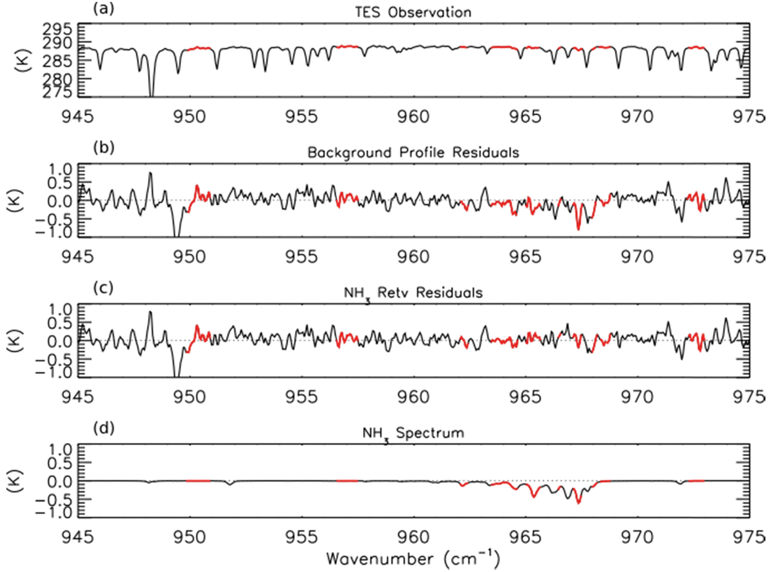
NH3 retrievals were performed using TES Level 1B spectra (V003) [41] following the method of Shephard et al. [20], which has been implemented in V005 of the TES Level 2 products. The a priori profiles and covariance matrices for TES NH3 retrievals are derived from GEOS-Chem model simulations of the 2005 global distribution of NH3. Figure 1a shows an observed TES brightness temperature spectrum in the region of strong NH3 absorption for a scan of a fresh Canadian smoke plume. Figures 1b,c show the brightness temperature residuals (observed spectrum minus modeled spectrum) for the unpolluted background NH3 profile and the retrieved NH3 profile, respectively, while Figure 1d shows the modeled spectrum of NH3, calculated as the difference between the modeled spectrum including the retrieved NH3 profile and the modeled spectrum without any NH3. We can see a strong residual (−0.8 K) in the background profile spectrum that is substantially reduced following retrieval of NH3. (The second strong residual feature near 949 cm−1 in panels b and c appears to be due to the ν7 Q-branch of ethylene (C2H4), as is discussed in Section 3.4 below.)
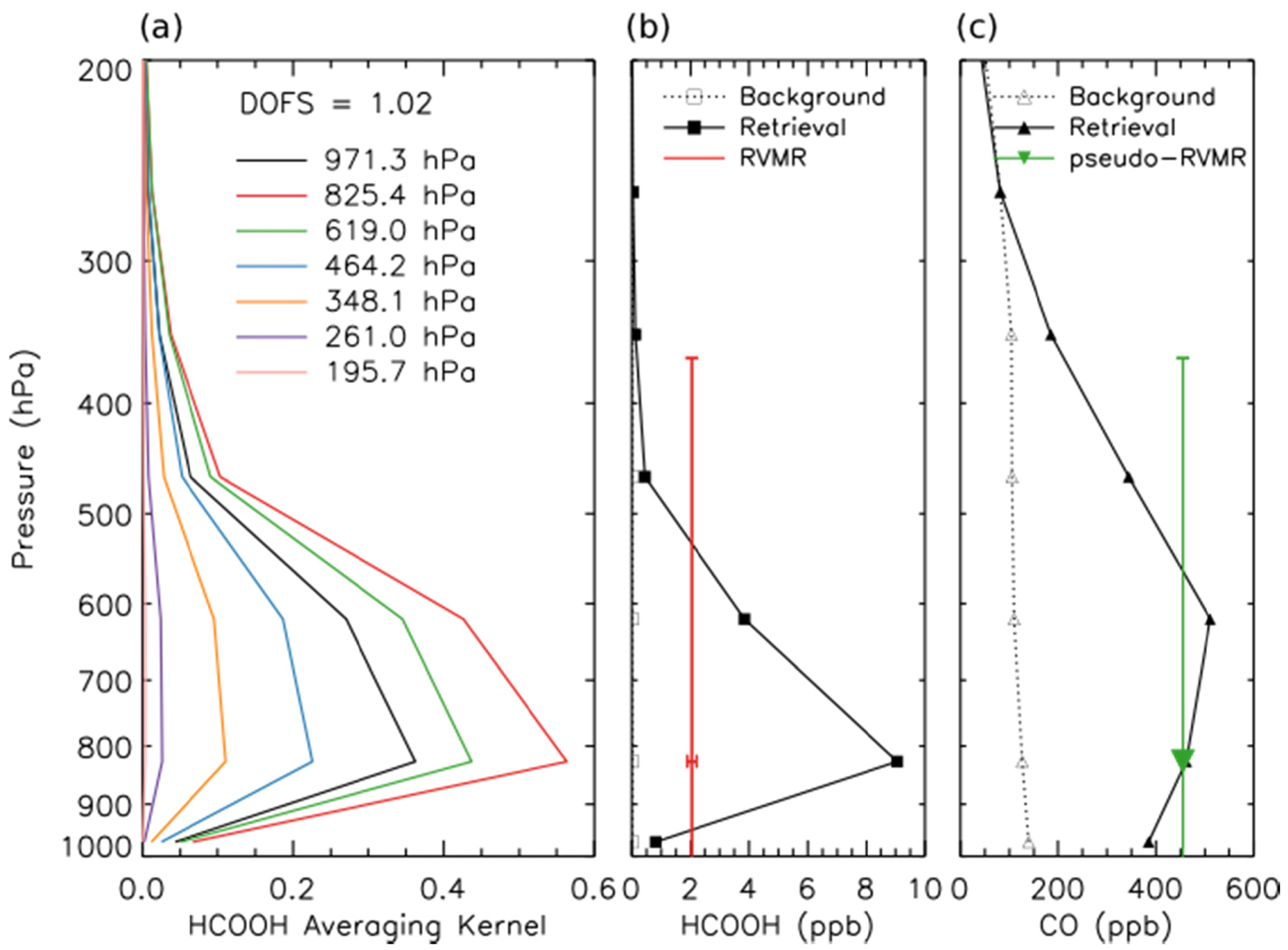
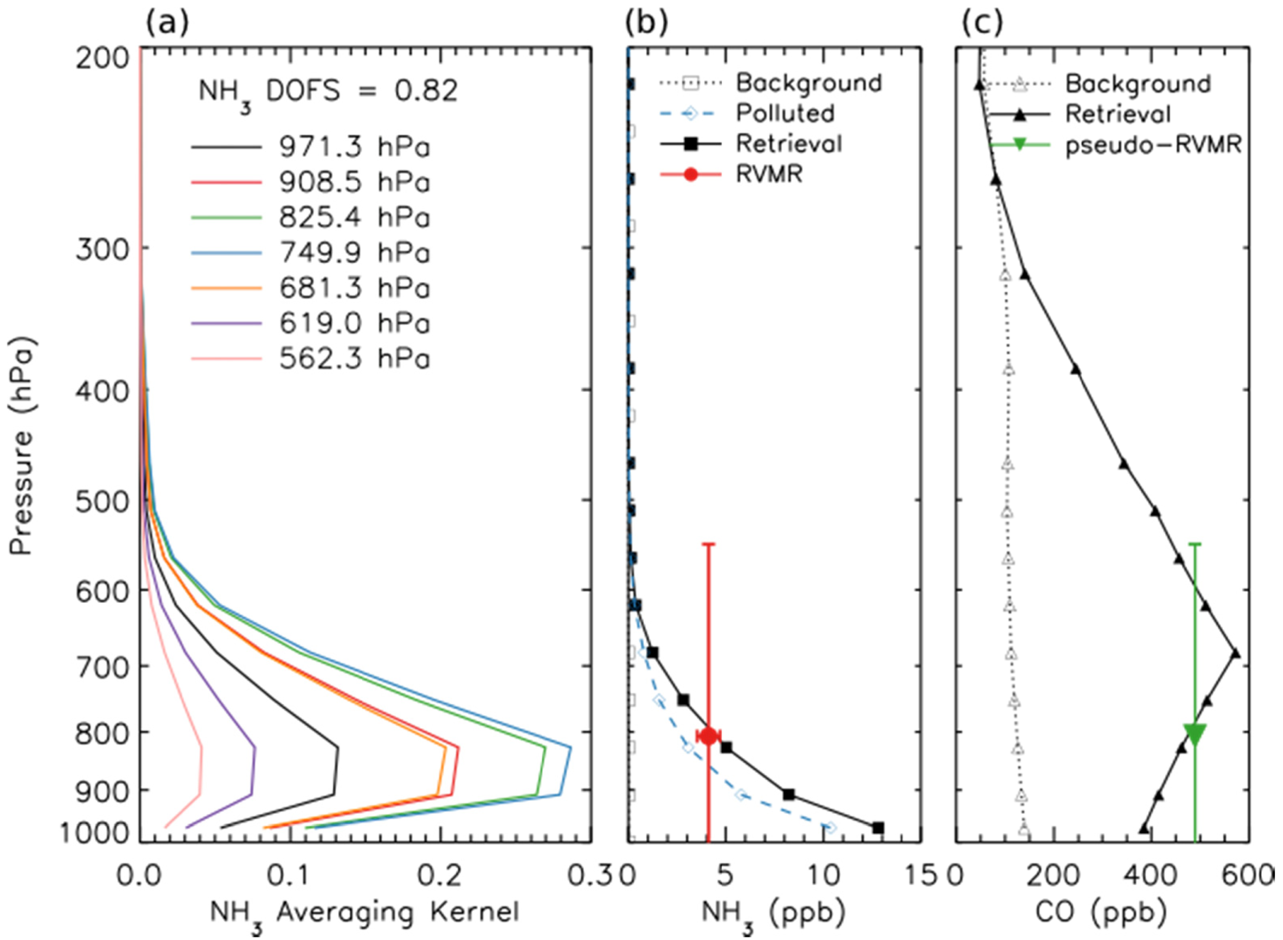
Figure 2a shows the averaging kernel for the same NH3 retrieval. The retrievals are performed using 14 vertical levels. However, the number of DOFS is generally not greater than one, meaning that it is not possible to obtain information about the shape of the profile from these retrievals. In order to minimize the influence of the a priori constraints on the end result, it is desirable to report one retrieved quantity per DOFS. However, performing a “profile” retrieval offers a major advantage in that us allows the calculation of diagnostics, such as the averaging kernels, that enable characterization of the spatial and temporal variability of the vertical sensitivity of the measurements. Therefore, for this work, the retrievals are performed on 14 levels in order to take advantage of the sensitivity characterization that this enables, then post-processed to calculate a single quantity that better represents the information that is really available in the measurement and that is relatively insensitive to the a priori constraints. Shephard et al. developed a Representative Volume Mixing Ratio (RVMR) metric for NH3 [20] based on similar techniques used previously for CH4 [51] and CH3OH [19]. This RVMR represents a TES sensitivity weighted average value where the influence of the a priori profile is reduced as much as possible. (Note that for NH3, one of three a priori profiles is selected based on the signal-to-noise ratio in the TES NH3 band [20]. For the scan shown in Figures 1 and 2, the polluted a priori, shown as a dashed blue line in Figure 2b, was selected.) Figure 2b shows a retrieved profile of NH3 for a fresh Canadian smoke plume as a solid black line, while the red circle is the RVMR calculated from the profile. The horizontal error bars show the uncertainty in the RVMR due to noise in the TES spectrum, while the vertical bars encompass the region of TES sensitivity to NH3, defined as the full width at half maximum (FWHM) of the averaging kernel at the pressure level of the RVMR [20]. With the a priori assumption about profile shape that was chosen here the NH3 RVMR is roughly 20% to 60% of the retrieved surface value for NH3. The estimated minimum detection level is an RVMR of approximately 0.3 ppb, corresponding to a profile with a surface mixing ratio of about 1–2 ppb [20]. However, it must be noted that this is merely a general estimate of the minimum detection level, which depends strongly on the location of peak NH3 mixing ratio and the thermal structure of the atmosphere for a given scan [20], and thus retrieved NH3 RVMRs of less than 0.3 ppb are considered valid and are included in our analysis.
The excess mixing ratio of a trace gas like NH3 (EMR, ΔNH3) is defined as the mixing ratio of the gas in the smoke plume minus its mixing ratio in the background. This excess mixing ratio can be normalized using the excess mixing ratio of CO to give the normalized excess mixing ratio (NEMR, ΔNH3/ΔCO). The emission ratio (ER) is a special case of the NEMR where the measurements are made in fresh smoke near the fire source [3]. The NEMR of a trace gas can be highly variable for reactive gases downwind of fires due to the different rates of deposition and secondary photochemical production and loss for the trace gas and CO. In this paper, we will refer to our derived NEMRs for fresh Canadian smoke observed by TES as emission ratios; however, these emission ratios are inherently convolutions of the initial NEMR and any secondary production and loss processes that have taken place within the smoke plume during plume lofting and transport from the fire source [28]. Furthermore, the lower sensitivity of the TES retrievals near the surface (see Figure 2a) means that TES will preferentially sample smoke from the flaming stages of combustion, as these emissions are more likely to be lofted well above the surface. This lower sensitivity near the surface is due to the physics of nadir thermal infrared sounding: when the surface and the layers of the atmosphere near the surface have similar temperatures (low thermal contrast), we cannot distinguish between radiation emitted by the surface and radiation emitted by the lowest layers of the atmosphere. Similar caution must be used in interpreting emission ratios measured from other platforms: for example, NEMRs of NH3 measured at the ground are generally much higher than those measured by aircraft, as the aircraft does not sample the emissions from residual smoldering combustion very close to the ground (see Section 3.1 below).
In order to use the TES retrievals of NH3 and CO to calculate the emission ratio of NH3, we first calculated the RVMR for NH3 following the procedure of Shephard et al. [20]. Since the DOFS for the CO retrieval are generally higher than for NH3, in order to obtain a comparable metric we transform the TES CO retrieval using the same grid and weightings as were used to generate the NH3 RVMR to obtain a pseudo-RVMR for CO. Figure 2c shows the retrieved CO profile for a fresh Canadian smoke plume as a solid black line while the pseudo-RVMR for CO is shown in green. The emission ratio of NH3 was then calculated as the slope of a least squares linear regression of the NH3 RVMR and the CO pseudo-RVMR.
2.3. HCOOH Retrieval
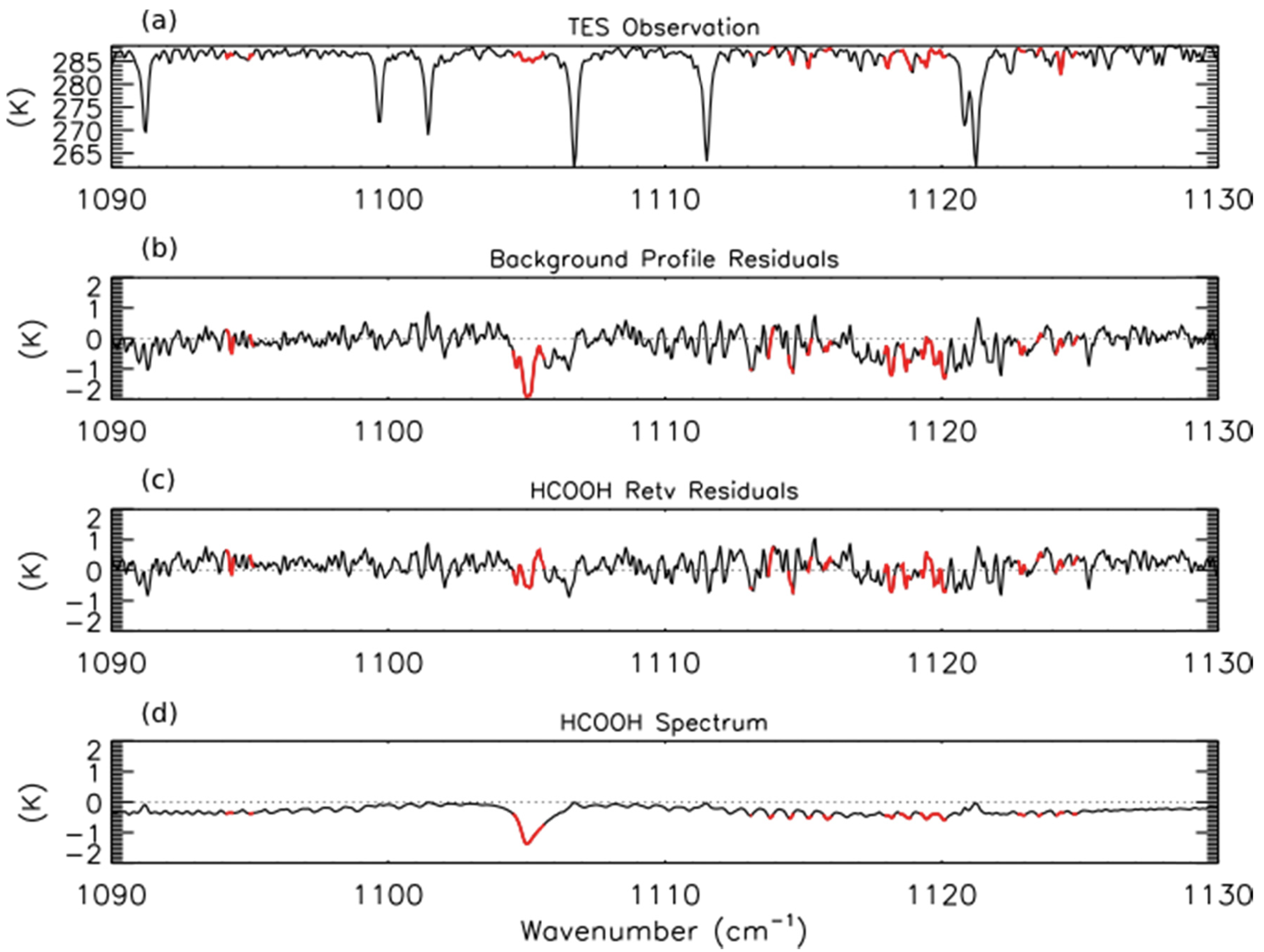
We have developed a prototype retrieval for formic acid (HCOOH) from TES Level 1B spectra. The retrieval approach is similar to that used for NH3. The spectroscopic parameters for HCOOH were taken from the HITRAN 2008 database, which substantially improved the estimates of the strengths of HCOOH lines by removing interference from the formic acid dimer [52]. All other spectroscopic parameters were taken from v1.4 of the TES spectroscopic line parameters [53]. The a priori constraint and covariance matrix were compiled from GEOS-Chem model simulations of the 2004 global background mixing ratios of HCOOH; however, these background profiles may be biased low, as GEOS-Chem tends to underestimate HCOOH in the northern mid-latitudes [28]. For HCOOH, the initial guess profile is the same as the a priori constraint vector. LBLRTM was run using TES Level 2 (V004) retrievals of temperature, average cloud optical depth, emissivity, reflectivity, H2O, CO, O3, and CH4. Profiles of CO2 and N2O were taken from the TES Level 2 supplemental data files. The top panel of Figure 3 shows the observed TES brightness temperature spectrum between 1090–1130 cm−1 for a scan of fresh smoke from a Canadian fire with the HCOOH retrieval microwindows shown in red. Note that only some sections of the HCOOH band have been retained in order to remove interfering lines from other species, principally water vapor. The second panel shows the residuals (observed spectrum minus modeled spectrum) for the background HCOOH profile. We see a strong (−2 K) residual in the HCOOH Q-branch (∼1105 cm−1), which is removed after retrieval of HCOOH as seen in the third panel of Figure 3.
An RVMR for HCOOH and a corresponding CO pseudo-RVMR were calculated following the procedure of Shephard et al. for NH3 [20], as illustrated in Figure 4. The RVMR for HCOOH is lower than the retrieved value at the level of maximum sensitivity to HCOOH, poissibly because the TES sensitivity to HCOOH covers a wide pressure range. The emission ratio of HCOOH was calculated as the slope of the least squares linear regression of the HCOOH RVMR and the CO pseudo-RVMR.
2.4. Detection of PAN and C2H4
In order to use TES to detect PAN in boreal smoke plumes, we calculated the differences (residuals) between the TES Level 1B spectra (V003) and a forward run of LBLRTM using v1.4 of the TES spectroscopic line parameters for the region of strong absorption by PAN (1140–1180 cm−1). As for the retrievals of HCOOH, the model was run using TES Level 2 (V004) retrievals of temperature, emissivity, reflectivity, average cloud optical depth, H2O, CO, O3, and CH4 and profiles of CO2 and N2O were taken from the TES Level 2 supplemental data files. Preliminary model runs using the spectrally resolved effective cloud optical depth retrieved by TES led to unphysical slopes in the residuals versus wavenumber between 1100 and 1200 cm−1. We removed these slopes by setting cloud optical depth in this spectral region to the average effective cloud optical depth included in the TES Level 2 products; however, the spectral signature of PAN was detectable regardless of which TES cloud product was used. The absorption cross section of PAN was taken from HITRAN 2008 [52].
A similar procedure was used to detect C2H4 in TES spectra, with the addition that the surface emissivity, surface temperature, and NH3 profile were taken from the final results of the NH3 retrieval described in Section 2.2 above. The line parameters for C2H4 were taken from v1.4 of the TES spectroscopic line parameters.
3. Results and Discussion
3.1. Emission Ratio of NH3
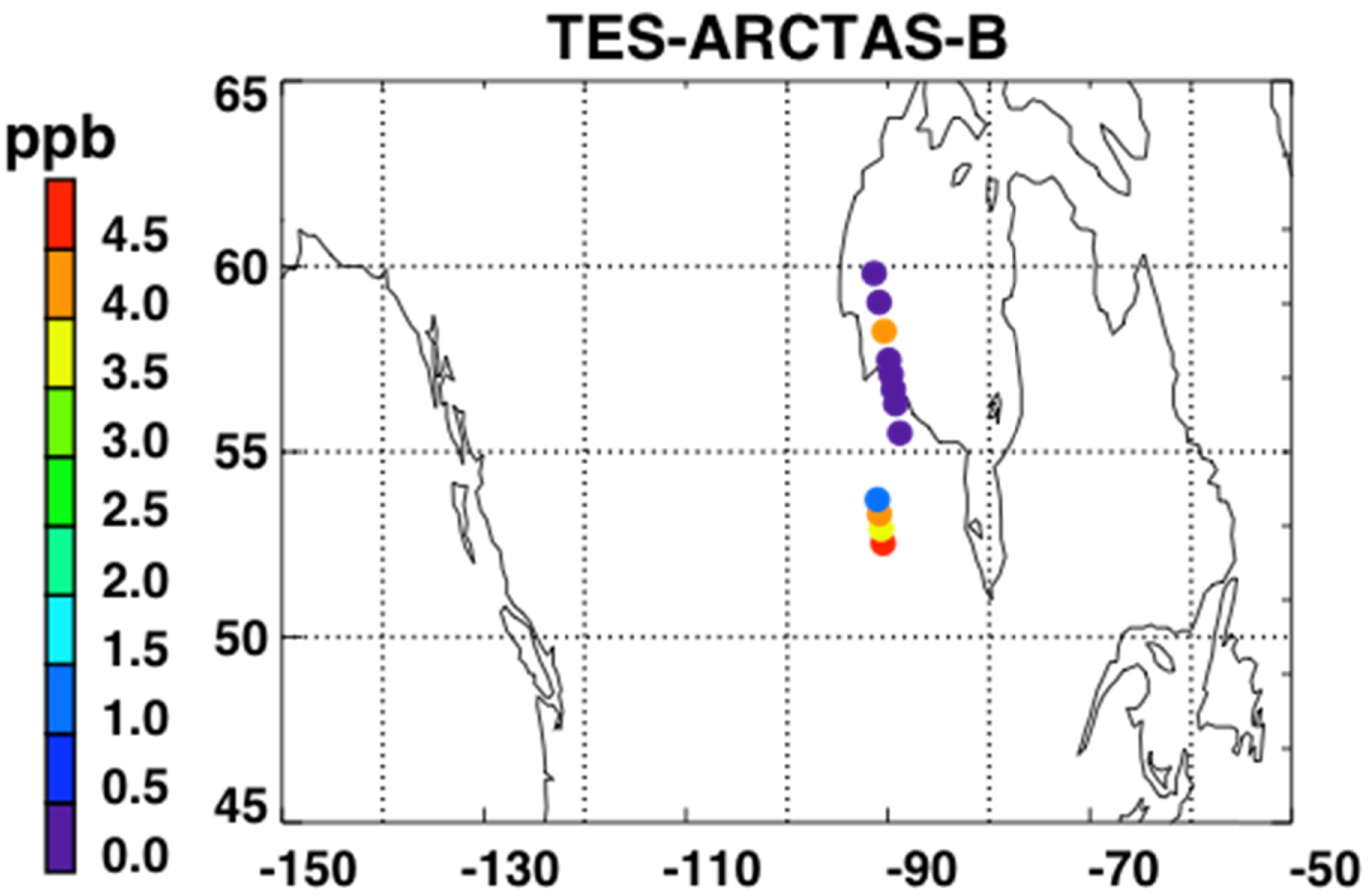
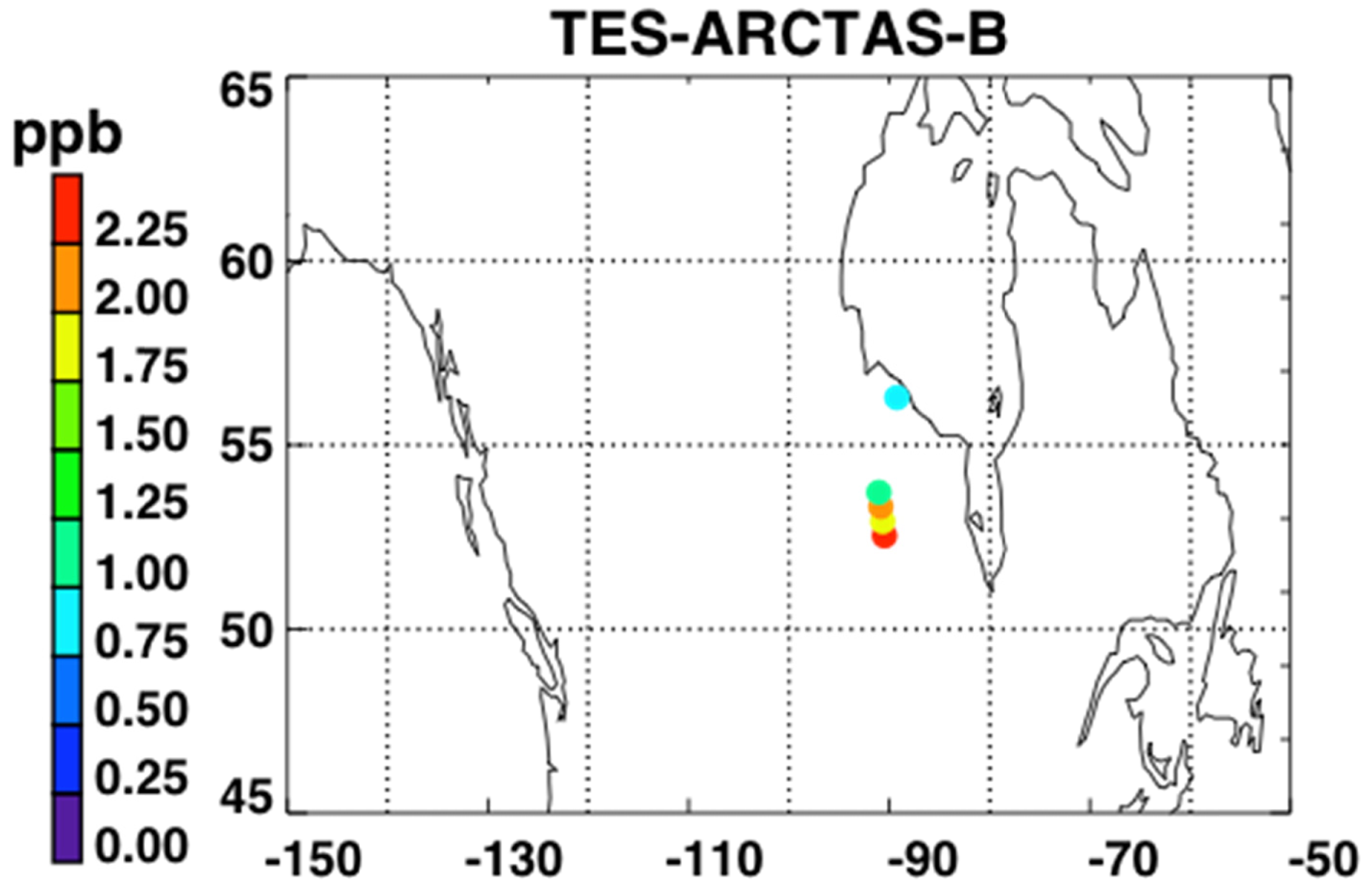
Figure 5 shows a map of the retrieved NH3 RVMR values within smoke plumes from Canadian biomass burning in the summer of 2008. We have filtered the retrievals for quality following Shephard et al. [20]. First, NH3 retrievals are rejected if the DOFS are less than 0.1 or if the average cloud optical depth is greater than 1. Second, retrievals with DOFS less than 0.5 are rejected if the thermal contrast between the surface and the atmospheric layer nearest the surface is between −7 K and 10 K.
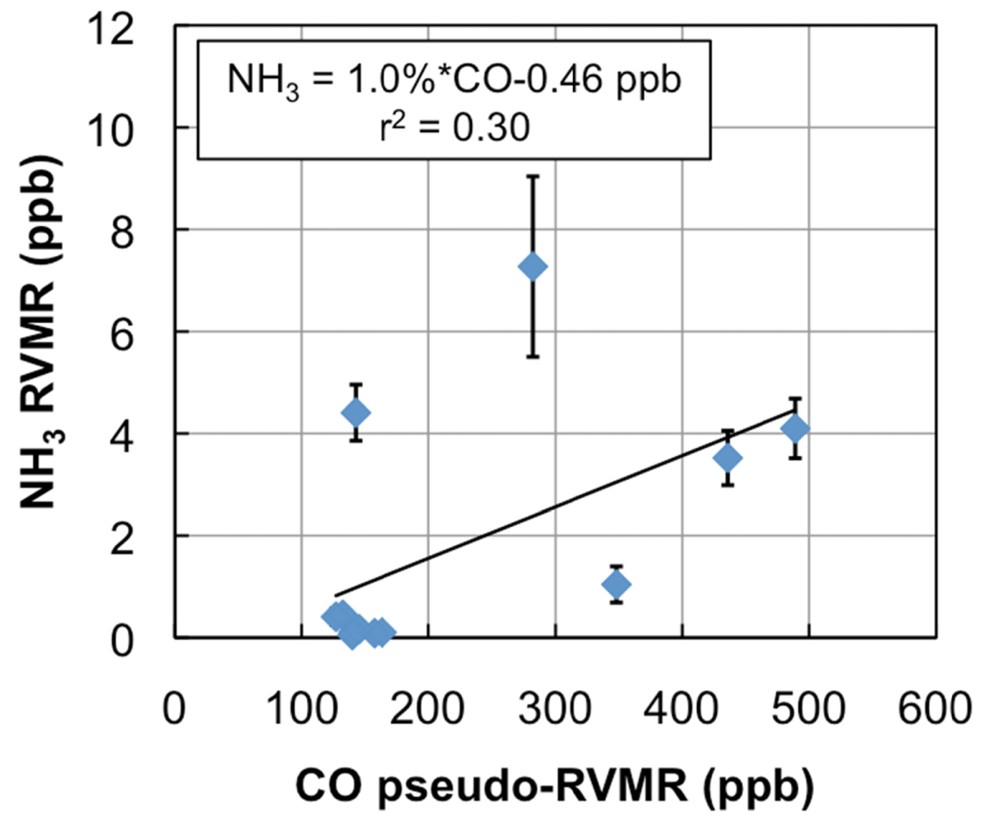
Figure 6 shows the NH3 RVMR versus the CO pseudo-RVMR for all of the retrievals shown on the map in Figure 5. The most elevated amounts of CO and NH3 come from a fresh smoke plume from a single Canadian fire observed by TES between 52.5–54.1°N and 90.5–91.8°W at 19:03 UTC on 1 July 2008 (TES Run #7656). Due to the high retrieved values for CO (>500 ppb), this plume likely contains concentrated fresh smoke. Also included are retrievals of NH3 within a more dilute smoke plume observed between 55.5–59.8°N and 88.8–91.4°W at 18:51 UTC on 17 June 2008 (TES Run #7472).
We calculate the NH3 emission ratio (ΔNH3/ΔCO) for these fires as 1.0% ± 0.5%. However, there is a large amount of scatter in this plot, which leads to a low correlation between CO and NH3 (r2 = 0.30). The scatter is likely due to the combination of: (1) variations in plume heights, which change the relative sensitivity of TES to CO and NH3 in the smoke plume; (2) variations in the age of the smoke plumes, as older plumes could have lost more NH3 to chemical reaction or deposition, and (3) variations in the initial emissions of ammonia from the fires, which are in turn related to differences in the relative fraction of flaming versus smoldering combustion as well as variations in fuel nitrogen content.
Table 1 compares our derived emission ratio for NH3 to previous satellite, aircraft, and ground measurements of ammonia emission ratios for boreal biomass burning. Our value is close to the value of 1.3% derived from IASI retrievals in Siberian smoke over East Mongolia [9]. The results from the aircraft and ground studies are substantially different with ground studies showing values of ΔNH3/ΔCO that are a factor of 5 higher than the aircraft or satellite studies. The higher ground values are likely due to emissions of NH3 from residual smoldering combustion very close to the ground [3] where aircraft cannot sample and satellites have little sensitivity to NH3 (see Figure 2). Thus, both aircraft and satellites are likely to underestimate the true emissions of NH3 from biomass burning fires unless the emission factors from aircraft and satellite studies are carefully combined with ground observations, such as in the review of Akagi et al. [3]. In addition, given the discrepancy between aircraft and ground observations, nadir-viewing satellite observations of NH3 are most appropriately compared with aircraft observations, as satellites will not be very sensitive to the ground-level residual smoldering emissions detected in ground studies. Our NH3 emission factor of 1.0% ± 0.5% is similar to the values of 1.3% ± 0.7% and 1.7% ± 0.9% reported for Alaskan forest fires in the aircraft studies of Nance et al. [54] and Goode et al. [55], respectively, but is substantially higher than the value of 0.16% ± 0.14% reported by Radke et al. for boreal forests [56]. Furthermore, our value lies within the uncertainty range of the average value of 1.0% ± 0.7% (boreal forests, aircraft studies only) reported in the review of Akagi et al. [3], as well as the value of 2.6% ± 2.2% (all extratropical forests, all study types) in the review of Andreae and Merlet [57].
3.2. Emission Ratio of HCOOH
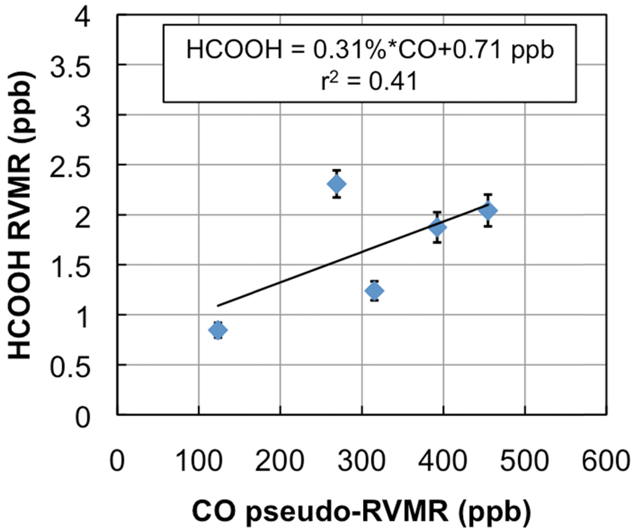
Figure 7 shows a map of the retrieved HCOOH RVMR values within smoke plumes from boreal biomass burning over Canada. We have removed retrievals with less than 0.5 DOFS for HCOOH, which also eliminated retrievals with an HCOOH RVMR of less than 0.5 ppbv. The smoke plumes included in the analysis are the same as described above for NH3. Figure 8 shows the HCOOH RVMR versus the CO pseudo-RVMR for all of the retrievals shown on the map in Figure 7. We calculate the emission ratio ΔHCOOH/ΔCO for these fires as 0.31% ± 0.21%. As we saw for NH3, there is a large amount of scatter in this plot that leads to a low correlation between CO and HCOOH (r2 = 0.41). As discussed above, this scatter is likely due to the combination of variations in (1) plume heights, (2) plume ages, and (3) initial smoke emissions of HCOOH. The large pressure range of TES sensitivity to HCOOH may also contribute to the low correlation of HCOOH with CO. It is worth noting that the ACE-FTS observations of HCOOH within boreal biomass burning plumes showed a much higher r2 value (0.86), likely due to the fact that the higher vertical resolution of limb retrievals means that ACE is better able to separate the different vertical layers of the plume which are averaged together by nadir-viewing sounders like TES and IASI [31].
Table 2 compares our derived emission ratio for HCOOH to previous satellite, aircraft, and ground measurements of formic acid emission ratios for boreal biomass burning. Our HCOOH emission ratio is slightly lower than the ratio of 0.38% ± 0.06% derived from ACE-FTS observations [31], possibly due to the fact that a limb-sounder like ACE is more sensitive to plumes that reach high altitudes; this type of plume is more common over more flaming fires since fire power output peaks during flaming combustion [4]. Table 2 shows that our value is similar to the emission ratios for HCOOH derived from aircraft and ground studies, with the exception of the value of 3.7% ± 2.0% reported for Canadian forests by Lefer et al. [60], which is about a factor of 10 higher than the average value for boreal biomass burning in the review of Akagi et al. [3]. However, Lefer et al. note that the elevated enhancement ratios of HCOOH they observed (0.82% to 6.2%) are likely due to HCOOH production within the plumes in the first couple hours after emission, and do not necessarily reflect the initial emissions. When the Lefer et al. study is removed, the Andreae and Merlet average becomes 0.85% ± 0.53%, with the relatively higher value of HCOOH likely due to the inclusion of midlatitude fires as well as boreal fires in the average [57].
3.3. Detection of PAN
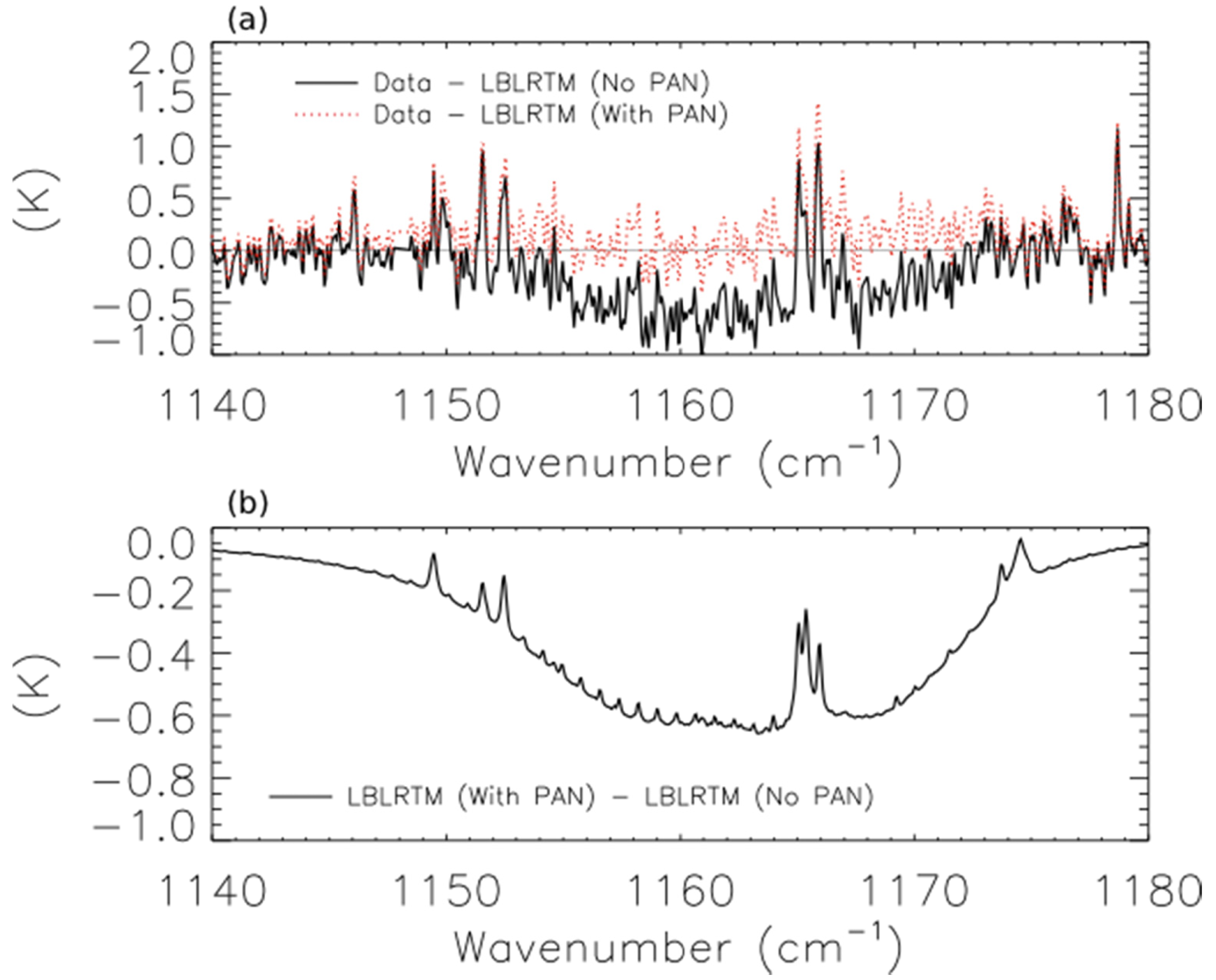
The solid black line of Figure 9a shows the brightness temperature residuals (data minus model) for the scan of fresh smoke from a Canadian fire at 53.32°N and 90.84°W.
The two lobes of PAN absorption are clearly visible on either side of the water line at ∼1165 cm−1. The dotted red line shows the residuals when a hypothetical PAN profile with a peak concentration of 1.9 ppb at 560 hPa is added to the forward model, and Figure 9b shows the modeled PAN spectrum as a solid black line. Adding the PAN profile substantially reduces the mean residuals, but this peak concentration of PAN in the assumed profile is about a factor of 2 higher than the concentration of PAN observed 30–60 min downwind of the Lake McKay fire in Saskatchewan, Canada during ARCTAS-B [12]. We have also detected PAN in a scan of aged smoke from Siberian biomass burning observed near Kamchatka (not shown). These two scans shared several common features, including relatively high mixing ratios of CO (mixing ratio > 250 ppbv at 510 hPa) and low average cloud optical depth (<0.1). This low cloud optical depth may be a necessary but insufficient criterion for detecting PAN in biomass burning smoke plumes with TES.
3.4. Detection of C2H4
As mentioned in Section 2.2 above, there is a second strong residual feature in Figure 1c near 949 cm−1 that appears to be due to absorption by C2H4.
Figure 10b shows this residual feature, which partially overlaps with the strong CO2 line [39] that is visible in the TES spectrum shown in Figure 10a. Figure 10c shows that the addition of a hypothetical C2H4 profile to the model (with a peak concentration of 1.9 ppb at the surface) removes this feature. This peak C2H4 mixing ratio is approximately the 85th percentile of C2H4 observations observed downwind of the Lake McKay fire in Saskatchewan, Canada during ARCTAS-B [12]. While the scan in Figure 10 did have a low cloud optical depth, this criterion is likely to be less important for detecting C2H4 within fresh biomass burning plumes using TES, as the residual feature of C2H4 is both stronger and sharper than the PAN feature. However, the short lifetime of C2H4 may make it difficult to detect in smoke that is several hours old.
4. Conclusions
We have retrieved mixing ratios of ammonia (NH3) and formic acid (HCOOH) within biomass burning smoke plumes over Canada from TES radiance measurements. We have combined these retrievals with the TES retrievals of CO to calculate molar ratios of NH3 and HCOOH to CO within biomass burning plumes by calculating representative volume mixing ratios for NH3 and HCOOH and then mapping the CO retrieval to the same vertical grid. Our estimated emission ratios for NH3 (1.0% ± 0.5%) and HCOOH (0.31% ± 0.21%) for forest fires in Canada are within the range of values reported in the literature for airborne and satellite studies of boreal biomass burning emissions. This work thus provides a method for the use of TES spectra to study the emissions of NH3 and HCOOH from biomass burning. This method, if applied to the entire TES data set, would help to estimate the spatial and temporal variability of these emissions. This information could then be used, in concert with the other satellite observations discussed in Section 1 of our manuscript, to provide improved estimates of the emissions of these trace gases for use in models of atmospheric chemistry, air quality, and climate.
We have shown that TES can observe peroxy acetyl nitrate (PAN) and ethylene (C2H4) within boreal biomass burning plumes. A low cloud optical depth (<0.1) appears to be required for successful detection of PAN by TES within biomass burning smoke plumes. Continuing this line of research could lead to maps of tropospheric PAN concentrations near source regions, which would help to constrain the fate of NOx emission within atmospheric chemistry models. These could be combined with satellite estimates of the emissions of ethylene from biomass burning to help reduce the uncertainty in the impact of biomass burning on tropospheric ozone.


| ΔNH3/ΔCO | Ecosystem/Fuel | Study Type | Source |
|---|---|---|---|
| 1.0% ± 0.5% | Canadian Forest | Satellite (TES) | This Study |
| 1.3% | Siberian Forest | Satellite (IASI) | [9] |
| 0.16% ± 0.14% | Boreal Forests | Aircraft | [56] |
| 1.3% ± 0.7% | Alaskan Forest | Aircraft | [54] |
| 1.7% ± 0.9% | Alaskan Forest | Aircraft | [55] |
| 6.9% ± 11.1% | Boreal Peat | Ground | [58] |
| 5.9% ± 3.6% | Boreal organic soil | Ground | [58] |
| 6.9% ± 3.2% | Boreal organic soil | Ground | [59] |
| 1.7% ± 2.2% | Boreal dead, woody material | Ground | [59] |
| 3.5% | Alaskan Duff | Laboratory | [4] |
| 1.0% ± 0.7% | Boreal Forests | Review: Aircraft Only | [3] |
| 5.1% ± 5.6% | Boreal Forests | Review: Ground Only | [3] |
| 3.5% ± 3.2% | Boreal Forests | Review: Aircraft and Ground | [3] |
| 2.6% ± 2.2% | Extratropical Forests | Review: Aircraft, Satellite, and Ground | [57] |
| ΔHCOOH/ΔCO | Ecosystem/Fuel | Study Type | Source |
|---|---|---|---|
| 0.31% ± 0.21% | Canadian Forest | Satellite (TES) | This Study |
| 0.38% ± 0.06% | Canadian Forest | Satellite (ACE-FTS) | [31] |
| 0.31% ± 0.09% | Alaskan Forest | Aircraft | [55] |
| 0.26% ± 0.44% | Boreal Peat | Ground | [58] |
| 0.18% ± 0.12% | Boreal organic soil | Ground | [58] |
| 0.33% ± 0.29% | Boreal organic soil | Ground | [59] |
| 0.17% ± 0.18% | Boreal dead, woody material | Ground | [59] |
| 0.35% | Alaskan Duff | Laboratory | [4] |
| 0.28% ± 0.24% | Boreal Forests | Review, Aircraft and Ground | [3] |
| 3.7% ± 2.0% | Canadian Forest | Aircraft | [60] |
| 1.4% ± 1.4% | Extratropical Forests | Review, Aircraft, Satellite and Ground | [57] |
Acknowledgments
This research was supported by NASA grant NNX10AG65G to the University of Minnesota and NASA grants to Atmospheric and Environmental Research (AER) including Grant NNH08CD52C. This work was supported in part by the University of Minnesota Supercomputing Institute. We thank Eli Mlawer of AER, P. F. Bernath of the University of York, and the anonymous reviewers for their helpful comments.
References
- Crutzen, P.J.; Andreae, M.O. Biomass burning in the tropics: Impact on atmospheric chemistry and biogeochemical cycles. Science 1990, 250, 1669–1678. [Google Scholar]
- Bond, T.C.; Streets, D.G.; Yarber, K.F.; Nelson, S.M.; Woo, J.-H.; Klimont, Z. A technology-based global inventory of black and organic carbon emissions from combustion. J. Geophys. Res. 2004, 109. [Google Scholar] [CrossRef]
- Akagi, S.K.; Yokelson, R.J.; Wiedinmyer, C.; Alvarado, M.J.; Reid, J. S.; Karl, T.; Crounse, J.D.; Wennberg, P.O. Emission factors for open and domestic biomass burning for use in atmospheric models. Atmos. Chem. Phys. 2011, 11, 4039–4072. [Google Scholar]
- Burling, I.R.; Yokelson, R.J.; Griffith, D.W.T.; Johnson, T.J.; Veres, P.; Roberts, J.M.; Warneke, C.; Urbanski, S.P.; Reardon, J.; Weise, D.R.; et al. Laboratory measurements of trace gas emissions from biomass burning of fuel types from the southeastern and southwestern United States. Atmos. Chem. Phys. 2010, 10, 11115–11130. [Google Scholar]
- Wooster, M.J.; Roberts, G.; Perry, G.L.W.; Kaufman, Y.J. Retrieval of biomass combustion rates and totals from fire radiative power observations: FRP derivation and calibration relationships between biomass consumption and fire radiative energy release. J. Geophys. Res. 2005, 110. [Google Scholar] [CrossRef]
- Ichoku, C.; Kaufman, Y.J. A method to derive smoke emission rates from MODIS fire radiative energy measurements. IEEE Trans. Geosci. Rem. Sensing 2005, 43, 2636–2649. [Google Scholar]
- Mebust, A.K.; Russell, A.R.; Hudman, R.C.; Valin, L.C.; Cohen, R.C. Characterization of wildfire NOx emissions using MODIS fire radiative power and OMI tropospheric NO2 columns. Atmos. Chem. Phys. 2011, 11, 5839–5851. [Google Scholar]
- Kopacz, M.; Jacob, D.J.; Fisher, J.A.; Logan, J.A.; Zhang, L.; Megretskaia, I.A.; Yantosca, R.M.; Singh, K.; Henze, D.K.; Burrows, J.P.; et al. Global estimates of CO sources with high resolution by adjoint inversion of multiple satellite datasets (MOPITT, AIRS, SCIAMACHY, TES). Atmos. Chem. Phys. 2010, 10, 855–876. [Google Scholar]
- Coheur, P.-F.; Clarisse, L.; Turquety, S.; Hurtmans, D.; Clerbaux, C. IASI measurements of reactive trace species in biomass burning plumes. Atmos. Chem. Phys. 2009, 9, 5655–5667. [Google Scholar]
- Clarisse, L.; R'Honi, Y.; Coheur, P.-F.; Hurtmans, D.; Clerbaux, C. Thermal infrared nadir observations of 24 atmospheric gases. Geophys. Res. Lett. 2011, 38. [Google Scholar] [CrossRef]
- Verma, S.; Worden, J.; Pierce, B.; Jones, D.B.A.; Al-Saadi, J.; Boersma, F.; Bowman, K.; Eldering, A.; Fisher, B.; Jourdain, L.; et al. Ozone production in boreal fire smoke plumes using observations from the Tropospheric Emission Spectrometer and the Ozone Monitoring Instrument. J. Geophys. Res. 2009, 114. [Google Scholar] [CrossRef]
- Alvarado, M.J.; Logan, J.A.; Mao, J.; Apel, E.; Riemer, D.; Blake, D.; Cohen, R.C.; Min, K.-E.; Perring, A.E.; Browne, E.C.; et al. Nitrogen oxides and PAN in plumes from boreal fires during ARCTAS-B and their impact on ozone: An integrated analysis of aircraft and satellite observations. Atmos. Chem. Phys. 2010, 10, 9739–9760. [Google Scholar]
- Dupont, R.; Pierce, B.; Worden, J.; Hair, J.; Fenn, M.; Hamer, P.; Natarajan, M.; Schaack, T.; Lenzen, A.; Apel, E.; et al. Reconstructing ozone chemistry from Asian wild fires using models, satellite and aircraft measurements during the ARCTAS campaign. Atmos. Chem. Phys. Discuss. 2010, 10, 26751–26812. [Google Scholar]
- Jacob, D.J.; Crawford, J.H.; Maring, H.; Clarke, A.D.; Dibb, J.E.; Emmons, L.K.; Ferrare, R.A.; Hostetler, C.A.; Russell, P.B.; Singh, H.B.; et al. The Arctic Research of the Composition of the Troposphere from Aircraft and Satellites (ARCTAS) mission: Design, execution, and first results. Atmos. Chem. Phys. 2010, 10, 5191–5212. [Google Scholar]
- Hegg, D.A.; Radke, L.F.; Hobbs, P.V.; Riggan, P.J. Ammonia emissions from biomass burning. Geophys. Res. Lett. 1988, 15, 335–337. [Google Scholar]
- Henze, D.K.; Seinfeld, J.H.; Shindell, D.T. Inverse modeling and mapping US air quality influences of inorganic PM2.5 precursor emissions using the adjoint of GEOS-Chem. Atmos. Chem. Phys. 2009, 9, 5877–5903. [Google Scholar]
- Langford, A.O.; Fehsenfeld, F.S.; Zachariassen, J.; Schimel, D.S. Gaseous ammonia fluxes and background concentrations in terrestrial ecosystems of the United States. Glob. Biogeochem. Cycles 1992, 6, 459–483. [Google Scholar]
- Worden, H.; Beer, R.; Rinsland, C. Airborne infrared spectroscopy of 1994 western wildfires. J. Geophys. Res. 1997, 102, 1287–1299. [Google Scholar]
- Beer, R.; Shephard, M.W.; Kulawik, S.S.; Clough, S.A.; Eldering, A.; Bowman, K.W.; Sander, S.P.; Fisher, B.M.; Payne, V.H.; Luo, M.; et al. First satellite observations of lower tropospheric ammonia and methanol. Geophys. Res. Lett. 2008, 35. [Google Scholar] [CrossRef]
- Shephard, M.W.; Cady-Pereira, K.E.; Luo, M.; Henze, D.K.; Pinder, R.W.; Walker, J.T.; Rinsland, C.P.; Bash, J.O.; Zhu, L.; Payne, V.H.; et al. TES ammonia retrieval strategy and global observations of the spatial and seasonal variability of ammonia. Atmos. Chem. Phys. Discuss. 2011, 11, 16023–16074. [Google Scholar]
- Pinder, R.W.; Walker, J.T.; Bash, J.O.; Cady-Pereira, K.E.; Henze, D.K.; Luo, M.; Osterman, G.B.; Shephard, M.W. Quantifying spatial and seasonal variability in atmospheric ammonia with in situ and space-based observations. Geophys. Res. Lett. 2011, 38. [Google Scholar] [CrossRef]
- Clarisse, L.; Clerbaux, C.; Dentener, F.; Hurtsmans, D.; Coheur, P.-F. Global ammonia distribution derived from infrared satellite observations. Nat. Geosci. 2009, 2, 479–483. [Google Scholar]
- Kawamura, K.; Steinberg, S.; Kaplan, I.R. Homologous series of C1-C10 monocarboxylic acids and C1-C6 carbonyls in Los Angeles air and motor vehicle exhausts. Atmos. Environ. 2000, 34, 4175–4191. [Google Scholar]
- Keene, W.C.; Galloway, J.N. The biogeochemical cycling of formic and acetic acids through the troposphere: An overview of current understanding. Tellus B 1988, 40B, 322–334. [Google Scholar]
- Avery, G.B, Jr.; Tang, Y.; Kieber, R.J.; Willey, J.D. Impact of recent urbanization on formic and acetic acid concentrations in coastal North Carolina rainwater. Atmos. Environ. 2001, 35, 3353–3359. [Google Scholar]
- Shephard, M.W.; Goldman, A.; Clough, S.A.; Mlawer, E.J. Spectroscopic improvements providing evidence of formic acid in AERI-LBLRTM validation spectra. J. Quant. Spectrosc. Radiat. Transf. 2003, 82, 383–390. [Google Scholar]
- Rinsland, C.P.; Mahieu, E.; Zander, R.; Goldman, A.; Wood, S.; Chiou, L. Free tropospheric measurements of formic acid (HCOOH) from infrared ground-based solar absorption spectra: Retrieval approach, evidence for a seasonal cycle, and comparison with model calculations. J. Geophys. Res. 2004, 109. [Google Scholar] [CrossRef]
- Paulot, F.; Wunch, D.; Crounse, J.D.; Toon, G.C.; Millet, D.B.; DeCarlo, P.F.; Vigouroux, C.; Deutscher, N.M.; González Abad, G.; Notholt, J.; et al. Importance of secondary sources in the atmospheric budgets of formic and acetic acids. Atmos. Chem. Phys. 2011, 11, 1989–2013. [Google Scholar]
- Yokelson, R.J.; Crounse, J.D.; DeCarlo, P.F.; Karl, T.; Urbanski, S.; Atlas, E.; Campos, T.; Shinozuka, Y.; Kapustin, V.; Clarke, A.D.; et al. Emissions from biomass burning in the Yucatan. Atmos. Chem. Phys. 2009, 9, 5785–5812. [Google Scholar]
- Rinsland, C.P.; Boone, C.D.; Bernath, P.F.; Mahieu, E.; Zander, R.; Dufour, G.; Clerbaux, C.; Turquety, S.; Chiou, L.; McConnell, J.C.; et al. First space-based observations of formic acid (HCOOH): Atmospheric Chemistry Experiment austral spring 2004 and 2005 Southern Hemisphere tropical-mid-latitude upper tropospheric measurements. Geophys. Res. Lett. 2006, 33. [Google Scholar] [CrossRef]
- Tereszchuk, K.A.; González Abad, G.; Clerbaux, C.; Hurtmans, D.; Coheur, P.-F.; Bernath, P.F. ACE-FTS measurements of trace species in the characterization of biomass burning plumes. Atmos. Chem. Phys. Discuss. 2011, 11, 16611–16637. [Google Scholar]
- Grutter, M.; Glatthor, N.; Stiller, G.P.; Fischer, H.; Grabowski, U.; Hopfner, M.; Kellmann, S.; Linden, A.; von Clarmann, T. Global distribution and variability of formic acid as observed by MIPAS-ENVISAT. J. Geophys. Res. 2010, 115. [Google Scholar] [CrossRef]
- Razavi, A.; Karagulian, F.; Clarisse, L.; Hurtmans, D.; Coheur, P.F.; Clerbaux, C.; Müller, J.F.; Stavrakou, T. Global distributions of methanol and formic acid retrieved for the first time from the IASI/MetOp thermal infrared sounder. Atmos. Chem. Phys. 2011, 11, 857–872. [Google Scholar]
- Val Martín, M.; Honrath, R.E.; Owen, R.C.; Pfister, G.; Fialho, P.; Barata, F. Significant enhancements of nitrogen oxides, black carbon, and ozone in the North Atlantic lower free troposphere resulting from North American boreal wildfires. J. Geophys. Res. 2006, 111. [Google Scholar] [CrossRef]
- Leung, F.-Y.T.; Logan, J.A.; Park, R.; Hyer, E.; Kasischke, E.; Streets, D.; Yurganov, L. Impacts of enhanced biomass burning in the boreal forests in 1998 on tropospheric chemistry and the sensitivity of model results to the injection height of emissions. J. Geophys. Res. 2007, 112. [Google Scholar] [CrossRef]
- Real, E.; Law, K.S.; Weinzierl, B.; Fiebig, M.; Petzold, A.; Wild, O.; Methven, J.; Arnold, S.; Stohl, A.; Huntrieser, H.; et al. Processes influencing ozone levels in Alaskan forest fire plumes during long-range transport over the North Atlantic. J. Geophys. Res. 2007, 112. [Google Scholar] [CrossRef]
- Jacob, D.; Wofsy, S.C.; Bakwin, P.S.; Fan, S.-M.; Harriss, R.C.; Talbot, R.W.; Bradshaw, J.D.; Sandholm, S.T.; Singh, H.B.; Browell, E.V.; et al. Summertime Photochemistry of the Troposphere at High Northern Latitudes. J. Geophys. Res. 1992, 97, 16421–16431. [Google Scholar]
- Moore, D.P.; Remedios, J.J. Seasonality of Peroxyacetyl nitrate (PAN) in the upper troposphere and lower stratosphere using the MIPAS-E instrument. Atmos. Chem. Phys. 2010, 10, 6117–6128. [Google Scholar]
- Coheur, P.-F.; Herbin, H.; Clerbaux, C.; Hurtmans, D.; Wespes, C.; Carleer, M.; Turquety, S.; Rinsland, C.P.; Remedios, J.; Hauglustaine, D.; et al. ACE-FTS observation of a young biomass burning plume: First reported measurements of C2H4, C3H6O, H2CO and PAN by infrared occultation from space. Atmos. Chem. Phys. 2007, 7, 5437–5446. [Google Scholar]
- Alvarado, M.J.; Prinn, R.G. Formation of ozone and growth of aerosols in young smoke plumes from biomass burning: 1. Lagrangian parcel studies. J. Geophys. Res. 2009, 114. [Google Scholar] [CrossRef]
- Shephard, M.W.; Worden, H.M.; Cady-Pereira, K.E.; Lampel, M.; Luo, M.; Bowman, K.W.; Sarkissian, E.; Beer, R.; Rider, D.M.; Tobin, D.C.; et al. Tropospheric Emission Spectrometer nadir spectral radiance comparisons. J. Geophys. Res. 2008, 113. [Google Scholar] [CrossRef]
- Clough, S.A.; Shephard, M.W.; Worden, J.; Brown, P.D.; Worden, H.M.; Luo, M.; Rodgers, C.D.; Rinsland, C.P.; Goldman, A.; Brown, L.; et al. Forward model and jacobians for tropospheric emission spectrometer retrievals. IEEE Trans. Geosci. Remote 2006, 44, 1308–1323. [Google Scholar]
- Shephard, M.W.; Clough, S.A.; Payne, V.H.; Smith, W.L; Kireev, S.; Cady-Pereira, K.E. Performance of the line-by-line radiative transfer model (LBLRTM) for temperature and species retrievals: IASI case studies from JAIVEx. Atmos. Chem. Phys. 2009, 9, 7397–7417. [Google Scholar]
- Rodgers, C.D. Inverse Methods for Atmospheric Sounding: Theory and Practice; World Scientific: Hackensack, NJ, USA, 2000. [Google Scholar]
- Bowman, K.W.; Rodgers, C.D.; Sund-Kulawik, S.; Worden, J.; Sarkissian, E.; Osterman, G.; Steck, T.; Luo, M.; Eldering, A.; Shephard, M.W.; et al. Tropospheric emission spectrometer: Retrieval method and error analysis. IEEE Trans. Geosci. Remote 2006, 44, 1297–1307. [Google Scholar]
- Kulawik, S.S.; Worden, J.; Eldering, A.; Bowman, K.; Gunson, M.; Osterman, G.B.; Zhang, L.; Clough, S.A.; Shephard, M.W.; Beer, R. Implementation of cloud retrievals for Tropospheric Emission Spectrometer (TES) atmospheric retrievals: Part 1. Description and characterization of errors on trace gas retrievals. J. Geophys. Res. 2006, 111. [Google Scholar] [CrossRef]
- Reid, J.S.; Koppmann, R.; Eck, T.F.; Eleuterio, D.P. A review of biomass burning emissions part II: Intensive physical properties of biomass burning particles. Atmos. Chem. Phys. 2005, 5, 799–825. [Google Scholar]
- Bowman, K.; Eldering, A.; Fisher, B.; Herman, R.; Jacob, D.; Jourdain, L.; Kulawik, S.; Luo, M.; Monarrez, R.; et al. Earth Observating System (EOS) Tropospheric Emission Spectrometer (TES) Level 2 (L2) Data User's Guide; Osterman, G., Ed.; Jet Propulsion Laboratory (JPL): Pasadena, CA, USA, 2008. [Google Scholar]
- Zhang, L.; Jacob, D.J.; Boersma, K.F.; Jaffe, D.A.; Olson, J.R.; Bowman, K.W.; Worden, J.R.; Thompson, A.M.; Avery, M.A.; Cohen, R.C.; et al. Transpacific transport of ozone pollution and the effect of recent Asian emission increases on air quality in North America: An integrated analysis using satellite, aircraft, ozonesonde, and surface observations. Atmos. Chem. Phys. 2008, 8, 6117–6136. [Google Scholar]
- Air Resources Laboratory. HYSPLIT—Hybrid Single Particle Lagrangian Integrated Trajectory Model. Available online: http://ready.arl.noaa.gov/HYSPLIT.php (accessed on 25 September 2008).
- Payne, V.H.; Clough, S.A.; Shephard, M.W.; Nassar, R.; Logan, J.A. Information-centered representation of retrievals with limited degrees of freedom for signal: Application to methane from the Tropospheric Emission Spectrometer. J. Geophys. Res. 2009, 17, 1095. [Google Scholar]
- Rothman, L.; Gordon, I.E.; Barbe, A.; Benner, D.C.; Bernath, P.F.; Birk, M.; Boudon, V.; Brown, L.R.; Campargue, A.; Champion, J.-P.; et al. The HITRAN 2008 molecular spectroscopic database. J. Quant. Spectrosc. Radiat. Transf. 2009, 110, 533–572. [Google Scholar]
- AER Line Parameter Database. What's New. Available online: http://rtweb.aer.com/line_param_frame.html (accessed on 1 August 2010).
- Nance, J.; Hobbs, P.; Radke, L.; Ward, D. Airborne measurements of gases and particles from an Alaskan wildfire. J. Geophys. Res. 1993, 98, 14873–14882. [Google Scholar]
- Goode, J.G.; Yokelson, R.J.; Ward, D.E.; Susott, R.A.; Babbitt, R.E.; Davies, M.A.; Hao, W.M. Measurements of excess O3, CO2, CO, CH4, C2H4, C2H2, HCN, NO, NH3, HCOOH, CH3COOH, HCHO and CH3OH in 1997 Alaskan biomass burning plumes by airborne fourier transform infraredspectrscopy (AFTIR). J. Geophys. Res. 2000, 105, 22147–22166. [Google Scholar]
- Radke, L.F.; Hegg, D.A.; Hobbs, P.V.; Nance, J.D.; Lyons, J.H.; Laursen, K.K.; Weiss, R.E.; Riggan, P.J.; Ward, D.E. Particulate and Trace Gas Emissions from Large Biomass Fires in North America. In Global Biomass Burning: Atmospheric, Climatic, and Biospheric Implications; Levine, J.S., Ed.; MIT Press: Cambridge, MA, USA, 1991; pp. 209–224. [Google Scholar]
- Andreae, M.; Merlet, P. Emission of trace gases and aerosols from biomass burning. Glob. Biogeochem. Cycles 2001, 15, 955–966. [Google Scholar]
- Yokelson, R.; Susott, R.; Ward, D.; Reardon, J.; Griffith, D. Emissions from smoldering combustion of biomass measured by open-path Fourier transform infrared spectroscopy. J. Geophys. Res. 1997, 102, 18865–18877. [Google Scholar]
- Bertschi, I.; Yokelson, R.J.; Ward, D.E.; Babbitt, R.E.; Susott, R.A.; Goode, J.G.; Hao, W.M. Trace gas and particle emissions from fires in large diameter and belowground biomass fuels. J. Geophys. Res. 2003, 108. [Google Scholar] [CrossRef]
- Lefer, B.; Talbot, R.W.; Harriss, R.H.; Bradshaw, J.D.; Sandholm, S.T.; Olson, J.O.; Sachse, G.W.; Collins, J.; Shipham, M.A.; Blake, D.R.; et al. Enhancement of acidic gases in biomass burning impacted air masses over Canada. J. Geophys. Res. 1994, 99, 1721–1737. [Google Scholar]
© 2011 by the authors; licensee MDPI, Basel, Switzerland. This article is an open access article distributed under the terms and conditions of the Creative Commons Attribution license (http://creativecommons.org/licenses/by/3.0/).
Share and Cite
Alvarado, M.J.; Cady-Pereira, K.E.; Xiao, Y.; Millet, D.B.; Payne, V.H. Emission Ratios for Ammonia and Formic Acid and Observations of Peroxy Acetyl Nitrate (PAN) and Ethylene in Biomass Burning Smoke as Seen by the Tropospheric Emission Spectrometer (TES). Atmosphere 2011, 2, 633-654. https://doi.org/10.3390/atmos2040633
Alvarado MJ, Cady-Pereira KE, Xiao Y, Millet DB, Payne VH. Emission Ratios for Ammonia and Formic Acid and Observations of Peroxy Acetyl Nitrate (PAN) and Ethylene in Biomass Burning Smoke as Seen by the Tropospheric Emission Spectrometer (TES). Atmosphere. 2011; 2(4):633-654. https://doi.org/10.3390/atmos2040633
Chicago/Turabian StyleAlvarado, Matthew J., Karen E. Cady-Pereira, Yaping Xiao, Dylan B. Millet, and Vivienne H. Payne. 2011. "Emission Ratios for Ammonia and Formic Acid and Observations of Peroxy Acetyl Nitrate (PAN) and Ethylene in Biomass Burning Smoke as Seen by the Tropospheric Emission Spectrometer (TES)" Atmosphere 2, no. 4: 633-654. https://doi.org/10.3390/atmos2040633