Coupling of Important Physical Processes in the Planetary Boundary Layer between Meteorological and Chemistry Models for Regional to Continental Scale Air Quality Forecasting: An Overview


Abstract
: A consensus among many Air Quality (AQ) modelers is that planetary boundary layer processes are the most influential processes for surface concentrations of air pollutants. Due to the many uncertainties intrinsically embedded in the parameterization of these processes, parameter optimization is often employed to determine an optimal set or range of values of the sensitive parameters. In this review study, we focus on the two of the most important physical processes: turbulent mixing and dry deposition. An emphasis was put on surveying AQ models that have been proven to resolve meso-scale features and cover a large geographical area, such as large regional, continental, or trans-continental boundary extents. Five AQ models were selected. Four of the models were run in real-time operational forecasting settings for continental scale AQ. The models use various forms of level 2.5 closure algorithms to calculate turbulent mixing. Tuning and parameter optimization has been used to tailor these algorithms to better suit their AQ models which are typically comprised of a coupled chemistry and meteorology model. Longer forecasts and long lead-times are inevitably under increasing demand for these models. Land Surface Models that have the capability for soil moisture and temperature data assimilation will have an advantage to constrain the key variables that govern the partitioning of surface sensible and latent heat fluxes and thus attain the potential to perform better in longer forecasts than those models that do not have this capability. Dry deposition velocity is a very significant model parameter that governs a major surface exchange activity. An exploratory study has been conducted to see the upper bound of roughness length in the similarity equation for aerodynamic resistance.1. Introduction
The majority of human activities are confined to the lowest tens of meters of the atmosphere. Inevitably, the focus of air pollution problems that affect human health occurs in these lowest strata of the atmospheric column. There are many important physical and chemical processes that influence air quality in this portion of the atmosphere. The chemical processes of primary importance simulated in Air Quality (AQ) models include photolytic and hydrolysis reactions, radical chemistry, aqueous-phase chemistry, and gas-particle conversion. Similarly, the physical processes of primary importance simulated in an air quality model include source and sink term descriptions of surface exchange, such as emission and dry and wet deposition of gaseous and particulate pollutants; convection and advection; dispersion and diffusion; gradient and counter-gradient fluxes; fog and cloud and precipitation formation; and in-cloud and below-cloud scavenging of gaseous and particulate pollutants. The Planetary Boundary Layer (PBL), the lowest relatively well-mixed atmospheric layer that touches the earth's surface and is capped by a statically stable layer, is the most relevant to all the above issues.
In this study, the surface layer and air-surface exchange processes of five selected air quality forecasting models are compared with respect to their PBL and dry deposition schemes. All of these models are capable of resolving meso-scale features, but nonetheless are of regional to continental coverage and computationally viable for operational forecasting application. The selected models are: (a)The European Center for Medium range Weather Forecast meteorology model (ECMWF) coupled with CHIMERE [1,2]; (b) The Stanford Gas-Aerosol-TranspOrt-Radiation chemistry model (GATOR)— coupled with the General-Circulation-Mesoscale-and-Ocean-Model (GCMOM) [3–5]; (c) The Canadian Global Environmental Multi-scale meteorology model (GEM) coupled with the Modelling Air quality and CHemistry in 15 km horizontal grid resolution (MACH15) [6]; (d) The Weather Research and Forecasting (WRF)—Advanced Research WRF (ARW) dynamic core meteorology model coupled with Chemistry (Chem) model [7,8]; and (e) the WRF—Non-hydrostatic Meso-scale Model (NMM) dynamic core meteorology model [9] coupled with the Community Multi-scale Air Quality model (CMAQ) [10,11].
A brief historical background of these aforementioned models is as follows: CHIMERE stemmed from a box model chemical constituent study of the Paris Area in 1997. It acquired its current name in 2005 as it had incorporated many upgrades and became Europe's premiere tropo-spheric air chemistry model [2] the GATOR-GCMOM started with Gas-Aerosol-TranspOrt-Radiation code (GATOR) in 1990 [3,12], and it acquired fully inline coupled capability with meteorology and feedback of gases and size-resolved aerosols to meteorology through solar and thermal-IR radiative transfer in 1993. In 2001, a 2-D ocean model module was added reflecting the general capability of the General-Circulation-Mesoscale-and-Ocean-Model (GCMOM). GATOR-GCMOM has hitherto been upgraded with several chemistry and cloud-microphysical schemes [3,4,13–17]; GEM-MACH15 is the successor of the Canadian Hemispheric and Regional Ozone and NOx System (CHRONOS), the first Canadian air quality forecasting model that was operated by Environment Canada (EC) between 2001 and 2007. The replacement was a major change from 24 vertical layers [18] to 58 pressure and terrain-following hybrid layers as well as horizontal projection change from polar stereographic to rotated latitude-longitude projection. There are many science module upgrades throughout its decade of service [6] the WRF-Chem model was built by Grell et al. [19] as a fully online meteorological and tropo-spheric chemistry model. It has since added many state-of-science upgrades [8]; and the WRF-NMM-CMAQ model was a successor of the National Center for Environmental Prediction (NCEP) ETA-CMAQ model that provided incrementally enlarging geographical coverage for the U.S. between 2004 until 2006. WRF-NNM-CMAQ replaced ETA-CMAQ since 2007 [9,10].
The selected five models, except for GATOR-GCMOM, are run operationally in forecast mode with single or multiple cycles each day in national or international government institutes or laboratories. WRF/Chem is not run continuously all year round but is run quasi-operationally when there is a specific need such as during field campaigns [20,21]. Among these five models, two are offline coupled (ECMWF-CHIMERE and WRF/NMM-CMAQ) and three are online coupled (GATOR-GCMOM, GEM-MACH15 and WRF/Chem). It is worth noting that ECMWF-CHIMERE is a member of the forecasting model ensemble under the Monitoring Atmospheric Composition and Climate (MACC) initiative [22]. The offline models' lack of feedback in particulate matter (PM) mass loading results in deficiencies in updating the PM direct effect on photolysis rate attenuation and the indirect effect on cloud-microphysical processes.
A substantial review paper by Zhang [23] surveyed online coupled models with both historical and forward-looking perspectives. Although her discussion focused on using online models for regional-to-global chemical climate research, valuable information on the chemistry-PM-cloud-radiation feedbacks of interest to AQ modelers was also provided. The PM-radiation feedbacks are obviously important to regional air quality. Climate change and regional chemical weather inter-relationships are becoming increasingly important research areas for air quality modelers. The differentiation between regional, hemispheric and global air quality-chemistry-climate modeling will inevitably become less distinct. Regional and near continental-scale modelers will continue to simulate beyond medium-to-long range and extend to fully-continental to multi-continental scales, while the global modelers are nearly or already achieving meso-scale resolutions. Long range transport of gaseous and particle-phase pollutants with various source origins have been modeled and measured, rendering convincing evidence that regional pollution is significantly influenced by trans-boundary, inter-continental transport of pollutants [24–27].
The choices of grid staggering of both the horizontal and vertical grids are different among the five models considered. The issue of grid staggering does not apply to the spectral models of ECMWF and GEM-MACH15. In the horizontal direction, GATOR-GCMOM and WRF-NMM use Arakawa B grid staggering and WRF/Chem uses Arakawa C grid staggering. The Arakawa C grid staggering in horizontal space is superior to A- and D-grid staggering in simulating inertial gravity wave processes due to its prevention of spurious energy cascades in incompressible flows [28].
There are two rather strict criteria judging the usefulness of an air quality operational forecast system. These are accuracy and timeliness. The latter is response-driven, since a reasonable lead time is required for the AQ forecast to be disseminated to the end-users so that appropriate actions such as raising an alert can be performed for certain sensitive residents in the affected areas. There are several ways to advance the system's timeliness, among them the following three are often adopted: (a) prolong the forecast-duration of the infrequent model outputs—typically once or twice daily; (b) rapidly refresh the current forecast system by issuing output more frequently—typically hourly or three-hourly [29]; and (c) optimize or modify the AQ code and/or allocate more processing elements to execute the model. The accuracy of the first two strategies depends heavily on the accuracy of initial conditions. In the coming years, Data Assimilation (DA) will likely be used to adjust the first initialization field of AQ models. The importance of this capability will be enhanced by the continuing trend of strengthening standards, such as the US National Ambient Air Quality Standards (NAAQS) for O3 and PM2.5. The strengthened standards inevitably tighten the margin of error for AQ forecast models and for AQ impact assessment studies. For regulatory applications, the computational speed of AQ models is not as important.
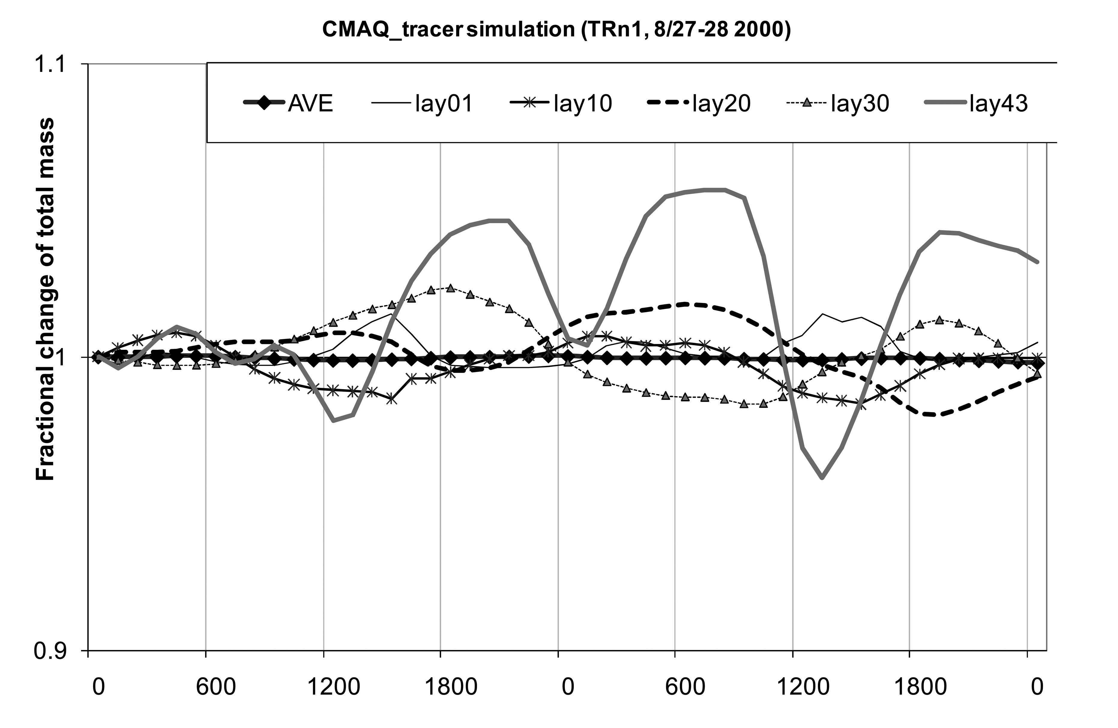
In an operational setting, both run time memory and model speed are strong constraints. One way to reduce both burdens is to reduce the vertical layers of the AQ model. The AQ model often is designed to have a lower model-top and a set of coarsened layers than those of the meteorological model. In the five models considered here, all of them except WRF/Chem practice such layer-collapsing techniques to reduce the overall computational burden. However, reduction of the number of the vertical layers results in a loss of model accuracy. All four of these models attempt to collapse layers where the impact is as minimal as possible and keep one-to-one corresponding layers wherever the atmospheric column typically exhibits strong gradients in meteorological variables, such as gradients in lapse rates, temperature, humidity, wind speed and direction. Even with optimal selection, a reduction in model accuracy invariably occurs. It is the burden of the modeler to assure that the loss of accuracy is minimal and the mass consistency characteristics of the AQ model are not compromised. For the CMAQ model, a recent study by Otte and Pleim [30] has shown that to ensure mass conservation, the resultant thicker layers obtained by collapsing adjacent layers together should not collapse more than two layers for each resultant layer and layer interfaces of the collapsed layers are chosen from the existing interfaces of the original un-collapsed ones. In addition, running the AQ model in tracer mode studies is essential during the engineering design phase to assure preservation of the model's mass consistency characteristics. One important consideration is the time evolution of layer and domain total mass (see Appendix B).
Using a parameter optimization study, Timin et al. [31] proposed that the most important parameters in controlling surface pollutant concentration in AQ models are: (1) h, PBL height; (2) Kz, eddy diffusivity for heat; and (3) Vd, dry deposition velocity of both gaseous and PM species. Lee et al. [32] studied the importance of h, Kz and its parameterization approach on the surface concentration of ozone. Their study reiterated the findings of many other recent investigations [33,34], described in detail later, that the entire diurnal evolution of the PBL, from its nocturnal shallowness to its increase to a maximum late-afternoon depth, are contributing factors to the surface concentrations of airborne pollutants. In Section 2, we will discuss the PBL modeling approaches of the selected five AQ models.
The PBL is intimately related to heat exchange at the air-surface interface. Evaporation is the primary process that governs the partitioning of exchange rates between the sensible and latent portions of the surface energy budget. Therefore, PBL modeling is strongly coupled with land surface modeling (LSM). Since soil moisture and evaporation processes are key parameterizations needed to model surface latent heat fluxes accurately, identifying the uncertainties in modeling these items is important. These are the main questions for LSM. Xiu and Pleim [35] summarized that the primary goal of LSM is to parameterize surface moisture flux.
The same can be said for the strong coupling between dry deposition modeling and LSM, but for mass fluxes. Dry deposition is recognized as an important pathway among the various removal processes for atmospheric trace species. Among many ongoing investigations to understand and quantify this pathway, recent reinforced research efforts in this area by the U.S. Environmental Protection Agency have already shed light on these many related topics [36-38]. Section 3 will discuss the dry deposition velocity modeling of the selected five AQ models.
2. Planetary Boundary Layer
It is the surface fluxes that produce the PBL. As incident sunlight is absorbed by the earth's surface, radiant energy is transformed into sensible and latent heat fluxes from the surface. This heating from the bottom of the atmospheric column produces convective eddies that transport heat and water vapor to warm and moisten air parcels above them. Such a convective eddy also consists of a downward element of heavier and cooler air which accelerates the displacement of the ascending element of buoyant air within the eddy. During the growth phase of the PBL, the ascending eddies penetrate the thermal inversion capping the layer top. They transport heat, moisture and kinetic energy upwards in a counter-gradient manner forming the so-called entrainment zone [39]. The ascending air parcel soon equilibrates itself with the penetrated environment through redistribution of momentum, heat and moisture. In doing so, the air parcel expands the PBL top with its penetration height. This growth phenomenon continues until the PBL height attains its maximum height defined by the height of the capping thermal inversion, and reaches its maximum height at hundreds or even thousands of meters Above Ground Level (AGL) in the late afternoon.
However, the PBL is not always well defined, whenever frontal boundaries, deep convection, or multiple levels thermal inversions are involved [40]. In addition, Dabberdt et al. [40] recommended the establishment of a high-resolution nation-wide observing network to monitor the diurnal variation of PBL heights. Their recommendation stemmed from the conclusion that Air Quality modeling accuracy is significantly limited by the lack of knowledge of the PBL structure and dynamics.
At the approach of sunset, the rapid weakening and eventual loss of incident solar flux at the surface causes a second thermal inversion to form in the bottom of the atmospheric column. This second inversion together with the capping inversion defines the so-called nighttime residual layer, and the second inversion caps the lowest layer to form the stable nocturnal boundary layer [39].
The layers prevailing at night pose different challenges for AQ forecasting. The residual layer may have sustained part of its turbulent mixing mechanically with wind shear. A nocturnal low-level jet may form just above the stable boundary layer as surface friction is de-coupled from the residual layer, giving rise to the potential emergence of a strong horizontal wind. Therefore, the residual layer can behave both as a vertical capped reservoir of pollutants, such as ozone, trapped aloft and as a conduit for the rapid transport of these pollutants to destinations far from their origin [41].
Heterogeneity in Land-Use Land-Cover (LULC) can have strong effects on the PBL both in its development and collapse in the diurnal cycle and in its interactions between the various LULC boundaries in affecting pollutant transport characteristics. For instance, a sea- or lake-breeze can suppress PBL growth. Melas et al. [42] concluded from measurements that under specific conditions a sea-breeze can rapidly decrease the growing maritime PBL height soon after the onset of the breeze.
Banta et al. [43,44] provided valuable insight into the intricate interactions among synoptic flow, land-sea-breeze, and PBL diurnal evolution by studying the air quality data collected in the Houston, TX, area where two consecutive intensive field studies were carried out in August and September of 2000 and 2006, respectively. The latter campaign reinforced and extended what was understood by studies made from the first. The daytime sea-breeze in the Houston-Galveston area often starts with an easterly and southeasterly Galveston Bay breeze around 3:00 pm local time. Then within one to two hours, a larger-scale southerly to southeasterly Gulf of Mexico breeze strengthens and reinforces the easterly, southeasterly flows. The diurnal cycle manifests itself in coastal temperature contrast and produces a steady 24-h rotation of the wind direction about the larger-scale synoptic flow of gradient wind. Banta et al. [43] suggested that if the geotropic gradient wind was light to moderate and was not able to prevail over the bay breeze, a stagnant wind condition would arise just within the coastline around the late afternoon hours resulting in high surface concentration of pollutants. Furthermore, the convergence of these countering flows produces intermittent updrafts that often results in detached pollutant plumes which are transported aloft high above the marine boundary layer and which can be subject to a different wind direction. These pollution plumes strongly affect morning rush hour surface pollutant concentration as the thermal inversions break and eddies entrain the plumes down to the surface. However, Banta et al. [43] also report from measurements that h is not strongly correlated with maximum concentration of surface O3. Other factors, such as the pre-existing stratification condition of the previous night, pose an equally importance influence on the rapid rise of surface O3 concentration in late morning as well as the eventual daily O3 peak concentration [43,44].
Soil moisture governs surface evaporation and thus critically controls the PBL characteristics [35,45]. Deep soil moisture has a large inertia and influences longer-term PBL behaviors. The Pleim and Xiu [46] (hereafter PX) LSM includes soil moisture and soil temperature nudging utilizing a four-dimensional data assimilation (FDDA) scheme using model analysis [46-48]. This scheme yields high quality meteorological fields, especially those within the PBL, to enable longer duration forecasts than those LSMs which have no DA capability such as the U.S. National Centers for Environmental Prediction; Oregon State University; Air Force; Hydrological Research Laboratory (Noah) LSM [49,50]. This resonates with the discussion on prolonging current operational AQ forecast in the previous section.
Table 1 summarizes basic model configurations which directly affect the outcome of PBL parameterization results either due to grid structure alignment between the meteorological model (MET) and the chemical transport model (CTM) or other numerical artifacts. Table 1 states the domain map projection and grid structure, the models' overarching assumptions to their primitive equations; microphysical, radiative parameterization; and removal schemes for air pollutants. In the case of land/sea breezes, the thermally driven processes such as the microphysical and radiative processes are likely to be the major drivers. Table 2 continues Table 1 but focusing on turbulent mixing parameterizations within the PBL itself. The choice of schemes and their interplay with other important physical processes are listed for further discussion. Chemical mechanisms and parameterizations that are deemed to have a less direct affect on the PBL scheme outcomes on turbulent mixing of pollutants are not listed here. A thorough listing of such items for the five selected models are available elsewhere: ECMWF-CHIMERE [1,51]; GATOR-GCMOM [17]; GEM-MACH15 [52,53]; WRF/Chem [7]; and WRF-NMM/CMAQ [54,32]. In grid structures, the inter-leaving, “layer-collapsing” practices of ECMWF-CHIMERE, GATOR-GCMOM, GEM-MACH15 and WRF-NMM/CMAQ introduce potential inaccuracies in coupling between the MET and CTM, especially in upper tropo-spheric layers where the jump in inter-leaving selection of layers in MET is the largest. Appendix B presents a study by Ngan [55] where it was shown that the CTM (in this case, CMAQ) layers preserve the domain total mass over time but layer-specific total mass fluctuates temporally.
The truncated model top for ECMWF-CHIMERE, GATOR-GCMOM, GEM-MACH15 and WRF-NMM/CMAQ also incurs some loss of accuracy. Especially for ECMWF-CHIMERE, the model top of CHIMERE is rather low—topped around 3 km AGL.
The lowest mid-layer thicknesses of the five selected models are comparable. They are obviously too high for direct comparison with AQ monitors which are often situated at about 2–10 m Above Ground Level (AGL). Byun and Dennis [56] showed that model mid-layer values should be extrapolated to monitor levels for matched verification.
All five selected models except WRF-NMM/CMAQ use the classic Mellor and Yamada second order level 2.5 closure model to parameterize the turbulent mixing in PBL. Mellor and Yamada [59] used a local closure scheme to calculate turbulence fluxes. WRF-NMM/CMAQ uses Asymmetric Convective Model (ACM) 2 [62], a combined non-local closure and local gradient diffusion scheme to model mixing processes in the PBL. ACM2 is built on the original ACM non-local convective mixing scheme [64]. The extended scheme now includes an eddy diffusion component. A stability regime specific weighting factor governs the partition of mixing between a nonlocal and local diffusion scheme. For instance, for stable and neutral stabilities, all diffusion is attributed to the local diffusion scheme.
In all the turbulent mixing schemes listed in Table 2, considerable parameterization uncertainties warrant methodological procedures to fine tune the various coefficients and empirical constants employed in the schemes. Among these efforts, Nielsen-Gammon et al. [58] performed a rather vigorous parameter optimization study of the new local convection scheme of ACM2 [62]. Equation 1 states the PBL scaling form of Kz, the vertical eddy diffusivity for heat, within the layer.
Deep soil moisture and temperature govern the slowly varying evaporative component of the soil surface. In all five models, multiple layer soil models are used to calculate heat diffusion and moisture transport of heat and moisture profiles in the top soil stratum. The large inertia of these two quantities makes them attractive variables to be assimilated by observational data. Pleim and Xiu [46] followed the Interactions between Soil, Biosphere, and Atmosphere (ISBA) model [65] to develop an indirect soil moisture nudging algorithm. The scheme uses model biases of the 2 m air temperature to nudge soil moisture. More recently, Pleim and Gilliam [47] added a new technique using biases of the 2 m air temperature to nudge deep soil temperature only during nighttime.
3. Dry Deposition Velocity
Dry deposition velocities of gaseous species and sedimentation velocities of particulate species are sensitive parameters that influence surface concentrations of atmospheric constituents. Table 3 presents the parameterization schemes used by the five models in this study.
Parameter optimization is critical for the applicability of the dry deposition schemes to capture the characteristics of the resistances that are keys in the Wesely and Hicks [68] electrical analog model. The analog is applied to the three resistances in a series circuit, namely: Ra, aerodynamic resistance; Rb, laminar sub-layer resistance; and Rc, canopy resistance. There are large uncertainties in quantifying these resistances, especially Rc where stomatal, and highly variable leaf and twig coverage conditions of the soil surface are subject to parameter optimization. The research work on sub-modeling of these resistances by Erisman et al. [69]; Baer and Nester [72]; Sander [73] and Hall et al. [74] has increased the usefulness of the analog model.
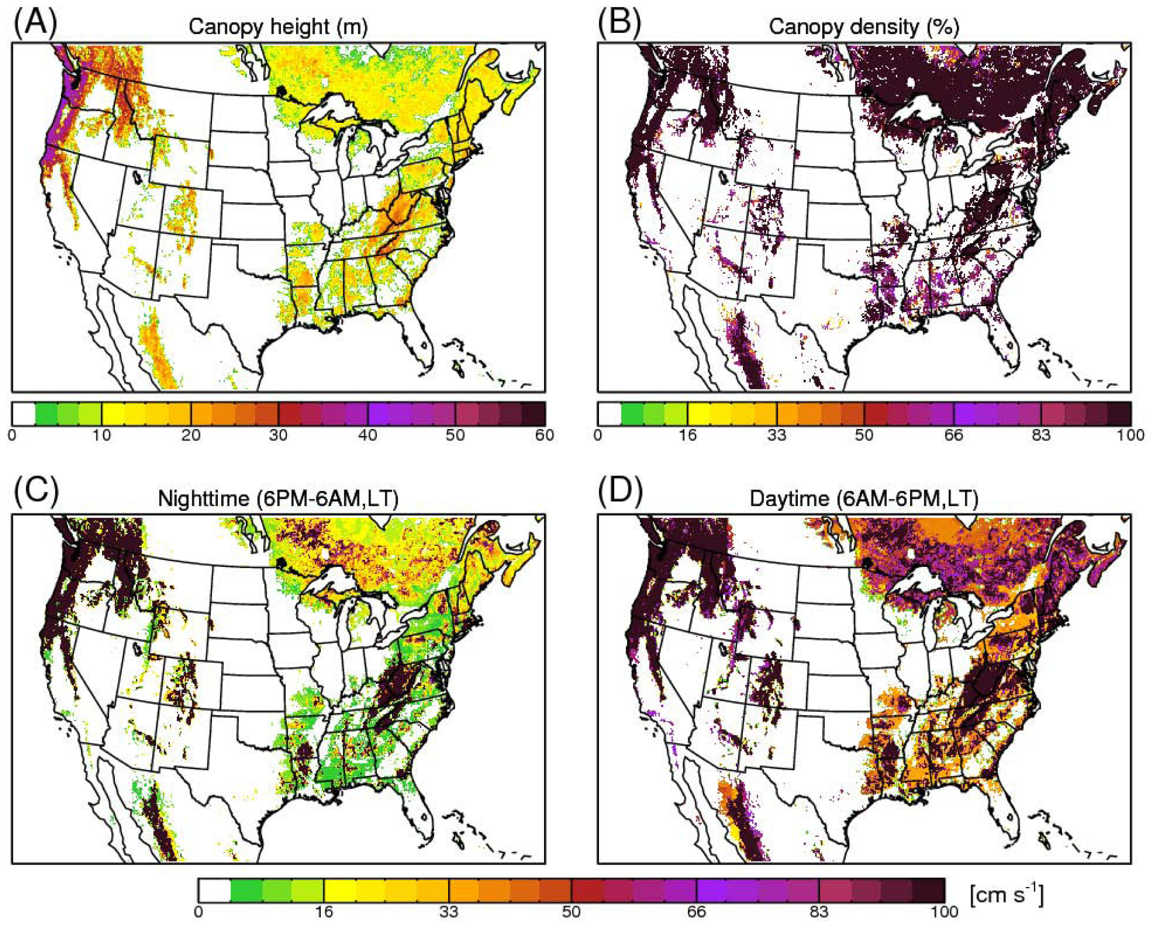
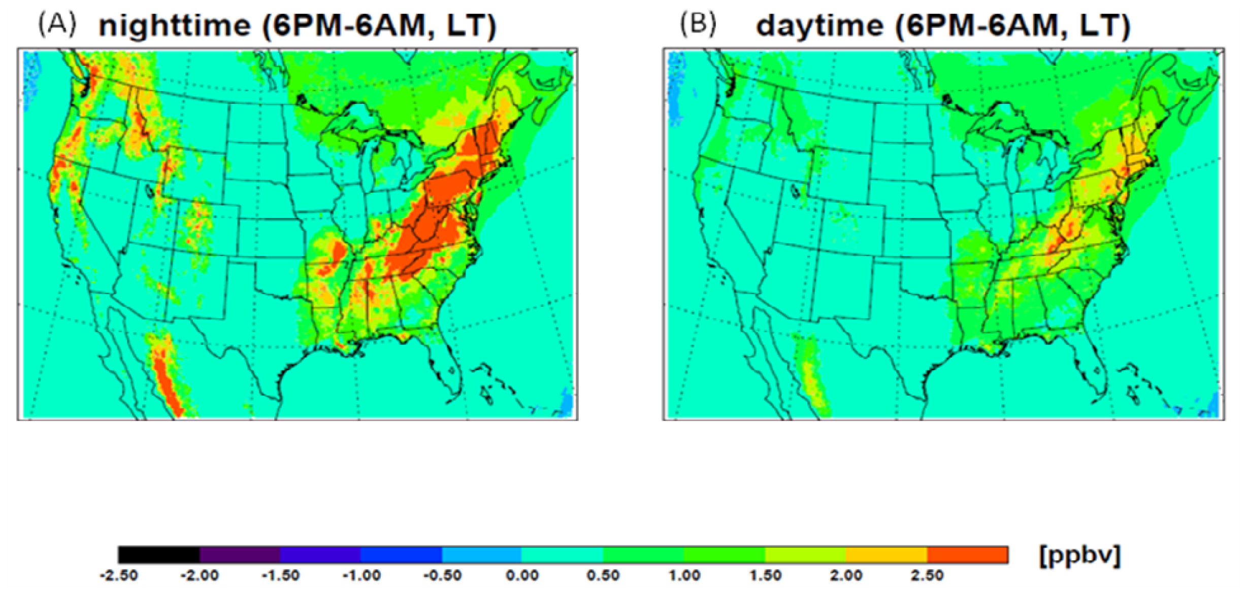
Choi et al. [75] addressed the uncertainty of roughness length used in CTMs. In their study an upper bound value for zo was set to the canopy height in Xiu and Pleim [35] formulation for Ra, as follows:
4. Summary
Physical processes within the PBL contribute important factors governing the characteristics of the diurnally varying surface concentration of the major air pollutant components; such as ozone and particulate matter. Air Quality models that are capable of resolving meso-scale features yet efficient enough to simulate large areas; e.g., continental scale or larger, are the focus of scrutiny in this review. Five models were selected to reveal the various challenges of meeting the accuracy and timeliness of these models in a real-time operational setting.
They are: (a) The European Center for Medium range Weather Forecast meteorology model (ECMWF) coupled with CHIMERE; (b) The Stanford Gas-Aerosol-TranspOrt-Radiation chemistry model (GATOR)—coupled with the General-Circulation-Mesoscale-and-Ocean-Model (GCMOM); (c)The Canadian Global Environmental Multi-scale meteorology model (GEM) coupled with the Modelling Air quality and CHemistry in 15 km horizontal grid resolution (MACH15); (d) The Weather Research and Forecasting (WRF)—Advanced Research WRF (ARW) dynamic core meteorology model coupled with Chemistry (Chem) model; and (e) the WRF—Non-hydrostatic Meso-scale Model (NMM) dynamic core meteorology model coupled with the Community Multi-scale Air Quality model (CMAQ). Among them (a) and (e) adopted offline coupling between its meteorological and chemical transport models; whereas (b), (c), and (d) adopted various degrees of inline coupling. (d) is probably the closest to fully inline coupled, as horizontal and vertical grid structures as well as dynamics and physical packages for the meteorological and chemical transport models are identical and the two-way feedbacks between them are fully functional. Some potential aerosol loading feedbacks have the direct effect of radiation attenuation, and indirect effects, such as increase in concentration in cloud condensation nuclei and precipitation modification.
The focus of this review study is on the two main physical processes within the PBL: turbulent mixing and dry depositions of gaseous and particulate phase constituents among the five models. Three of them used level 2.5 closure models to calculate turbulent mixing within the PBL. The key to model performance in capturing the characteristics of turbulent mixing within the PBL is often attributed to systematic efforts in parameter tuning and optimization of the model or sub-models used. This study quoted a rather thorough parameterization optimization study by Nielsen-Gammon et al. [58] performed for the local convective mixing parameterization scheme within ACM2 [62]. It illustrates the uncertainties involved and the well-invested optimization study utilizing variational methods, which can significantly improve model performance.
This study also revealed that the short-term trend for future AQ model improvement is the emphasis of data assimilation. A case in point is deep soil moisture data assimilation. Literature had repeatedly shown that this large inertia term is critical in understanding its medium- to long-range AQ forecast. The Pleim-Xiu [46] indirect soil moisture nudging algorithm exploits this possibility.
Dry deposition velocity (Vd) parameterization involved an intricate set of sub-modeling, such as: stomatal and land-surface conditions. Therefore, parameter optimization to generate universally applicable parameters for Vd models is the key to versatility and accuracy. This reinforces the importance of uncertainty quantification and parameter optimization mentioned for the model performance for turbulent mixing parameterization schemes.


| MET | ECMWF | a GCMOM | GEM | WRF-ARW | WRF-NMM |
|---|---|---|---|---|---|
| CTM | CHIMERE | b GATOR | MACH15 | Chem | CMAQ |
| CTM/MET Horizontal grid | lat-long/Gaussian | Oblique sterographic | Polar-stereo-graphic/Gaussian | Lambert con-formal conic (lcc) | lcc/Rotated lat-long |
| Resolution (km) | 0.5° | Innermost 5 | 15 | 27 | 12 |
| Vertical grid | Pressure and terrain-following hybrid | σ-z | Pressure and terrain following hybrid c | σ-p | Pressure and terrain following hybrid d |
| Total CTM/MET layers | Lowest 20/91 | Inter-leaved (IL) 26/39 | IL 58/80 | 40/40 | IL 22/60 |
| Model top CTM/MET | ∼3 km/0.01 hPa | 103.5 hPa/0.425 hPa | 0.1 hPa/0.1 hPa | 50 hPa/50 hPa | 100 hPa/0.2 hPa |
| Lowest mid-layer (m) | 15 | 15 | 15 | 16 | 19 |
| Hydrostatic assumption | No | Yes | No | No | No |
| Primitive Equation for CTM | flux | Flux | flux | flux | flux |
| Online coupled | No. | Yes e. Unified. | Yes. Unified. | Yes. Unified. | No. |
| Δt for Data-exchange | 3 h | 5 min | 7 min | 5 min | 1 h |
| Hydrometeors considered | 6: water vapor, water, ice, rain, snow and graupel | Sized resolved droplet & ice crystals | 6: Same as 2nd column of this row | 6: same as column to the left | 6: same as column to the left |
| pm size model (bins) | Sectional (8) | Sectional (17–30) | Sectional (2) | modal | modal |
| Cloud-induced radiative attenuation | Yes | Yes | Yes | Yes | j ratio of S.W.radiative fluxes |
| k In-cloud scavenging | Yes | Yes | Yes | Yes | Yes |
| l Below-cloud scavenging | Yes | Yes.m Detailed coagulation. | Yes | Yes | Yes |
aGCMOM-bGATOR [3].cPure isobaric at top levels and terrain-following in lower levels [6].dWRF/NMM adopts a mixed hybrid ordinate. Its coupling to CMAQ is explained further in Appendix A.eZhang [23] suggested the differentiation of the two types of online coupling that are commonly used. Although both types conduct data exchange per advection time step, (a) the separate coupled type has different physics parameterization schemes between CTM and MET, whereas the unified coupled type shares the same schemes between them.jRatio of short wave solar radiation reaching surface to that under clear sky condition.kIn-cloud scavenging can strictly mean the rain-out process due to uptake of aerosols. However in the context of this table it also refers to the following relevant in-cloud processes leading to the removal of aerosol particles: aerosol activation, nucleation, auto-conversion of cloud droplets, and Brownian diffusion for activated particles.lBelow-cloud scavenging refers to aerosol-hydrometeor coagulation and collection.mWashout occurs upon interactions of each aerosol size with each precipitation droplet size to account for differential fall speeds of the droplets.
| MET | ECMWF | GCMOM | GEM | WRF-ARW | WRF-NMM |
|---|---|---|---|---|---|
| CTM | CHIMERE | GATOR | MACH15 | Chem | CMAQ |
| Turbulence scheme & l LSM pair | Kz & m TESSEL | n Mellor Yamada 2.5 & [57] | Mellor Yamada 2.5 & o PX | p YSU & q Noah | r ACM2 & Noah |
| Theory used for turbulent mixing | Kz s vertical profile | Mellor Yamada 2.5 | Mellor Yamada 2.5 | Mellor Yamada 2.5 | t ACM2 |
| Modification applied | Empirical cut-off t Ri | None | Solved by u Laasonen | None | None |
| Parameter optimization using operational research methodology | None | None | None | None | [58] |
| Surface layer scheme | None | v M-O | M-O | M-O | M-O |
| Possibility w D.A. for soil property nudging | No | No | Yes | No | No |
lLand Surface Model;mTiled ECMWF Scheme for Surface Exchange over Land;nMellor and Yamada [59];oPleim-Xue LSM [35];pYun Sei University PBL non-local mixing scheme [60];qNoah LSM [61];pMellor-Yamada-Janjic turbulent mixing scheme;rAsymmetric Convective Mixing scheme [62];s[63];tCritical bulk Richardson number reaches 0.15 as cutoff for top of PBL [1];uSolved by using a Laasonen implicit differencing scheme;vMonin-Obukhov suface layer scheme;wData Assimilation.
| MET | ECMWF | GCMOM | GEM | WRF-ARW | WRF-NMM |
|---|---|---|---|---|---|
| CTM | CHIMERE | GATOR | MACH15 | Chem | CMAQ |
| Theory applied to gaseous phase | A Electrical analog | Electrical analog | Electrical analog | Electrical analog | Electrical analog |
| Modifications/data upgrade | none | none | B [66] | none | C Scaled canopy height |
| Theory applied to aerosol phase | D Settling velocity modulated by surface resistances | Size resolved sedimentation velocity | E [67] | F Settling velocity of poly-dispersed aerosol | G Settling velocity modulated by aerodynamic and laminar resistance |
A[68];BZhang et al. [66] applied electrical circuit analog model to parameterize dry deposition velocities for 31 gaseous species;CRoughness length is estimated by satellite observed canopy height (see Equation 2 and discussion in this section);D[69];EZhang et al. [67] improved the Canadian Aerosol Module, a predecessor of the current module in GEM-MACH15, with a size sectional approach accounting for turbulent transfer, Brownian diffusion, impaction, interception, gravitational settling, growth in moist environment, and particle rebound;F[70];G[71].
Acknowledgments
We would like to dedicate this paper to Daewon Byun, who was a group lead of NOAA Air Resources Laboratory Air Quality group and passed away in February 2011. We thank all members of the satellite MODIS, and GLAS team members for providing helpful comments on in situ measurements and satellite data reference in this study. The authors also express gratitude to the anonymous reviewers from ARL/NOAA and Atmosphere for their valuable inputs and fine-polishing of this article.
Appendix A
WRF-NMM/CMAQ adopts a hybrid pure pressure upper stratum and a lower mixed stratum contributed by both a pressure-part and a terrain-following-part. There, by definition the hydrostatic pressure for the moist atmosphere is given as
Each model vertical layer thickness can be computed from
Layer thickness
By expressing the layers' pressures in xˆ3, a monotonically increasing generalized co-ordinate, xˆ3 [10], one can compute Jxˆ3, vertical Jacobian, as follows:
Therefore, the Jacobian at the middle of the layer,
Similarly, the Jacobian at the layer interface must be computed utilizing incremental changes of η2 and η1 with respect to the changes in xˆ3.
Note that ρJxˆ3 is not constant with respect to the vertical coordinate due to the changes in the η2 and η1 profiles. However, the fractional contributions of Pd and Pdtop determining ρJxˆ3 does not change with time.
Appendix B
Ngan [55] used the Fifth-Generation NCAR / Penn State Mesoscale Model (MM5) offline coupled with CMAQ4.3 to study O3 episodes in Houston, TX, between 00Z August 27 and 00Z 29, 2000. MM5 meteorological data was fed to CMAQ each simulation hour. MM5 was configured in 43 σ-p vertical layers with variable spacing with the model top set at 50 hPa. CMAQ was configured to run in tracer mode with Trn1, a single species, initially assigned to a constant concentration of unity throughout the entire domain, and subjecting it to lateral boundary condition of unity throughout all levels and sides. Layer-total mass should gain (lose) in accordance with converging (diverging) flows. The domain total mass should be conserved. Figure 1A shows such a total-mass time series illustration for the case studied [55].
References
- Schmidt, H.; Derognat, C.; Vautard, R.; Beekmann, M. A comparison of simulated and observed ozone mixing ratios for the summer of 1998 in western Europe. Atmos. Environ. 2001, 35, 6277–6297. [Google Scholar]
- De Meij, A.; Gzella, A.; Thunis, P.; Cuvelier, C.; Bessagnet, B.; Vinuesa, J.F.; Menut, L. The impact of MM5 and WRF meteorology over complex terrain on CHIMERE model calculations. Atmos. Chem. Phys. Discuss. 2009, 9, 2319–2380. [Google Scholar]
- Jacobson, M.Z. GATOR-GCMM: A global-through urban-scale air pollution and weather forecast model 1. Model design and treatment of subgrid soil, vegetation, roads, rooftops, water, sea, ice, and snow. J. Geophys. Res. 2001, 106, 5385–5401. [Google Scholar]
- Jacobson, M.Z. GATOR-GCMM: 2. A study of day- and nighttime ozone layers aloft, ozone in national parks, and weather during the SARMAP Field Campaign. J. Geophys. Res. 2001, 106, 5403–5420. [Google Scholar]
- Jacobson, M.Z. History of, Processes in, and Numerical Techniques in GATOR-GCMOM. 2010. Available online: http://www.stanford.edu/group/efmh/GATOR/index.html (accessed on 27 June 2011). [Google Scholar]
- Talbot, D.; Moran, M.D.; Bouchet, V.; Crevier, L.-P.; Menard, S.; Kallaur, A. Development of a New Canadian Operational Air Quality Forecast Model. In Air Pollution Modeling and Its Application XIX; Borrego, C., Miranda, A.I., Eds.; Springer: Berlin, Germany, 2009; pp. 470–478. [Google Scholar]
- Grell, G.A.; Peckham, S.E.; Schmitz, R.; McKeen, S.A.; Frost, G.; Skamarock, W.C.; Eder, B. Fully coupled “online” chemistry within the WRF model. Atmos. Environ. 2005, 39, 6957–6975. [Google Scholar]
- Grell, G.A.; Fast, J.; Gustafson, W.I.; Peckham, S.E.; McKeen, S.A.; Salzmann, M.; Freitas, S. On-Line Chemistry within WRF: Description and Evaluation of a State-of-the-Art Multiscale Air Quality and Weather Prediction Model Integrated Systems of Meso-Meteorological and Chemical Transport Models, 1st ed.; Springer: Berlin, Germany, 2011; Chapter 3; pp. 41–54. [Google Scholar]
- Janjic, Z.I. A nonhydrostatic model based on a new approach. Meteorol. Atmos. Phys. 2003, 82, 271–285. [Google Scholar]
- Byun, D.; Schere, K.L. Review of the governing equations, computational algorithms, and other components of the Models-3 Community Multi-scale Air Quality (CMAQ) modeling system. Appl. Mech. Rev. 2006, 59, 51–77. [Google Scholar]
- Foley, K.M.; Roselle, S.J.; Appel, K.W.; Bhave, P.V.; Pleim, J.E.; Otte, T.L.; Mathur, R.; Sarwar, G.; Young, J.O.; Gilliam, R.C.; et al. Incremental testing of the Community Multiscale Air Quality (CMAQ) modeling system version 4.7. Geosci. Model Dev. 2010, 3, 205–226. [Google Scholar]
- Jacobson, M.Z.; Lu, R.; Turco, P.R.; Toon, O.B. Development and application of a new air pollution model system, I, Gas-phase simulations. Atmos. Environ. 1996, 30B, 1939–1963. [Google Scholar]
- Jacobson, M.Z. Development of mixed-phase clouds from multiple aerosol size distributions and the effect of the clouds on aerosol removal. J. Geophys. Res. 2003, 108, 4245. [Google Scholar] [CrossRef]
- Jacobson, M.Z. A solution to the problem of nonequilibrium acid/base gas-particle transfer at long time step. Aerosol Sci. Technol. 2005, 39, 92–103. [Google Scholar]
- Jacobson, M.Z. Effects of absorption by soot inclusions within clouds and precipitation on global climate. J. Phys. Chem. 2006, 110, 6860–6873. [Google Scholar]
- Jacobson, M.Z.; Wilkerson, J.T.; Naiman, A.D.; Lele, S.K. The effects of aircraft on climate and pollution. Part I: A model that treats the subgrid evolution of discrete size- and compostion-resolved contrails from all commercial flights worldwide. J. Geophys. Res. 2007, 112, D11307. [Google Scholar] [CrossRef]
- Jacobson, M.Z.; Kaufmann, Y.J.; Rudich, Y. Examining feedbacks of aerosols to urban climate with a model that treats 3-D clouds with aerosol inclusions. J. Geophys. Res. 2007, 112, D24205. [Google Scholar] [CrossRef]
- Gal-Chen, T.; Somerville, R.C. On the use of coordinate transformation for the solution of Navier-Stokes equations. J. Comput. Phys. 1975, 17, 209–218. [Google Scholar]
- Grell, G.A.; Emeis, S.; Stockwell, W.R.; Schoenemeyer, T.; Forkel, R.; Michalakes, J.; Knoche, R.; Seidl, W. Application of a multiscale, coupled MM5/chemistry model to the complex terrain of the VOTALP valley campaign. Atmos. Environ. 2000, 34, 1435–1453. [Google Scholar]
- Peckham, S.E. Evaluation of WRF-Chemistry air quality forecasts produced during CalNex-2010. Preprints. Proceedings of the 91st American Meteorological Society Annual Meeting, Seattle, WA, USA, 24–28 January 2011.
- Fast, J.D.; Gustafson, W.I.; Easter, R.C.; Zaveri, R.A.; Barnard, J.C.; Chapman, E.G.; Grell, G.A.; Peckham, S.E. Evolution of ozone, particulates, and aerosol direct radiative forcing in the vicinity of Houston using a fully coupled meteorology-chemistry-aerosol model. J. Geophys. Res. 2006, 111, D21305. [Google Scholar] [CrossRef]
- Kaiser, J.W.; Benedetti, A.; Flemming, J.; Morcrette, J.-J.; Heil, A.; Schultz, M.G.; van der Werf, G.R.; Wooster, M.J. From Fire Observations to Smoke Plume Forecasting in the MACC Services. Proceedings of the Earth Observation for Land-Atmosphere Interaction Science, Frascati, Italy, 3-6 November 2010.
- Zhang, Y. Online-coupled meteorology and chemistry models: History, current status, and outlook. Atmos. Chem. Phys. 2008, 8, 2895–2932. [Google Scholar]
- Schmale, J.; Schneider, J.; Ancellet, G.; Quennehen, B.; Stohl, A.; Sodemann, H.; Burkhart, J.; Hamburger, T.; Arnold, S.R.; Schwarzenboeck, A.; et al. Source identification and airborne chemical characterisation of aerosol pollution from long-range transport over Greenland during POLARCAT summer campaign 2008. Atmos. Chem. Phys. Discuss. 2011, 11, 7593–7658. [Google Scholar]
- Nolte, C.G.; Gilliland, A.B.; Hogrefe, C.; Mickley, L.J. Linking global to regional models to assess future climate impacts on surface ozone levels in the United States. J. Geophys. Res. 2008, 113, D14307. [Google Scholar] [CrossRef]
- Huang, J.; Minnis, P.; Chen, B.; Huang, Z.; Liu, Z.; Zhao, Q.; Yi, Y.; Ayers, J.K. Long-range transport and vertical structure of Asian dust from CALIPSO and surface measurements during PACDEX. J. Geophys. Res. 2008, 113, D23212. [Google Scholar] [CrossRef]
- Wang, J.X.L.; Gaffen, D.J. Late-twentieth-century climatology and trends of surface humidity and temperature in China. J. Clim. 2001, 2001, 2833–2845. [Google Scholar]
- Bechtold, P.; Kohler, M.; Jung, T.; Doblas-Reyes, F.; Leutbecher, M.; Rodwell, M.J.; Vitart, F.; Balsamo, G. Advances in simulating atmospheric variability with the ECMWF model: From synoptic to decadal time-scales. Q. J. R. Meteorol. Soc. 2008, 134, 1337–1351. [Google Scholar]
- Benjamin, S.G.; Devenyi, D.; Weygandt, S.S.; Brundage, K.J.; Brown, J.M.; Grell, G.A.; Kim, D.; Schwartz, B.E.; Smirnova, T.G.; Smith, T.L.; et al. An hourly assimilation/forecast cycle: The RUC. Mon. Weather Rev. 2004, 132, 495–518. [Google Scholar]
- Otte, T.L.; Pleim, J.E. The meteorology-chemistry interface processor (MCIP) for the CMAQ modeling system: Updates through MCIPv3.4.1. Geosci. Model Dev. 2010, 3, 243–256. [Google Scholar]
- Timin, B.; Wesson, K.; Dolwick, P.; Possiel, N.; Phillips, S. An exploration of model concentration differences between CMAQ and CAMx, Preprints. Proceedings of the 6th Annual CMAS Conference, Chapel Hill, NC, USA, 1–3 October 2007; Available online: http://www.cmascenter.org/conference/2007/agenda.cfm (accessed on 29 June 2011).
- Lee, P.; Tang, Y.; Kang, D.; McQueen, J.; Tsidulko, M.; Huang, H.C.; Lu, S.; Hart, M.; Lin, H.M.; Yu, S. Impact of consistent boundary layer mixing approaches between NAM and CMAQ. Environ. Fluid Mech. 2009, 9, 23–42. [Google Scholar]
- Han, Z.; Zhang, M.; An, J. Sensitivity of air quality model prediction to parameterization of vertical eddy diffusivity. Environ. Fluid Mech. 2009, 9, 73–89. [Google Scholar]
- Lee, S.M.; Giori, W.; Princevac, M.; Fernando, H.J.S. Implementation of a stable PBL Turbulence parameterization for the mesoscale model MM5: Nocturnal flow in complex terrain. Bound. Layer Meteorol. 2006, 119, 109–134. [Google Scholar]
- Xiu, A.; Pleim, J.E. Development of a land surface model. Part I: Application in a mesoscale meteorological model. J. Appl. Meteorol. 2001, 40, 192–209. [Google Scholar]
- Bash, J.O.; Walker, J.T.; Katul, G.G.; Jones, M.R.; Nemitz, E.; Robarge, W. Estimation of in-canopy ammonia sources and sinks in a fertilized Zea Mays field. Environ. Sci. Technol. 2010, 44, 1683–1689. [Google Scholar]
- Wu, Y.H.; Brashers, B.; Finkelstein, P.L.; Pleim, J.E. A multilayer biochemical dry deposition model. 1. Model formulation. J. Geophys. Res. Atmos 2003, 108, 4013. [Google Scholar] [CrossRef]
- Wu, Y.H.; Brashers, B.; Finkelstein, P.L.; Pleim, J.E. A multilayer biochemical dry deposition model. 2. Model evaluation. J. Geophys. Res. Atmos 108.
- Stull, R.B. An Introduction to Boundary Layer Meteorology; Springer: Berlin, Germany, 1988. [Google Scholar]
- Dabberdt, W.F.; Hales, J.; Zubrick, S.; Crook, A.; Krajewski, W.; Doran, J.C.; Mueller, C.; King, C.; Keener, R.N.; Bornstein, R.; et al. Forecast Issues in the Urban Zone: Report of the 10th Prospectus development team of the U.S. weather research program. Bull. Am. Meteorol. Soc. 2000, 81, 2047–2064. [Google Scholar]
- Yerramilli, A.; Challa, V.S.; Dodla, V.B.R.; Dasari, H.P.; Young, J.H.; Patrick, C.; Baham, J.M.; Huges, R.L.; Hardy, M.G.; Swanier, S.J. Simulation of surface ozone pollution in the Central Gulf coast region using WRF/Chem model: Sensitivity to PBL and land surface physics. Adv. Meteorol. 2010, 2010, 319138. [Google Scholar] [CrossRef]
- Melas, D.; Abbate, G.; Haralampopoulos, D.; Kelesidis, A. Estimation of meteorological parameters for air quality management: Coupling sodar data with simple numerical models. J. Appl. Meteorol. 2000, 39, 509–515. [Google Scholar]
- Banta, R.M.; Senff, C.J.; Nielsen-Gammon, J.; Darby, L.S.; Ryerson, T.B.; Alvarez, R.J.; Sandberg, S.P.; Williams, E.J.; Trainer, M.K. A bad air day in Houston. Bull. Am. Meteorol. Soc. 2005, 86, 657–669. [Google Scholar] [CrossRef]
- Banta, R.M.; Senff, C.J.; Alvarez, R.J.; Langford, A.O.; Parrish, D.D.; Trainer, M.K.; Darby, L.S.; Hardesty, R.M.; Lambeth, B.; Neuman, J.A.; et al. Dependence of daily peak O3 concentrations near Houston, Texas on environmental factors: Wind speed, temperature, and boundary-layer depth. Atmos. Environ. 2011, 45, 162–173. [Google Scholar]
- Zhang, D.-L.; Anthes, R.A. A high-resolution model of the planetary boundary layer—Sensitivity tests and comparisons with SESAME-79 data. J. Appl. Meteorol. 1982, 21, 1594–1609. [Google Scholar]
- Pleim, J.E.; Xiu, A. Development of a land surface model. Part II: Data assimilation. J. Appl. Meteorol. 2003, 42, 1811–1821. [Google Scholar]
- Pleim, J.E.; Gilliam, R. An indirect data assimilation scheme for deep soil temperature in the Pleim-Xiu land surface model. J. Appl. Meteorol. 2009, 48, 1362–1375. [Google Scholar]
- Gilliam, R.; Pleim, J. Performance assessment of new land surface and planetary boundary layer physics in the WRF-ARW. J. Appl. Meteorol. 2010, 49, 760–774. [Google Scholar]
- Pan, H.L.; Mahrt, L. Interaction between soil hydrology and boundary-layer development. Bound. Layer Meteor 1987, 38, 185–202. [Google Scholar]
- Chen, F.; Mitchell, K.; Schaake, J.; Xue, Y.; Pan, H.L.; Koren, V.; Duan, Q.Y.; Ek, M.; Betts, A. Modeling of land surface evaporation by four schemes and comparison with FIFE observations. J. Geophys. Res. 1996, 101, 7251–7268. [Google Scholar]
- Heil, A.; Kaiser, J.W.; van der Werf, G.R.; Wooster, M.J.; Schultz, M.G.; van der Gon, D.H. Assessment of the real-time fire emissions (gfasv0) by macc, ECMWF Tech.; Memo No. 628; ECMWF: Reading, UK, 2010. [Google Scholar]
- Smyth, S.C.; Jiang, W.; Roth, H.; Moran, M.; Makar, P.; Yang, F.; Bouchet, V.; Landry, H. A comparative performance evalutation of the AURAMS and CMAQ air-quality modeling system. Atmos. Environ. 2009, 43, 1059–1070. [Google Scholar]
- Makar, P.; Moran, M.; Menard, S.; Gong, S.; Gong, W.; Huang, P.; Stroud, G.; Kallaur, A.; Landry, H.; Anselmo, D.; et al. Algorithms for GEM-MACH15: Constructing Canada's new operational air-quality forecast model. Proceedings of the 1st annual International Aerosol Modeling Algorithms (IAMA) Conference, Davis, CA, USA, 7-11 December 2009; pp. 1–35.
- Eder, B.; Kang, D.; Mathur, R.; Pleim, J.; Yu, S.; Otte, T.; Pouliot, G. A performance evaluation of the national air quality forecast capability for the summer of 2007. Atmos. Environ. 2009, 43, 2312–2320. [Google Scholar]
- Ngan, F. Classification of weather patterns and improvement of meteorological inputs for TexAQS-II air quality simulations. Ph.D. Thesis, Department of Geosciences, University of Houston, TX, USA, 2008. [Google Scholar]
- Byun, D.W.; Dennis, R. Design artifacts in Eulerian air quality models: Evaluation of the effects of layer thickness and vertical profile correction on surface ozone concentrations. Atmos. Environ. 1995, 29, 105–126. [Google Scholar]
- Rhee, T.S.; Brenninkmeijer, C.A.M.; Rockmann, T. The overwhelming role of soils in the global atmospheric hydrogen cycle. Atmos. Chem. Phys. 2006, 6, 1611–1625. [Google Scholar]
- Nielsen-Gammon, J.W.; Hu, X.M.; Zhang, F.; Pleim, J.E. Evaluation of planetary boundary layer scheme sensitivities for the purpose of parameter estimation. Mon. Weather Rev. 2010, 138, 3400–3417. [Google Scholar]
- Mellor, G.; Yamada, T. Development of a turbulent closure model for geophysical fluid problems. Rev. Geophys. 1982, 20, 851–875. [Google Scholar]
- Hong, S.Y.; Noh, Y.; Dudhia, J. A new vertical diffusion package with an explicit treatment of entrainment processes. Mon. Weather Rev. 2006, 134, 2318–2341. [Google Scholar]
- Ek, M.B.; Mitchell, K.E.; Lin, Y.; Grunmann, P.; Rogers, E.; Gayno, G.; Koren, V. Implementation of the upgraded Noah land-surface model in the NCEP operational meso-scale Eta model. J. Geophys. Res. 2003, 108, 8851. [Google Scholar]
- Pleim, J.E. A combined local and nonlocal closure model for the atmospheric boundary layer. Part I: Model description and testing. J. Appl. Meteorol. Climatol. 2007, 46, 1383–1395. [Google Scholar]
- O'Brien, J.J. A note on the vertical structure of the eddy exchange coefficient in the planetary boundary layer. J. Atmos. Sci. 1970, 27, 1213–1215. [Google Scholar]
- Pleim, J.E.; Chang, J.S. A non-local closure model for vertical mixing in the convective boundary layer. Atmos. Environ. 1992, 26A, 965–981. [Google Scholar]
- Bouttier, F.; Mahfouf, J.F.; Joilhan, J. Sequential assimilation of soil moisture from atmosphere low-level parameterization. Part I: Sensitivity and calibration studies. J. Appl. Meteorol. 1993, 32, 1335–1351. [Google Scholar]
- Zhang, L.; Moran, M.D.; Makar, P.A.; Brook, J.R.; Gong, S.L. Modeling gaseous dry deposition in AURAMS: a unified regional air-quality modeling system. Atmos. Environ. 2002, 36, 537–560. [Google Scholar]
- Zhang, L.; Gong, S.L.; Padro, J.; Barrie, L. A size-segregated particle dry deposition scheme for an atmospheric aerosol module. Atmos. Environ. 2001, 35, 549–560. [Google Scholar]
- Wesley, M.I.; Hicks, B.B. Some factors that affect the deposition rates of sulfur dioxide and similar gases on vegetation. J. Air Pollut. Control Assoc. 1977, 127, 1110–1116. [Google Scholar]
- Erisman, J.W.; van Pul, W.; Wyers, G. Parameterization of surface resistance for the quantification of atmospheric deposition of acidification pollutants and ozone. Atmos. Environ. 1994, 28, 2595–2607. [Google Scholar]
- Pleim, J.E.; Venkatram, A.; Yamartino, R. ADOM/TADAP Model Development Program. In The Dry Deposition Module; Ontario Ministry of the Environment: Toronto, Canada, 1984; Volume 4. [Google Scholar]
- Venkatram, A.; Pleim, J. The electrical analogy does not apply to modeling dry deposition of particles. Atmos. Environ. 1999, 33, 3075–3076. [Google Scholar]
- Baer, M.; Nester, K. Parameterization of trace gas dry deposition velocities for a regional mesoscale diffusion model. Ann. Geophys. 1992, 10, 912–923. [Google Scholar]
- Sander, R. Compilation of Henry's Law Constants for inorganic and organic species of potential importance in environment chemistry; Air Chemistry Department Max-Planck Institute of Chemistry: Mainz, Germany, 1999. [Google Scholar]
- Hall, B.; Claiborn, C.; Baldocchi, D. Measurement and modeling of the dry deposition of peroxides. Atmos. Environ. 1999, 33, 577–589. [Google Scholar]
- Choi, Y.; Byun, D.; Lee, P.; Saylor, R.; Kim, H.; Lefsky, M. The impact of satellite-derived canopy heights on improving ground-level O3 simulation over Eastern U.S. Geophys. Res. Lett. 2011. submitted for publication. [Google Scholar]
- Lefsky, M.A. A global forest canopy height map from the Moderate Resolution Imaging Spectroradiometer and the Geoscience Laser Altimeter System. Geophys. Res. Lett. 2010, 37, L15401. [Google Scholar] [CrossRef]
- Brutsaert, W. Evaporation into the Atmosphere: Theory, History, and Applications; Wilfried, H., Brutsaert, D., Eds.; Reidel Publishing: Dordrecht, Holland, 1982. [Google Scholar]
© 2011 by the authors; licensee MDPI, Basel, Switzerland. This article is an open access article distributed under the terms and conditions of the Creative Commons Attribution license (http://creativecommons.org/licenses/by/3.0/).
Share and Cite
Lee, P.; Ngan, F. Coupling of Important Physical Processes in the Planetary Boundary Layer between Meteorological and Chemistry Models for Regional to Continental Scale Air Quality Forecasting: An Overview. Atmosphere 2011, 2, 464-483. https://doi.org/10.3390/atmos2030464
Lee P, Ngan F. Coupling of Important Physical Processes in the Planetary Boundary Layer between Meteorological and Chemistry Models for Regional to Continental Scale Air Quality Forecasting: An Overview. Atmosphere. 2011; 2(3):464-483. https://doi.org/10.3390/atmos2030464
Chicago/Turabian StyleLee, Pius, and Fong Ngan. 2011. "Coupling of Important Physical Processes in the Planetary Boundary Layer between Meteorological and Chemistry Models for Regional to Continental Scale Air Quality Forecasting: An Overview" Atmosphere 2, no. 3: 464-483. https://doi.org/10.3390/atmos2030464