Cross-Comparison of MODIS and CloudSat Data as a Tool to Validate Local Cloud Cover Masks


Abstract
: This paper presents a cross-comparison of the data acquired by the MODIS and CloudSat sensors in order to understand the limit of the developed cloud-mask algorithm and to provide a quantitative validation assessment of cloud masks by using exclusively remotely sensed data. The analysis has been carried out by comparing both the intermediate levels of the cloud mask such as the brightness temperatures and the reflectance values for different channels, and the cloud mask itself with the cloud profiles as measured by the CloudSat sensor. The comparison between MODIS cloud tests and the CloudSat profiles indicates an agreement with hit rates (H) and Hanssen-Kuiper Skill Score (KSS) varying between 0.7 and 1.0 and 0.4 and 1.0, respectively. In this case, the low values of H and KSS are found due to the limitation of CloudSat to detect low clouds. The comparison between the cloud mask and the CloudSat profile determines H and KSS values between 0.6 and 1, except for one case. The CloudSat profile has also been compared with the Standard MODIS cloud mask in order to understand the improvement obtained in the use of local adapted thresholds. A comparison of MODIS and CALIPSO data is also presented.1. Introduction/Motivation
The detection of cloud is an important issue in many applications. In the Arctic region, cloud presence has a strong impact on the energy budget since it controls sea ice growth and melt [1]. In tropical and/or subtropical areas, the detection of stratocumulus and shallow cumulus clouds is a key issue, especially over oceans that have a strong negative cloud forcing and whose dependence on environmental conditions is important for explaining overall climate sensitivity.
By using remotely sensed data, cloud cover detection is mainly based on visible and infrared window thresholds despite the difficulties they present. In fact, many conditions of the terrestrial surfaces reduce cloud contrast in some spectral regions (e.g., bright clouds over snow and ice). Furthermore, cloud types such as thin cirrus, low-level stratus at night, and small cumulus typically have low contrast with the underlying background. Cloud edges cause further difficulties because the instrument field of view is almost always neither completely obscured by clouds nor completely clear [2].
In order to detect a reliable cloud mask the MODIS Cloud Mask Algorithm, MCMA, [2,3] uses several cloud-detection tests. Based on previous considerations, the accuracy of cloud detection using satellite observations varies with underlying surface types thus further complicating analysis based on cloud detection such as cloud-radiative feedback mechanisms and climate change analysis [1].
Moreover, as MCMA was developed to be applied at a global level, then in many cases the development of a cloud mask that meets local conditions is required [4]. In this context, having a tool to validate and perform a quantitative assessment of the newly developed cloud mask is a key issue in order to evaluate the effectiveness of the adapted tests and the new final cloud mask.
In some cases, the validation is carried out through a visual inspection in order to qualitatively evaluate the effect of the different tests used for the cloud detection [5]. Some terrestrial tools have also been considered for validation purposes, such as airborne flights and lidar systems [2,6].
The recent availability of data from A-train sensors such as CloudSat and CALIPSO (Cloud-Aerosol Lidar and Infrared Pathfinder Satellite Observation) provides, for the first time, near simultaneous measurements of clouds, aerosols, temperature, relative humidity and radiative fluxes over the globe during all seasons [7]. In particular, the cloud profiling radar (CPR) onboard CloudSat can penetrate deeply in nearly all cases of non-precipitating clouds. The main limitation remains the reduced sensitivity to thin cirrus especially due to the small particle sizes [1,8] and to very low clouds (with heights below 1.0–1.2 km) [9]. The CALIPSO cloud-aerosol lidar is, however, highly sensitive to both optically thin and very low clouds. The combination of these two sensors, CALIPSO/MODIS is of utmost importance in improving cloud detection algorithms. Until now, some studies have been dedicated to the comparison of MODIS data with CALIPSO measurements [10] in order to provide direct information and assessment on the single tests for cloud coverage for new methodology development [11].
Among these studies, Liu et al. 2010 [1] use MODIS and CALIPSO data for their different sensitivity to clouds in areas with underlying presence of ice and/or snow and water in Arctic regions. A few studies have been carried out for the comparison of MODIS and CloudSat measurements for validation purposes [12–14].
The main aim of this work is to use CloudSat data as a tool for the validation of local adapted cloud cover masks derived from MODIS images.
This work presents a methodology and the correspondent analysis carried out on some cloud cover tests by using CloudSat data as a validation tool. The comparison of MODIS and CALIPSO data is also presented.
The main objectives of the present work are:
To perform, using CloudSat acquisitions, a quantitative assessment of the cloud detection algorithm based on MODIS images when the MCMA tests have been adapted to meet local conditions;
To develop a methodology to make the comparison between MODIS and CloudSat data feasible.
2. Data
MODIS and CloudSat data have been analyzed for 11 dates from 2006 to 2009 in different seasons. The area of interest is the Mediterranean basin, with a special focus on Southern Italy, where land and sea are interconnected and land ecosystems are quite heterogeneous. It constitutes a very complex environment where the MCMA is often difficult to apply [5].
The MODIS files used for the cloud cover generation are: MOD 021KM (level-1B granule images) and MOD03 (geolocation data sets) data downloaded from [15] and [16].
The corresponding CloudSat and CALIPSO tracks are available from the website [17]. Along with CloudSat and CALIPSO acquisitions, the MODIS-AUX data which correspond to the area detected by these sensors can be downloaded.
The MODIS-AUX tracks are particularly useful in the comparison between the respective cloud profiles because they are perfectly geolocated with CloudSat profiles as the latitude and longitude files are also available. The 2D cloud cover images derived from MOD 021KM are then used for visual inspection of the results.
3. Methods
The main objective of the conjoint processing of MODIS and CloudSat tracks is to use the cloud profiles detected by CloudSat for validation of the tests performed on MODIS data and of the final local adapted cloud mask. The same procedure can also be applied to CALIPSO data.
In order to verify the applicability of the proposed procedure from MODIS cloud mask, the following tests have been selected:
- -
Test 1: Brightness temperature at 11 μm, BT 11;
- -
Test 2: Difference of brightness temperature at 11 and 3.7 μm, BT 11–BT 3.7;
- -
Test 3: Reflectance at 1.38 μm, ρ1.38;
- -
Test 4: Difference of brightness temperature at 3.7 and 12 μm, BT 3.7–BT 12.
The proposed processing can also be used for the other tests.
For each of these tests, an adaption of the thresholds has been performed starting from the original MCMA [2,3]. In fact, these thresholds depend on a considerable number of parameters, such as the time of the acquisition, the latitude, the underlying ecosystem and the atmospheric conditions. Then, starting from the original thresholds they are adapted to local/regional conditions of Southern Italy, resulting in an algorithm based on different tests [4,18]. The found thresholds for this area are listed in Table 1.
Starting from these values, three main classes relating to cloud presence are taken into account [3]:
- -
CCS: confident clear sky. This class corresponds to the probability between 0.99 and 1.0 in the MCMA standard algorithm;
- -
CC: confident cloudy. This class corresponds to the probability between 0 and 0.66 in the MCMA standard algorithm;
- -
INT: intermediate. This class puts together the probability level from 0.66 to 0.95 (probably cloud) and from 0.95 and 0.99 (probably not cloud).
These classes and probability levels are derived from the fact that the thresholds mainly determine two classes: cloudy sky (indicated with probability 0) and not cloudy sky (indicated with probability 1). All the intermediate conditions between these two extreme values are indicated with different levels of probability based on a linear relationship [3,4].
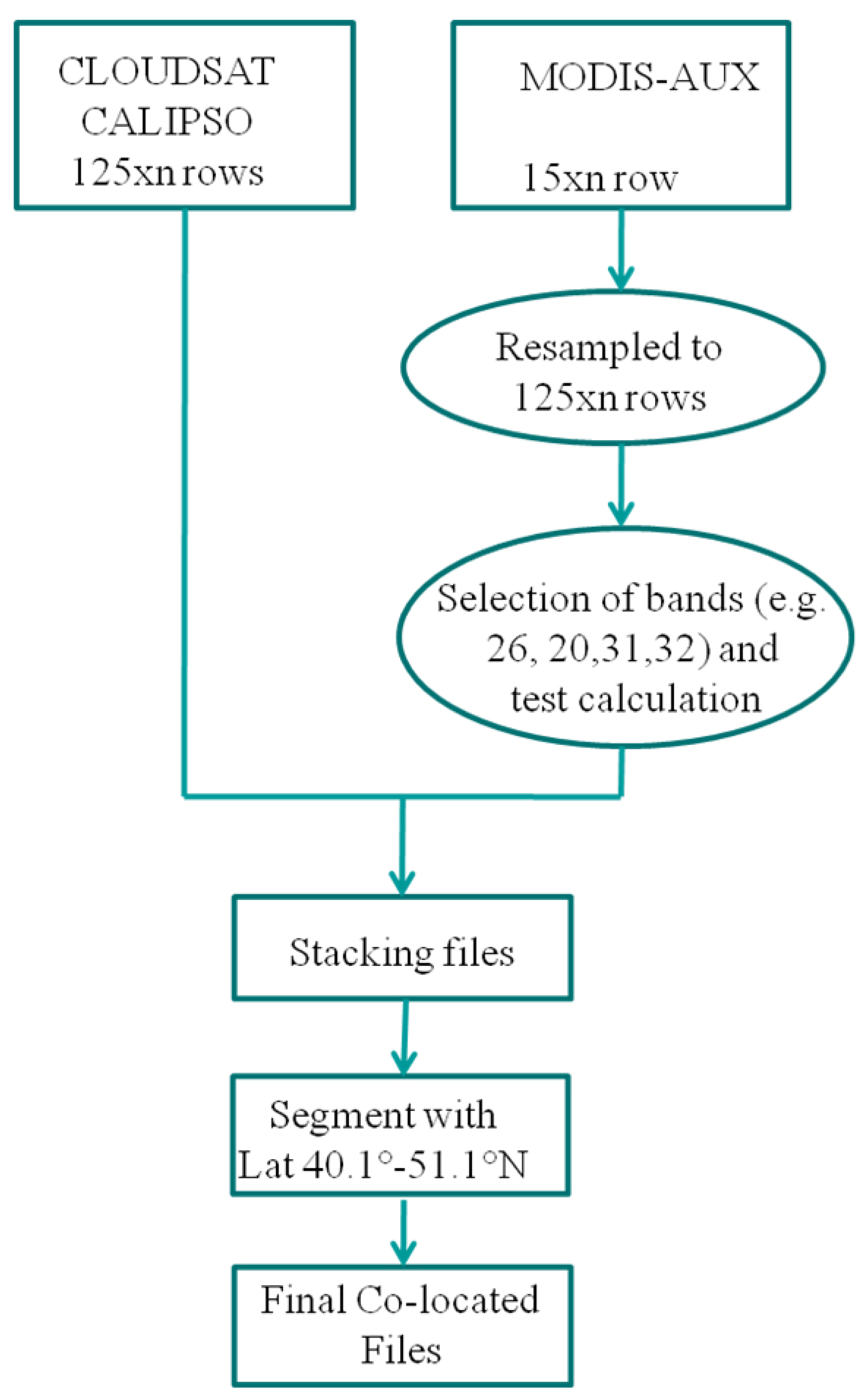
The flowchart in Figure 1 indicates the pre-processing steps necessary in order to have co-located MODIS, CloudSat and CALIPSO data.
After the resampling of the MODIS tracks, the bands useful for cloud detection are extracted and the formulae to obtain the radiance or reflectance values are applied on these bands. Finally, the corresponding variables used for the cloud detection tests are calculated (Table 1). These variables are then stacked together with the information of cloud profile detected by CloudSat and CALIPSO.
In this analysis, two main variables are taken into account:
- -
From file CS_2B-GEOPROF, the cloud scenario is considered. The cloud presence is classified based on the signal received with respect to the background noise by using the SEM (Significant Echo Mask) algorithm. A level of uncertainty is associated with each class. In order to have a one-dimensional profile to be compared with MODIS data, a weighted average has been considered for the classes 6 to 40 [19]. The classes −9 (missing data) and 5 (probable signal from the ground) have not been considered in the averaging.
From file CS_2B-GEOPROF-LIDAR, the cloud fraction and the uncertainties of cloud fraction are considered. The cloud fraction represents the lidar signal in the radar resolution cell (in terms of volume) and ranges from 0 to 100. In order to have a one dimensional profile comparable with MODIS data, a weighted average has been considered for these values. The final values range from 40 (no cloud) to 70 (cloudy) [20].
4. Results and Discussion
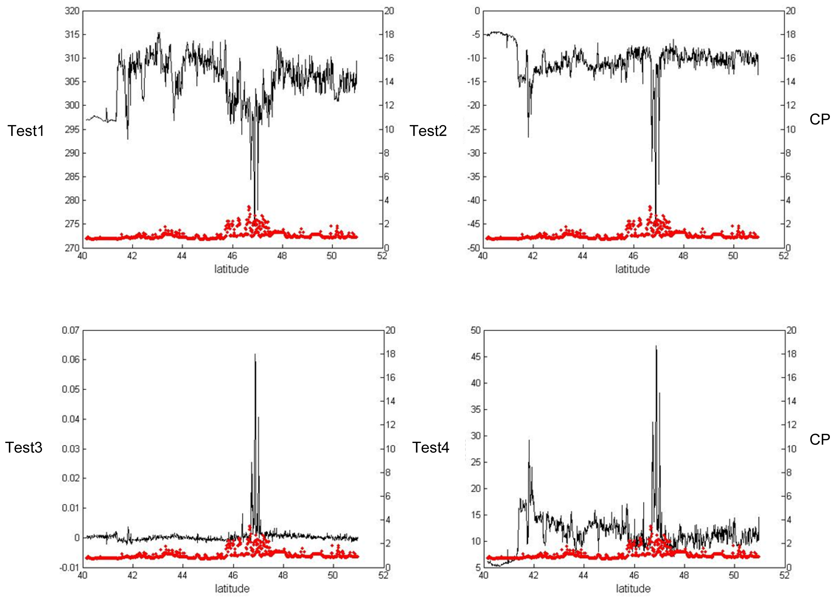
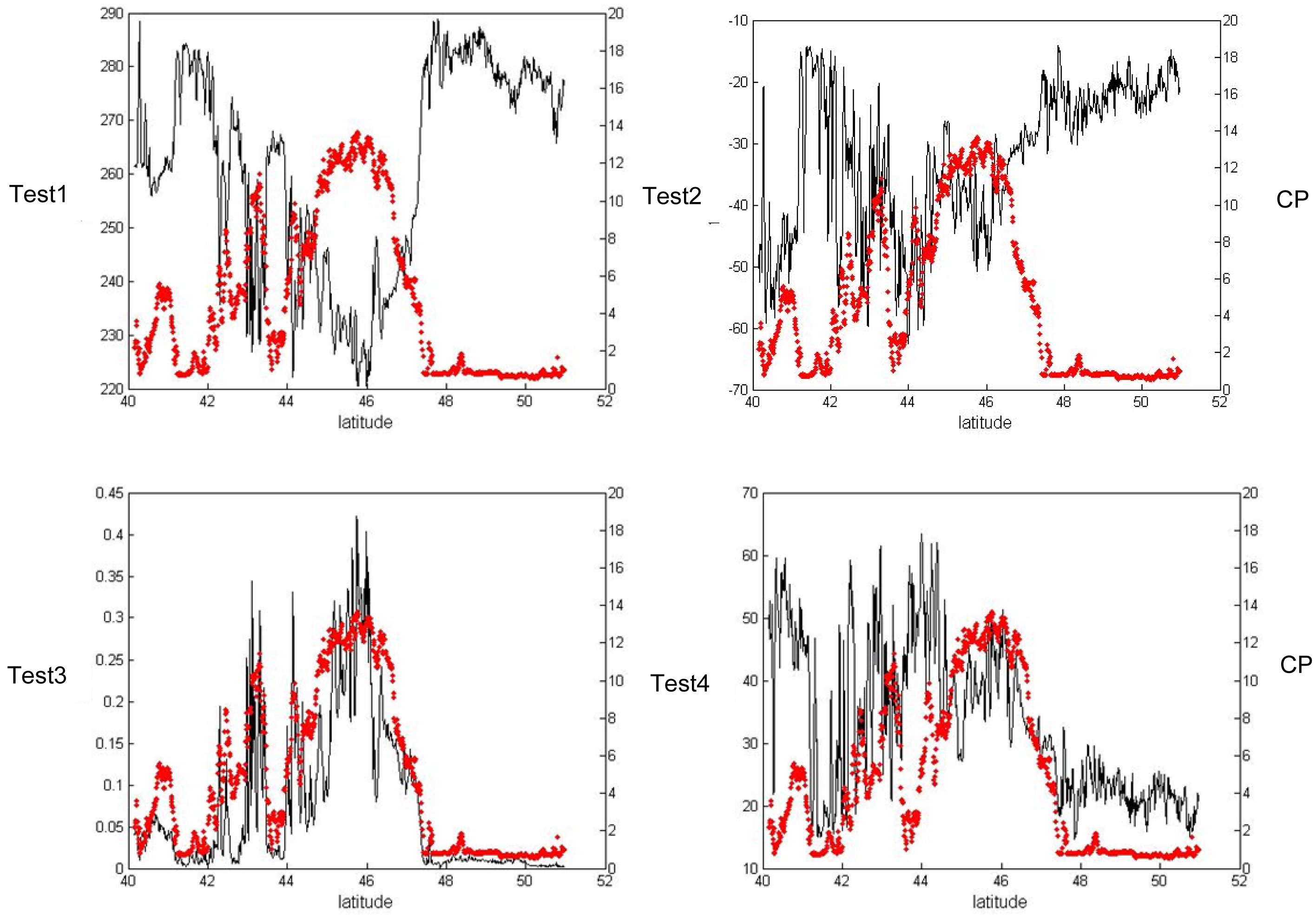
A comparison among the different tests and the CloudSat profile is reported in Figures 2 and 3 for a cloud-free and almost completely cloud-covered day, respectively.
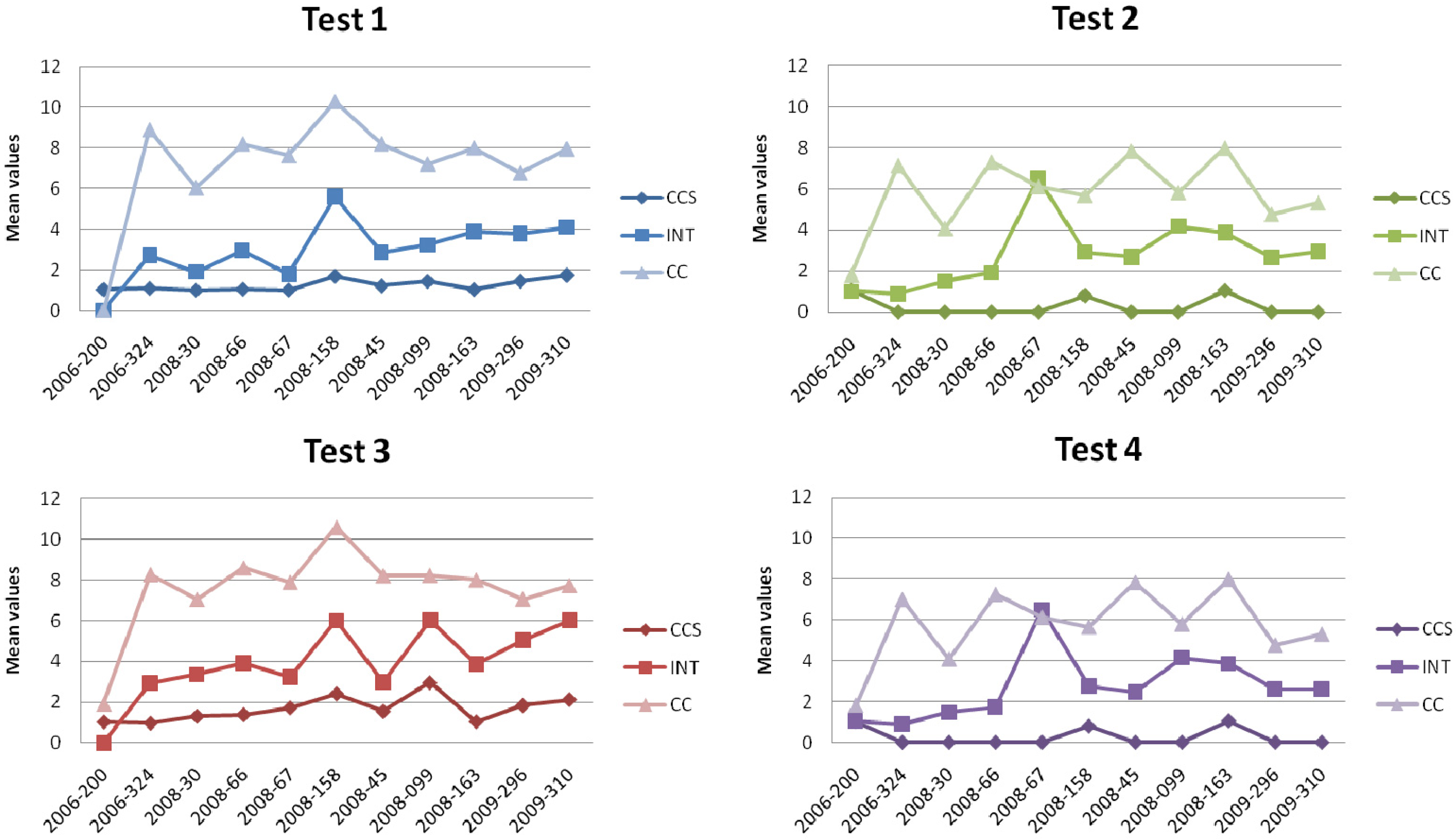
From an initial visual inspection there is a good correlation between the cloud profile and the MODIS test used for the cloud detection. As an example in Figure 3, as the brightness temperature drops below 270 K, the cloud profile values CP increases from 2 up to 12 thus indicating the presence of clouds. The first quantitative assessment was carried out by calculating the mean values of the correspondent cloud profile based on the different thresholds for each test. The comparison is reported in Figure 4, where:
- -
CC represents the mean values of the cloud profile calculated for all the values greater than the thresholds which detect the presence of clouds;
- -
CCS represents the mean values of the cloud profile calculated for all the values lower than the thresholds which detect clear sky;
- -
The intermediate values (INT) indicate all the values between the two thresholds, one for the probable presence of cloudy (PCC) and the other for the probable clear sky (PCS). Regarding the probability, INT includes all values between 0.66 and 0.99.
In the graphs of Figure 4, the classes CC and CCS are well discriminated and this is particularly evident for test 1 and 3, where the mean values for clouds are around 8–10.
For tests 2 and 4, the discrimination between CC and CCS is still present even though the distance between the classes is reduced and the mean values for clouds are between 4 and 8.
The comparison between CloudSat and MODIS for the different tests has also been performed by considering the hit rate calculated with the following formula:
The agreement among the data is also expressed through an index called Hanssen-Kuiper Skill Score (KSS) [21]. This value ranges between −1 and 1 where 0 indicates no coincident event. This index represents the hit rate with respect to a false alarm and remains positive while the hit rate is higher than the false alarm. The KSS index is especially useful when no Gaussian data are analyzed like in the case of clouds. The KSS is calculated in the following way:
- -
a = where both sensors detect clouds;
- -
b = where both sensors detect no clouds;
- -
c = where the first sensor detects clouds and the second one no clouds;
- -
d = where the first sensor detect no clouds and the second one clouds.
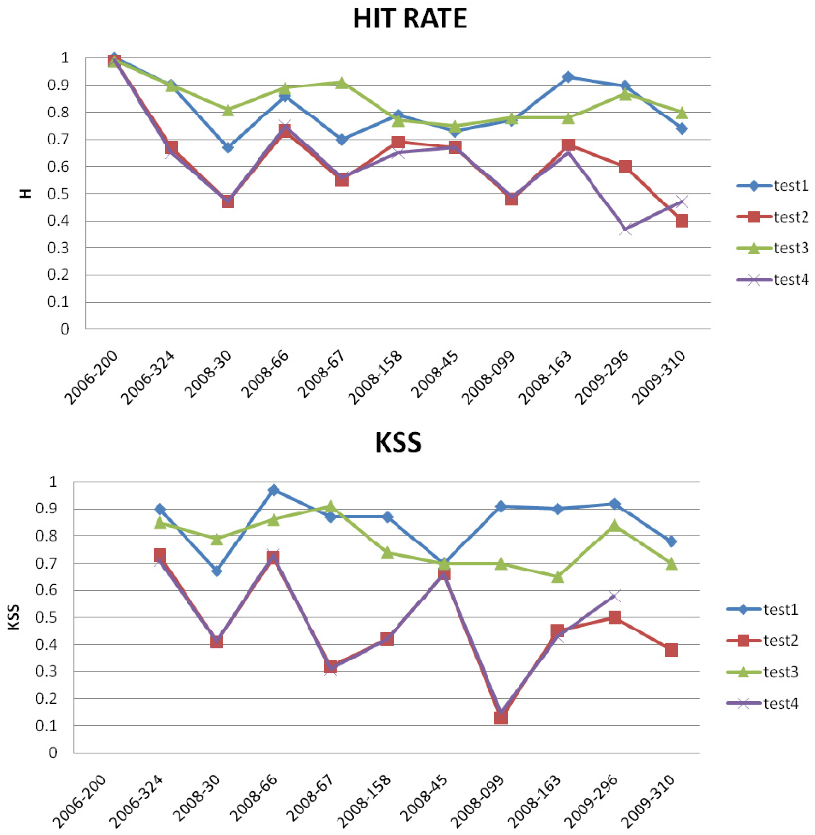
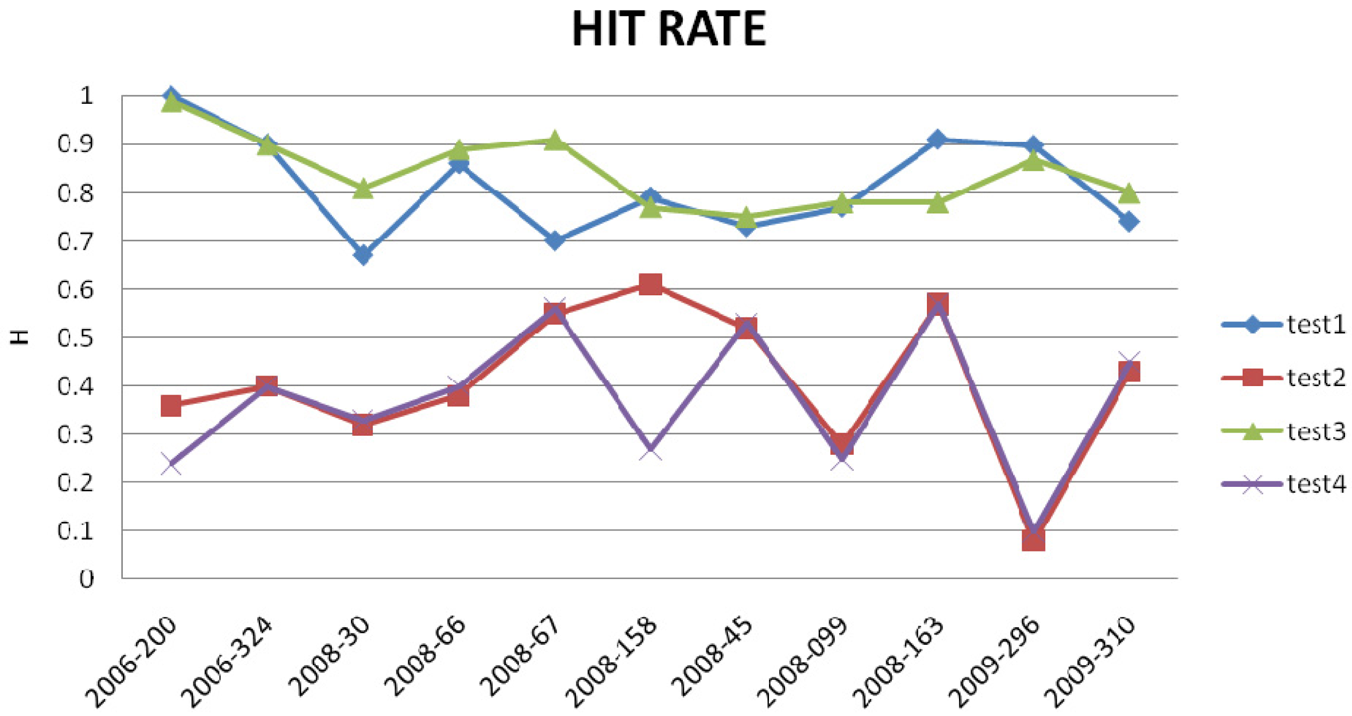
Applying these indices to the previous tests and corresponding cloud profiles, the H index provides good results for tests 1 and 3 with values higher than 0.7, while for the other two tests, the H values are rather low between 0.1 and 0.6 (Figure 5). For KSS index, the values were very low, in most cases equal to zero and are consequently not reported. A possible explanation is given in the following. This behavior can be ascribed to some threshold values which are not appropriate. By observing graphs in Figure 3, the thresholds for clear sky appear far from the thresholds reported for the cloud mask in table 1 that is equal to −9.5 for test 2 and 9.5 for test 4. The latest values can be considered as too conservative thresholds for clear sky. This trend is also verified in most of the other data under investigation. The main effect of these conservative thresholds is to increase the size of the classes “Probably Cloud” and “Probably Not Cloud”.
Furthermore, a very low or zero value for KSS indicates that one class (e.g., the test 1) never hits the correspondent class (CP-Cloud Profile). This behavior means that one threshold is always too low or high to detect points in a class. Analyzing more details in the data, the lack of points is due to the thresholds of no cloud class. As a consequence, the class obtained by using these thresholds is almost always empty. One possible approach is to change these thresholds by following the suggestions provided by the comparison between MODIS and CloudSat profiles.
In fact, from the analysis of the CloudSat data, two new thresholds for clear sky are suggested:
- -
for test 2, values higher than −20 indicate clear sky;
- -
for test 4, values lower than 25 indicate clear sky.
In order to test the effect of these changes, the H and KSS indices have been calculated on the new cloud masks and the results are reported in Figure 6.
The variation introduced in the thresholds determines an increase of the hit rate from 0.4–0.5 to values of 0.5–0.9 for tests 2 and 4. The KSS index has values between 0.3 and 0.7.
The KSS values for tests 2 and 4 are in some cases low. This is due to the fact that the variables of these tests are sensitive to low cloud which is barely detectable by using CloudSat data [9]. In this context the use of CALIPSO data can be of aid.
As an example, these changes in the thresholds have also been verified by considering the effect on the final cloud mask.
The main effect of the changes on the cloud mask in tests 2 and 4 determines a decreasing of the area identified as probably cloud INT.
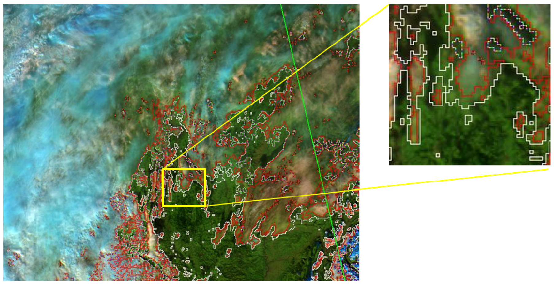
In Figure 7, the comparison with and without the correction is reported, where the old cloud mask is reported in white and the new one in red. The green vector corresponds to the CloudSat track.
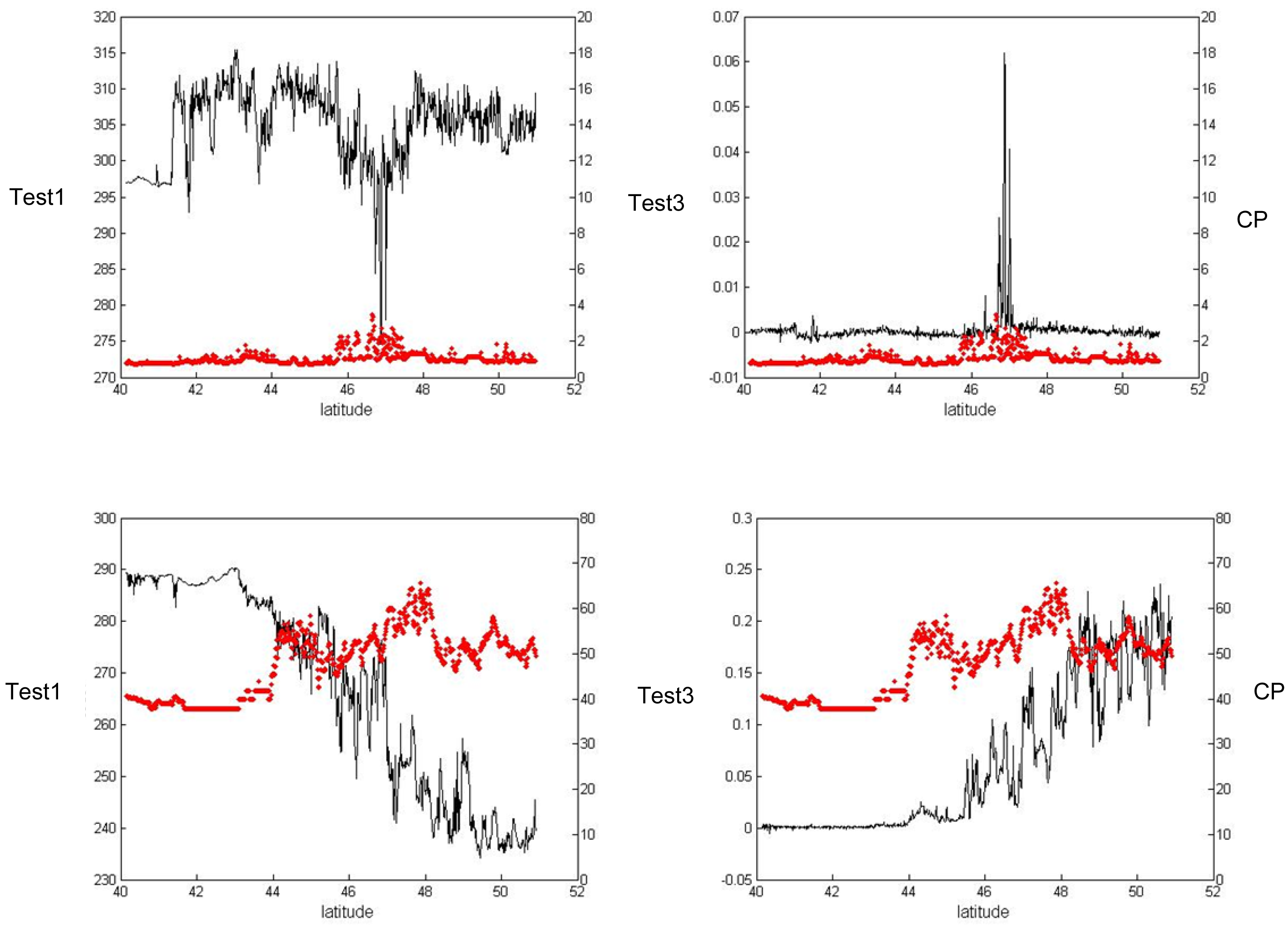
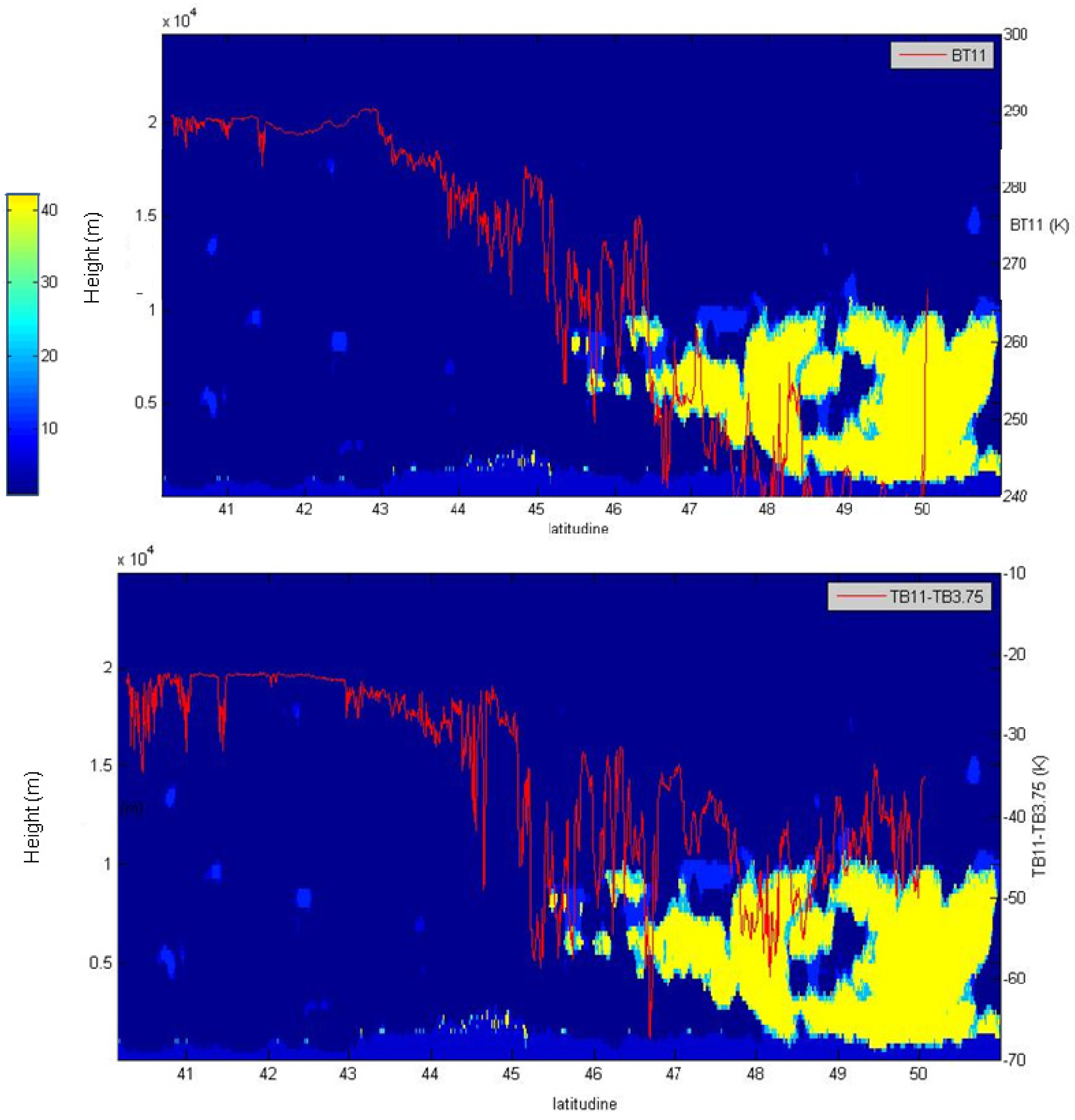
In Figure 8, as for further examples, the bidimensional CloudSat profiles are compared with test 1 values (BT11) and test2 values (BT11-3.75) by considering both the latitude and the height (m).
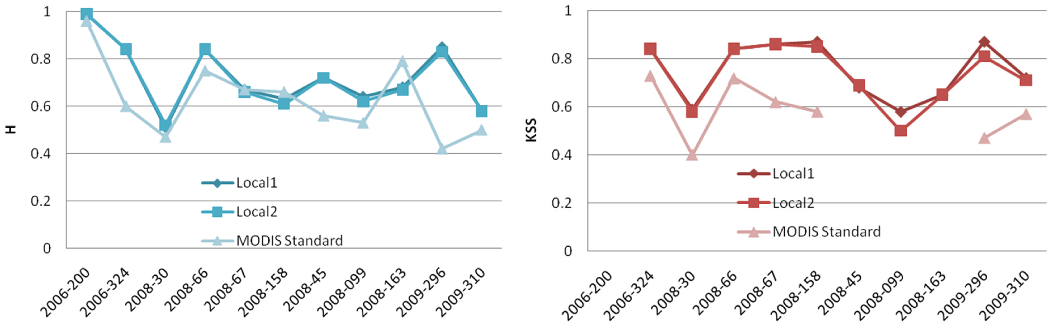
Still looking at the graph with H and KSS rates (Figure 6), there is a special case on 2006-200 characterized by values of H equal to 1 and without any value for KSS. This date corresponds to a completely cloud-free day (see also Figure 2).
As a last example, values from tests 1 and 3 are compared with the cloud profile from the CALIPSO sensor for the date 2006-200 and 2006-324. In both cases, in Figure 9, an agreement is found between the CALIPSO profile and the MODIS tests for the cloud mask. The agreement between the MODIS cloud test and the CALIPSO profile has been evaluated by considering H and KSS indices (Table 2). The missing value corresponds to the KSS value for clear sky day where the no coincidence is found for the cloud class.
To understand the capability of CALIPSO data for detecting low clouds and how they can contribute to the CloudSat data, the comparison MODIS and CALIPSO has been also carried out for the day 2008-030 where the comparison MODIS-CloudSat determines values of H below 0.5 and HSS around 0.4 for both tests 2 and 4. In the case of CALIPSO data, the H values are around 0.83 and the KSS values are around 0.6 for both tests 2 and 4. This preliminary example illustrates the potentialities of CALIPSO with respect to CloudSat data for detecting low clouds. The presence of low clouds was also verified through the use of the product CLOUDCLASS that indicates a 22% of low clouds with respect to the total amount of detected clouds for this date.
As different cloud tests have the capability to detect different cloud types, the final cloud masks have been compared with the CloudSat profile by considering both the initial and the improved thresholds. Furthermore a comparison with the MODIS standard cloud masks colocated with CloudSat profiles has been performed. The results expressed in term of H and KSS indices are reported in Figure 10.
The missing value in the KSS index for the MODIS Standard product indicates that in some classes of values no points to compare are found.
The H and KSS indices of the different cases have been verified through a Wilcoxon significance test. At a 5% level of confidence, the H values in the three cases have been not found to be significantly different. For KSS values, the MODIS standard cloud masks have been found to be significantly different at 5% level of confidence from the local adapted cloud masks. From the analysis derived from these data sets, some considerations can be drawn:
- -
the impact of the new thresholds on the total cloud mask is not relevant because the final mask is derived from a mean of all single tests. Then the presence of an empty class (in the case of the old thresholds) has almost no impact. The effect, however, is evident in some classes such as Probably Clear Sky (PCS);
- -
the local adapted cloud masks seem to perform better with respect to the MODIS standard cloud masks, especially by reducing the false alarm presence;
- -
CloudSat data can also be used to validate the single cloud tests. In these cases, CloudSat shall be sensitive to the cloud type detected by that test.
5. Conclusions
This paper presents a cross-comparison analysis between MODIS cloud mask tests and CloudSat data and provides a rather simple methodology for comparing these different datasets. This is an important aspect because CloudSat data represent a unique case for the validation of the cloud mask algorithm. In fact, in this context, CloudSat data are used as a validation tool for some thresholds for a cloud mask algorithm developed to meet local conditions. The analysis was carried out on 11 scenes for different years and seasons and the results were quantitatively evaluated by using two indices: the hit rate (H) and the Kuiper-Hanssen Skill Score test (KSS). The results indicate a satisfactory agreement between the thresholds set for the different tests and the cloud distribution. For some tests, the accuracy is lower due to the fact that these tests are used to detect low cloud which cannot be easily detected by CloudSat. The comparison of each CloudSat profile with standard MODIS cloud mask indicates that the local adapted thresholds may determine an improved cloud mask. This analysis will be further extended and verified by using larger data sets of CloudSat and CALIPSO images.


| Test | Physical Variables (x) | Threshold for cloud presence | Threshold for clear sky |
|---|---|---|---|
| Test 1 | BT11 | x < 264 | x > 270 |
| Test 2 | BT11−BT3.7 | x < −30 | x > −9.5 |
| Test 3 | ρ1.38 | x > 0.04 | x < 0.03 |
| Test 4 | BT3.7−BT12 | x > 30 | x < 9.5 |
| Test 1 | Test 3 | ||
|---|---|---|---|
| 2006-200 | H | 0.84 | 0.84 |
| KSS | – | 0.84 | |
| 2006-324 | H | 0.77 | 0.82 |
| KSS | 0.67 | 0.70 |
Acknowledgments
This work was carried out in the framework of the project “Nowcasting” (cod. PS_080) supported by regional research funding of Puglia region (Italy).
References
- Liu, Y.; Ackerman, S.A.; Maddux, B.C.; Key, J.R.; Frey, R.A. Errors in cloud detection over the arctic using a satellite imager and implications for observing feedback mechanisms. J. Clim. 2010, 23, 1894–1907. [Google Scholar]
- Ackerman, S.A.; Strabala, K.I.; Menzel, W. P.; Frey, R. A.; Moeller, C. C.; Gumley, L. E.; Baum, B. A.; Schaaf, C.; Riggs, G. Discriminating clear-sky from clouds with MODIS. J. Geophys. Res. 1998, 27, 32141–32157. [Google Scholar]
- Ackerman, S.A.; Strabala, K.I.; Menzel, W.P.; Prey, R.A.; Moeller, C.C.; Gumley, L.E. Discriminating clear-sky from clouds with MODIS. J. Geophys. Res. 1998, 103, 141–157. [Google Scholar]
- Cappelluti, G.; Morea, A.; Notarnicola, C.; Posa, F. Automatic detection of local cloud systems from MODIS data. J. Appl. Meteorol. Clim. 2006, 45, 1056–1072. [Google Scholar]
- Derrien, M.; Farki, B.; Harang, L.; Le Gléau, H.; Noyalet, A.; Pochic, D.; Sairouni, A. Automatic cloud detection applied to NOAA-11/AVHRR imagery. Remote Sens. Environ. 1993, 46, 246–267. [Google Scholar]
- Di Girolamo, P.; Cuomo, V.; Pappalardo, G.; Velotta, R.; Berardi, V. Lidar Validation of Temperature and Water Vapor Satellite Measurements. In Lidar Techniques for Remote Sensing Proceedings of the SPIE; Werner, C., Ed.; SPIE: Bellingham, WA, USA, 1994; Volume 2310, pp. 71–83. [Google Scholar]
- Stephens, G.L.; Vane, D.G.; Boain, R.J.; Mace, G.G.; Sassen, K.; Wang, Z.; Illingworth, A.J.; O'Connor, E.J.; Rossow, W.B.; Durden, S.L.; et al. The CloudSat mission and the A-Train. Bull. Am. Meteorol. Soc. 2002, 83, 1773–1789. [Google Scholar]
- Im, E.; Wu, C.; Durden, S.L. Cloud profiling radar for the CloudSat mission. Proc. Int. Geosci. Remote Sens. Symp. 2007, 5061–5064. [Google Scholar]
- Marchand, R.; Mace, G.G.; Ackerman, T.; Stephens, G. Hydrometeor detection using CloudSat—an Earth-orbiting 94-GHz cloud radar. J. Atmos. Ocean. Technol. 2008, 25, 519–533. [Google Scholar]
- Jin, X.; Hanesiak, J.M.; Barber, D.G. Time series of daily averaged cloud fractions over land fast first-year sea ice from multiple data sources. J. Appl. Meteorol. Clim. 2007, 46, 1818–1827. [Google Scholar]
- Holz, R.E.; Ackerman, S.A.; Nagle, F.W.; Frey, R.; Dutcher, S.; Kuehn, R.E.; Vaughan, M.A.; Baum, B. Global Moderate Resolution Imaging Spectroradiometer (MODIS) cloud detection and height evaluation using CALIOP. J. Geophys. Res. Atmos. 2008, 113, D00A19. [Google Scholar]
- Liu, Y.; Key, J.R.; Frey, R.A.; Ackerman, S.A.; Menzel, W.P. Nighttime polar cloud detection with MODIS. Remote Sens. Environ. 2004, 92, 181–194. [Google Scholar]
- Minnis, P.; Sun_Mack, S.; Yi, Y.; Chen, Y.; Yost, C.; Gibson, S.; Chang, F.; Trepte, C.A.; Wielicki, B.A. Evaluation of CERES-MODIS Cloud Properties Using CALIPSO and CloudSat Data. ATrain-Lille 07 Symposium, Lille France, October, 22–25; 2007. [Google Scholar]
- Frey, R.A.; Ackerman, S.A.; Liu, Y.; Strabala, K.I.; Zhang, H.; Key, J.R.; Wang, X. Cloud detection with MODIS. Part I: Improvements in the MODIS cloud mask for collection 5. J. Atmos. Ocean. Technol. 2008, 25, 1057–1072. [Google Scholar]
- LAADS Web Version 4 Homepage. Available online: http://ladsweb.nascom.nasa.gov/ (accessed on 1 February 2009).
- MODIS Data Homepage. Available online: http://nsidc.org/data/modis/order_data.html (accessed on 1 February 2009).
- CloudSat Data Processing Center Homepage. Available online: http://cloudsat.cira.colostate.edu (accessed on 1 February 2009).
- Di Rosa, D.; Notarnicola, C.; Posa, F. Cross-Comparison and Validation of MODIS AQUA Cloud Mask by Using CLOUDSAT and CALIPSO Datasets. Proceedings of Igarss'09, Cape Town, South Africa, 13–17 July 2009.
- CloudSat Standard Products Handbook; Cooperative Institute for Research in the Atmosphere Colorado State University Fort Collins: Fort Collins, CO, USA, 2007.
- Level 2 Radar-Lidar GEOPROF Product Handbook; Jet Propulsion Laboratory California Institute of Technology Pasadena: Pasadena, CA, USA, 2007.
- Hanssen, A.W.; Kuipers, W.J.A. On the relationship between frequency of rain and various meteorological parameters. Meded. Verh. 1965, 81, 2–15. [Google Scholar]
© 2011 by the authors; licensee MDPI, Basel, Switzerland. This article is an open access article distributed under the terms and conditions of the Creative Commons Attribution license (http://creativecommons.org/licenses/by/3.0/).
Share and Cite
Notarnicola, C.; Di Rosa, D.; Posa, F. Cross-Comparison of MODIS and CloudSat Data as a Tool to Validate Local Cloud Cover Masks. Atmosphere 2011, 2, 242-255. https://doi.org/10.3390/atmos2030242
Notarnicola C, Di Rosa D, Posa F. Cross-Comparison of MODIS and CloudSat Data as a Tool to Validate Local Cloud Cover Masks. Atmosphere. 2011; 2(3):242-255. https://doi.org/10.3390/atmos2030242
Chicago/Turabian StyleNotarnicola, Claudia, Daniela Di Rosa, and Francesco Posa. 2011. "Cross-Comparison of MODIS and CloudSat Data as a Tool to Validate Local Cloud Cover Masks" Atmosphere 2, no. 3: 242-255. https://doi.org/10.3390/atmos2030242