An Ensemble of Arctic Simulations of the AOE-2001 Field Experiment

Abstract
: An ensemble of model runs with the COAMPS© regional model is compared to observations in the central Arctic for August 2001 from the Arctic Ocean Experiment 2001 (AOE-2001). The results are from a 6-km horizontal resolution 2nd, inner, nest of the model while the outermost model domain covers the pan-Arctic region, including the marginal ice zone and some of the land areas around the Arctic Ocean. Sea surface temperature and ice cover were prescribed from satellite data while sea-ice surface properties were modeled with an energy balance model, assuming a constant ice thickness. Five ensemble members were generated by altering the initialization time for the innermost nest, the surface roughness and the turbulent mixing scheme for clouds. The large size of the outer domain means that the model simulations have substantial deviations from the observations at synoptic-scale time scales. Therefore the evaluation focuses on statistical measures, rather than in details of individual ensemble member performance as compared directly to observations. In this context, the ensemble members are surprisingly similar even though details differ significantly. The ensemble average results features two main systematic problems: a consistent temperature bias, with too low temperatures below 2–3 km and slightly high temperatures through the rest of the troposphere, and a significant underestimation of the lowest clouds. In terms of total cloud cover, however, the model produces a realistic result; it is the very lowest clouds that are essentially missing. The temperature bias initially appears to be related to an interaction between clouds and radiation; the shape of the mean radiative heating-rate profile is very similar to that of the temperature bias. The lack of the lowest clouds could be due to the too low temperatures in conjunction with a cloud scheme that overestimates the transfer of cloud droplets to ice particles that precipitate. The different terms in the surface energy balance as well as the surface stress has only small systematic errors and are surprisingly consistent between the members.1. Introduction
Arctic climate has received considerable attention in recent decades due to the apparent enhanced sensitivity at northern hemisphere high latitudes to anthropogenic climate change, as compared to the global average [1,2]. The ACIA (Arctic Climate Impact Assessment) report concludes that temperatures north of 60 °N increased by 0.4 °C per decade over the period 1966 to 2003, while the global average temperature increase was about half this value, 0.25 °C decade−1. This fact, that Arctic near-surface temperatures increase more than the global average, has been termed “Arctic amplification” and has captured much interest, e.g., [3-7]. Especially the consequently decreasing perennial sea-ice cover has been discussed and the dramatic loss of summer sea ice in 2007 generated significant attention, e.g., [8-10]. It seems reasonable to assume that the Arctic amplification is due to some feedback mechanism(s). Although several candidates have been suggested, mechanisms responsible for the Arctic amplification remain elusive: the ice-albedo feedback [11]; long-term loss of ice mass combined with inherent climate variability [12] and changes in the large-scale atmospheric circulation patterns, e.g., [6,8,13]; radiative forcing due to changes in greenhouse gases [14], clouds [15,16] or both [17,18]; inflow of warm ocean water, e.g., [19,20], or a mixture of some or all of these factors. It is important to note that the amplification is also present in climate change scenarios, although the inter-model spread in the strength of the Arctic amplification is very large [21,22]; likely a manifestation both of a large internal variability and an insufficient description of the feedbacks in the Arctic climate system in the different models.
In the Arctic Ocean pack-ice there is a delicate feedback between the low-level boundary layer clouds present in the boundary layer, the semi-permanent ice-covered Arctic surface and the surface energy balance. In particular, presence of clouds over the Arctic Ocean often leads to surface warming, in contrast to the case over mid-latitude oceans [23,24]. Only for a few weeks in summer do clouds have a cooling effect; this is due to a reduced surface albedo both as ice melts and as melt ponds form on the ice. In summer, the near surface temperature often stays relatively constant over the pack-ice, near zero due to the presence of melting ice [6,24]. The largest warming is thus expected to take place in autumn and winter. However, many of the projected changes in the climate system are related to the changes in the length of the melt season, minimum ice extent and ice thickness, e.g., [25]. Twenty-first century model simulations show that significant reductions in summer ice extent is a likely scenario but reductions in future greenhouse gas emissions can moderate the likelihood of these events [26].
Several studies show that global models often have difficulties in reproducing the current Arctic climate, suffering from severe biases; they are too warm especially in winter, have systematic biases in the surface pressure distributions and a large spread in the surface radiative balance [27-29]. In particular the simulation of clouds is very difficult [30,31]. Some of the AR4-family of models even have an inverted annual cycle in cloud cover, with more clouds in winter and less in summer, in contrast to observations [32]. The modeled surface cloud radiative forcing is not consistent with satellite observations and also displays significant inter-model differences [30]. Practically all models overestimate the magnitudes of the surface sensible and latent heat fluxes, especially of the latter, and although the ensemble averages of surface net radiation are more realistic, the inter-model spread is very large [29]. These problems are reproduced in regional models when comparing to data from the Surface Heat Budget of the Arctic Ocean (SHEBA) experiment [33]; the surface turbulent heat fluxes are from two to four times too large [24] regardless of sign and there are significant biases in the cloud representation [34] resulting in systematic errors in downwelling radiation at the surface [31].
Controlled regional model experiments have been developed in order to improve the description of Arctic climate processes in numerical models. The Arctic Regional Climate Model Intercomparison Project (ARCMIP) [35] aims at comparing regional models in the Arctic and identifying model deficiencies with regards to Arctic sub grid-scale parameterizations and improving the formulation of different physical processes for implementation in global models. The first ARCMIP experiment targeted SHEBA observations on a relatively small domain; the performance of several regional models on a common domain was evaluated against yearlong observations from the SHEBA ice-drift [24,36]. In a following study, Wyser et al. [34] found that the inter-model spread of simulated cloud-cover is very large and that many models do not agree with the observed annual cycle even in terms of monthly model means. Simulated albedo also shows large variability and biases during the melt season. Tjernström et al. [31] concluded from the same experiment that besides being poorly described, clouds were generally too optically thick for shortwave radiation in summer while being to optically thin in winter; the latter problem likely due to a problem with mixed-phase clouds. None of the models generate nearly enough liquid water in winter clouds. Thus, there is a need to improve the parameterizations for key processes that control the surface heat budget in order to improve the simulation of the surface melt season.
This first ARCMIP experiment benefited from the fact that the large scale climate was controlled by the prescribed lateral boundaries from global analyses [36]. However, Rinke et al. [37] demonstrate that uncertainties in the lateral boundary forcing and initialization can generate strong internal model variability for simulations within the pan-Arctic region. They find that the largest variability occurs in autumn/winter. As always in regional modeling there is a trade-off between the size of the regional model domain and the degrees of freedom for the regional model; this relates directly to the possibilities of direct comparison of local observations and simulations. Additionally, in the Arctic, limited observations are available for assimilation in the model providing the lateral boundary conditions for the regional model. Therefore the quality of the boundary conditions likely degrades with latitude. Thus while a large domain gives the regional model more freedom, it also ensures better boundary conditions, while a small domain ensures that the regional model dynamics follow the lateral forcing fields more closely, but the quality of that forcing is likely lower.
The size of the domain is also a consequence of the regional modeling application. The simulations in this paper have their root in a series of studies where COAMPS® was applied to study the transport of di-methyl sulfide (DMS), a trace gas important for formation of cloud condensation nuclei and therefore for the formation of clouds [38]. DMS is emitted by biological processes, mainly in the very productive marginal ice zone (MIZ). The motive was to study how much of the observed variability in DMS concentration can be explained by variability in atmospheric dynamic processes alone [39,40]. Since DMS is formed in the MIZ and transported in over the Arctic Ocean pack ice by the atmosphere the domain must extend through the MIZ and into the open water south of the ice edge; therefore the domain has to be pan-Arctic to cover all possible transport routes.
In situ observations in the Arctic for model comparison are scarce and often have poor temporal and spatial resolutions. Birch et al. [41] compared the results from a mesoscale model (COAMPS®) and a global model, the U.K. Met Office Unified Model (UM), at different resolutions with in situ measurements in the high Arctic from late summer of 2001, during the Arctic Ocean Experiment (AOE-2001) [42]. They report that wind speed, surface pressure and relative humidity fields are reasonable well modeled. COAMPS® underestimated the downward long-wave radiation and overestimated downward shortwave radiation compared to observations at times when there is only low-level clouds present, likely an effect of too little cloud liquid water (see also [31]).
In this study we extend the study from Birch et al. [41]. As in that study, the model simulations were conducted using a nesting technique with a pan-Arctic outer model domain and the innermost high-resolution domain centered at the AOE-2001 ice-drift area for August 2001. To facilitate the evaluation of simulations on such a large outer domain using in situ single-point observations, an ensemble approach is explored. The primary intent of this study is thus to investigate the robustness of the simulated meteorological results but in order to accomplish this, also to explore the potential to evaluate large-domain regional model ensemble simulations using detailed field experiment data. A small ensemble of simulations is therefore generated using different initialization times, sea-ice roughness and altering details in the boundary-layer turbulence description; the simulation evaluated by Birch et al. [41] is one of the members in this ensemble and the additional simulations were set up similarly. The model simulations were thus conducted using a nesting technique with a pan-Arctic outer model domain and the innermost high-resolution domain centered at the AOE-2001 ice-drift area, for August 2001. The manuscript is organized with a brief description of the observations followed by a description of the model experiment in Sections 2 and 3, respectively. The results of the simulations are described in Section 4 and the main results and conclusions are discussed in the 5th and 6th Sections.
2. Observations
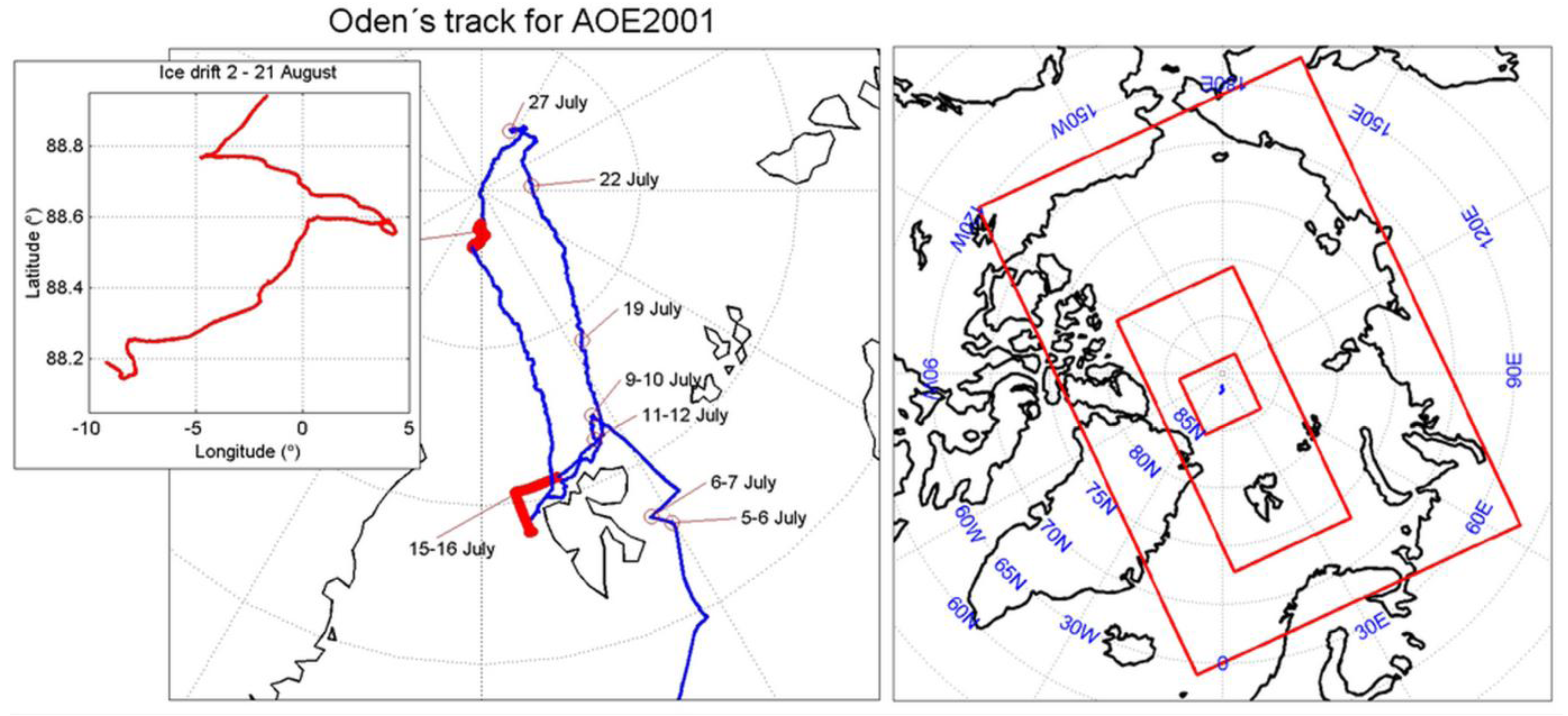
The measurements during the AOE-2001 field campaign were based on the Swedish icebreaker Oden during July and August, 2001 [42]. Continuous atmospheric observations were made during a three week ice-drift with the icebreaker moored to an ice floe drifting from near 89.0 °N, 1.8 °E on 2 August, 2001. After drifting about 150 km in a generally south-western direction the ice-drift phase ended near 88.2 °N, 9.4 °W on 22 August, 2001 (Figure 1).
Observations were carried out both onboard Oden and on stations on the ice. Here we use standard meteorological data from soundings deployed from Oden's helipad, released once every 6 hours during the drift, as well as navigational information collected at the weather station on board. We also use observations from a vertically pointing S-Band Doppler cloud and precipitation radar. The soundings, together with the remote sensing equipment, provide a quasi-continuous vertical-profile record of temperature, relative humidity, wind speed and direction, as well as clouds as a function of altitude. Lidar ceilometer and radar observations were used to access cloud base respectively cloud top heights. Moreover, turbulence and other meteorological variables were sampled by instruments on an 18 m telescopic mast on the ice during the ice drift. For more detailed information of the AOE-2001 equipment and measurement procedures, see [43].
3. Model Set Up and Initialization
We use the Coupled Ocean Atmosphere Mesoscale Prediction System, COAMPS® v3.1.1; a mesoscale model developed at the US Naval Research Laboratory, Monterey [44]. It consists of an atmospheric data assimilation system for initialization of the atmospheric state, a non-hydrostatic atmospheric forecast model and an ocean model; the latter is not used in this study. This model is used both for daily routine weather forecasts and for research. The atmospheric component utilizes a terrain-following σz vertical coordinate with selectable varying grid resolution and allows for a number of user-defined nested grids, with a ratio of 3:1 reduction in grid spacing and time-step between the nests. Simulations were here run with an outer domain at a grid resolution of 54 km, while two smaller nests had grid-point spacing at 18 and 6 km, respectively (Figure 1). The innermost grid was centered on the AOE-2001 drift track while the outer pan-Arctic domain covered the Arctic Ocean, the marginal ice zones and the open ice-free ocean, and parts of surrounding land areas as well as the northern North-Atlantic, thus covering all the main transport pathways into the Arctic Ocean basin.
All grids use 45 vertical model levels, with the first three levels at 3, 10 and 17 m altitude; in total 15 levels were below 550 m while the model top was at 31 km. ERA-40 reanalysis fields at a resolution of 1° × 1° were used for initialization and as 6-hourly lateral boundary forcing at the outer domain. Sea surface temperatures and sea-ice fractions were prescribed from AVHRR (Advanced Very High Resolution Radiometer) and SSMI (Special Sensor Microwave Imager) satellite observations, respectively. The model uses a thermodynamic ice model with separate energy budgets for a constant-thickness sea ice with snow on the ice [45]. Thus, the ice and snow temperatures are allowed to respond to changes in surface energy balance, and to snow melt but not to the melting of ice.
The size of the outermost domain is important for the possibility to compare model results with observations. As the domain size increases, so does the degrees of freedom of the model and thus, without being unphysical, the model may develop an “alternative reality”; a different realization of the development of the atmosphere consistent with the lateral boundary conditions that may deviate from the one single realization that happened, the reality. In this study, the size of the outer domain is chosen to cover the entire Arctic Ocean with its surrounding coasts. Due to the size, spatio-temporal detail may be lost but this can be counteracted by improving the quality of the analyzed boundaries that are closer to more routine observations.
Five different model simulations (see Table 1 for details) were started on 1 July, 2001, the start of the expedition, and last until the end of August 2001; the two outer domains was run for the length of the entire expedition. The outer domain was initialized using data from the reanalysis while fields from the domain immediately outside a nested domain were used to initialize that domain. The inner-most 2nd nest (the third domain) was initialized at different times, initially to save computational time. In three of the simulations the inner 2nd nest was initialized on 00UTC on 15 July (R2, R4 & R5; see Table 1) while in two simulations (R1 & R3) the inner-most nest was initialized later, at 00UTC on 1 August.
Two different roughness lengths were used. While the default roughness for sea ice in COAMPS® is set to 1.4 × 10⁻⁵ m, the same as for the open ocean, Persson et al. [46] quote a mean value of 3.1 × 10⁻⁴ m based on SHEBA observations and Tjernström [24] analyzed the AOE-2001 observations and found a higher value, ∼3 × 10⁻³ m with a span from 5 × 10⁻⁵ m to 2 × 10⁻² m somewhat dependent on wind direction, likely due to localized ridging. The two roughness lengths used in this study are 1.4 × 10⁻⁵ m (in R1 & R2) and 3 × 10⁻³ m (R3, R4 & R5) for the ice covered area; one set of two different initialization times with each roughness length. The roughness length is kept constant through the simulations. Finally, the boundary-layer turbulence parameterization in COAMPS® is a version of the 1.5 order closure of “Level 2.5” in the hierarchy of closures defined by Mellor and Yamada [47]. The first four simulations were carried out with a version of this scheme that does not account for the effects of condensation and cloud water on the buoyancy term in the prognostic Turbulent Kinetic Energy (TKE) equation. One run (R5), while otherwise the same as R4, included a more sophisticated scheme where the turbulent mixing is calculated in moist conservative variables. All together, these five runs constitute the small ensemble of runs analyzed in this study.
Using different initial times for the simulations is classical in ensemble member generation. This essentially expands on the effects of the inherently chaotic nature of the atmosphere. Changes in model physics, on the other hand, expand on the model uncertainty; the fact that no model is perfect and parameters in models are inherently uncertain. Changes in roughness arise from the understanding that this parameter is uncertain and is prescribed different in different models, often different from values estimated from field data. We use both the model's default value and a value that was determined from the observations. Finally, turbulent mixing and clouds is a well known issue in Arctic modeling and is therefore a natural choice. A large ensemble than five would of course have been better; this was constrained by available resources and the fact that this is a pilot study.
4. Results
4.1. Basic Model Performance
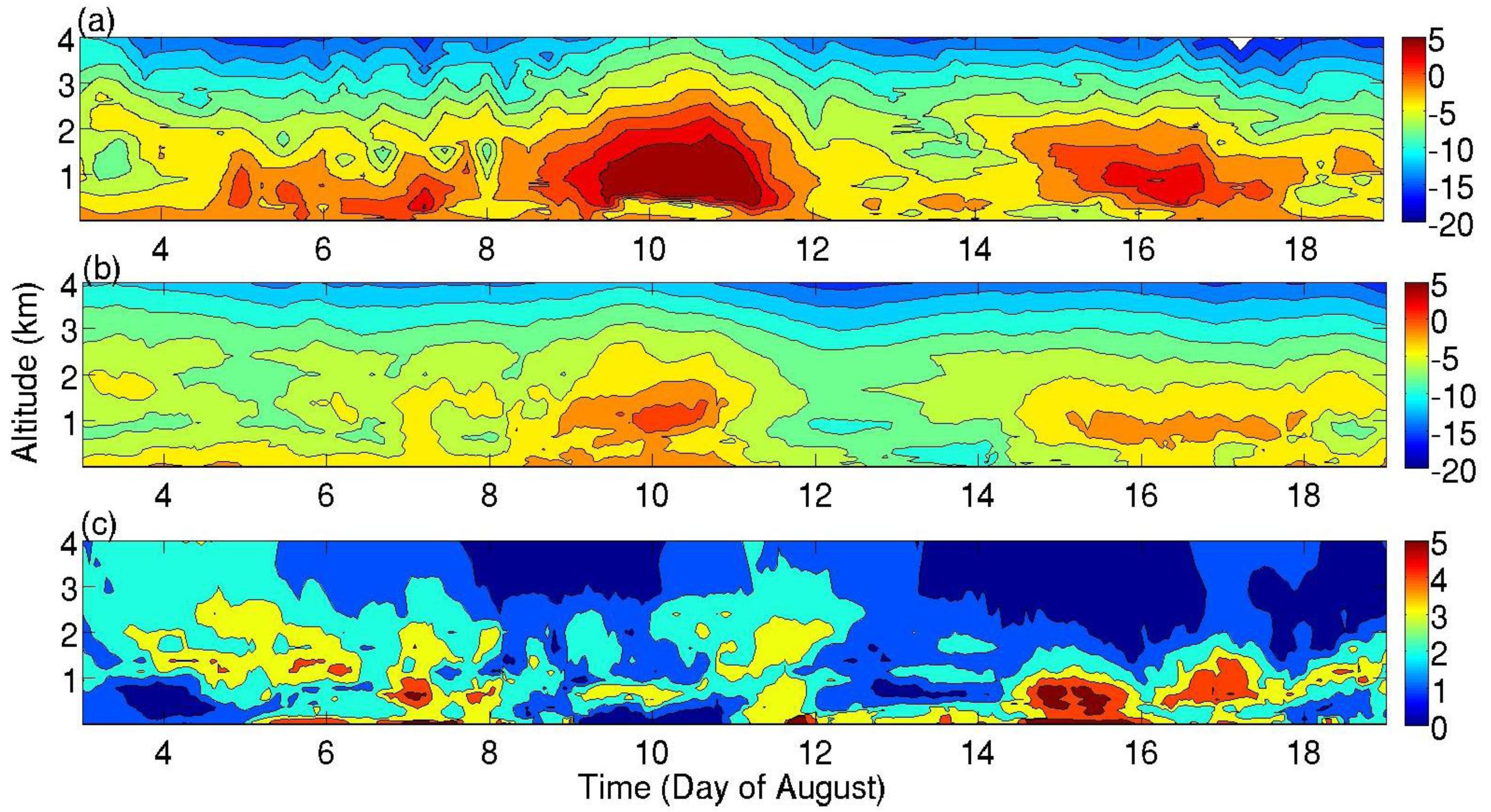
Figures 2–6 illustrate a few of the more prominent features that characterized the AOE-2001 ice drift and summarize some of the model results. Figure 2a shows the time-height cross-section of observed temperature from soundings. The most striking features are the two main intrusions of warm air, the first around 9–12 August and the second around 15–18 August. Both were associated with direct transport of air from the open ocean, the Greenland Sea to the south. In both these events, the temperatures around 1 km height (forthwith all heights are given above sea level) reached well above zero; the temperature reached 8 °C at ∼600 m on 11 August which was the highest temperature observed anywhere at any altitude during the expedition [42]. Also seen are a few weaker intrusions earlier in the ice drift, 5–8 August, and colder boundary-layer temperatures, from midday 14 through 15 August. The lower troposphere was almost always near neutral or slightly stably stratified. Inversions frequently occurred, sometimes at the surface but frequently at the boundary layer top (cf. e.g., [24]). The synoptic events, especially early in the period, are associated with enhanced wind speeds aloft and thus a deeper boundary layer forms decreasing the stability in the lower troposphere.
The ensemble average of the model simulations based on hourly model output (Figure 2b) picks up the main features of the observations, the two warm episodes, but at significantly lower temperatures; a cold bias in the model is evident confined to altitude below 3 km. The timing of the first warm event is well captured in the ensemble mean; the second event is less distinct although the total time is also here roughly correct. The model ensemble also picks up a boundary-layer cold period; however, this is colder than in the observations and occurs about two days too early. The inter-model spread (Figure 2c) is low in the free troposphere (>2–3 km). During the first warm event it is also low in the lower troposphere, but is larger during parts of the second. There are also periods of larger ensemble spread close to the surface around 5–8, around 12 and 14–16 August.
Figure 3 shows the near-surface air temperature from the observations on the ice, for the ensemble average and also for the individual model ensemble members. Also shown is the ensemble spread expressed as the ensemble standard deviation. First examining the observations, it is clear that the warm intrusions seen in the soundings are not observed near the surface. Near surface temperatures instead stayed mostly in the range between −2 and 0.5 °C. This is because the measurements were located on an ice flow with melting ice and snow. When the surface thermal forcing is positive, the surface temperature is in principle limited to near 0 °C as long as there is snow (fresh water) on the surface to melt. Similarly, substantial open-ocean surfaces must freeze over before the temperature can fall significantly; the freezing point of saline sea water is close to −2 °C. The air temperature fluctuates in this range until 14 August, when the temperature starts falling reaching ∼−6 °C at around midday 15 August, after which it rapidly goes up again and continues to oscillate between 0 and −2 °C. All the ensemble members except one, (R3), shows a similar behavior, except for when the temperature drops around 14 August, it drops too much in all of the members but R1. The modeled ensemble averaged temperature follow the temperature evolution fairly well but with a cold bias, except during 9–11 August when there is also very little spread between the ensemble members. Before 8 August, one ensemble member (R3) is much colder and after 11 August most ensemble members are far too cold compared with the observations.
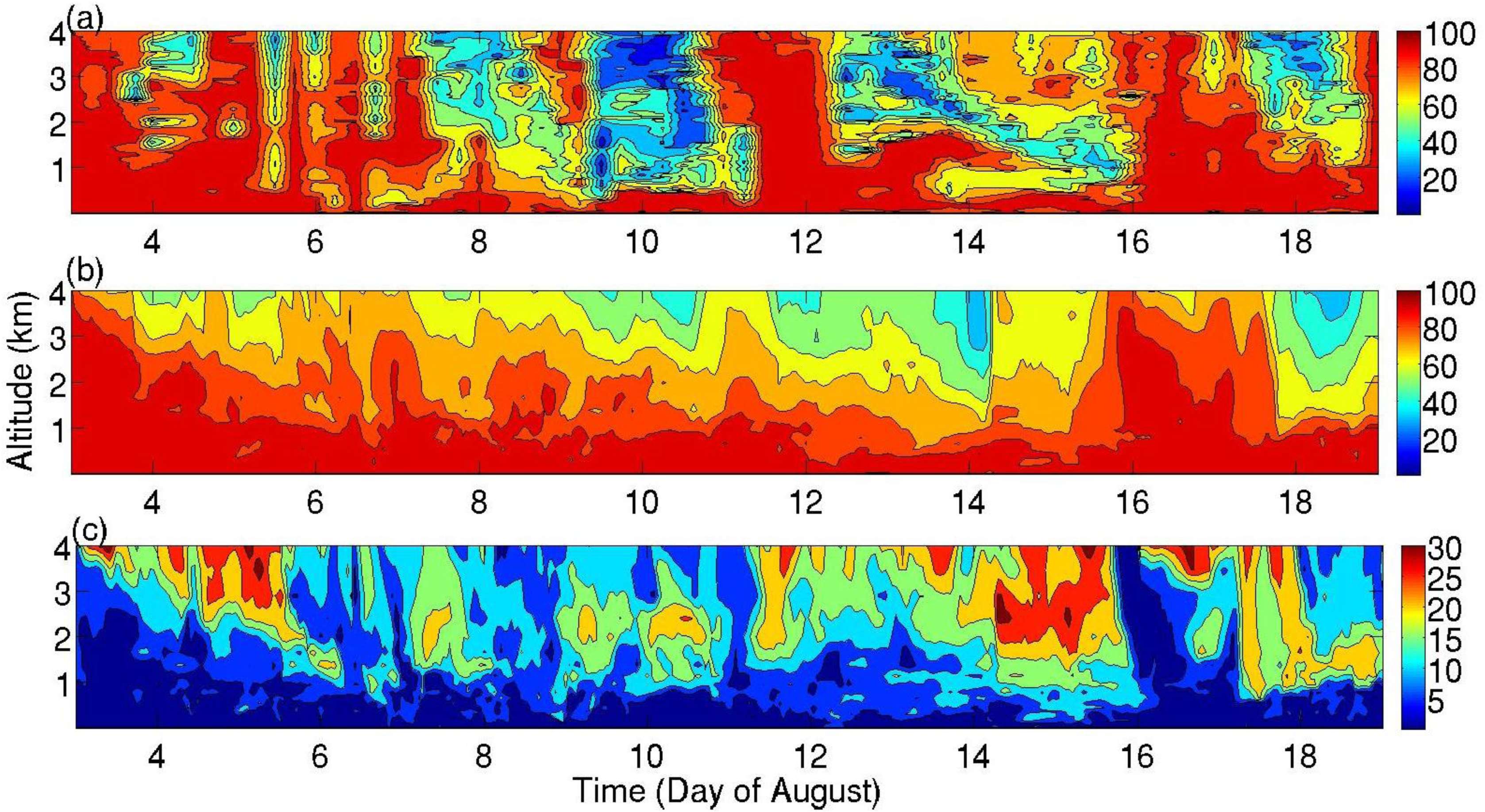
Figure 4 shows time-height cross-sections similar to Figure 2, but for the relative humidity. The lower-troposphere relative humidity remains very high through the whole ice drift (Figure 4a). Tjernström [24] reports near-surface relative humidity during the ice-drift that was consistently high, never falling below 90%. The ensemble average show a deep layer of high relative humidity from the surface to about 3–4 km initially that gradually becomes more shallow with time to about 500 m to 1 km. Passing synoptic weather systems are seen as vertically coherent bands of high relative humidity; several brief ones around 5–7 August and more major systems around 3, 11–12, 16–17 and 19 August. Between some of these, the observed free troposphere relative humidity becomes very low, down to 20% at 3–4 km; see 9–11 and around 13 August.
In a general sense, the ensemble averaged model results (Figure 4b) agrees well with the observations. The model ensemble average again picks up the main features, although the moist layer is somewhat deeper than in the observations. The model also picks up some passing weather systems but not all; one around 12 August seems to be absent or at least much weakened and the one passing 16–17 August arrives earlier than in reality. Although the air aloft is drier in between some of the simulated weather systems it never becomes quite as dry as in the observations, e.g., see around 10 August. The ensemble variability is highest in the free troposphere; this is expected since the relative humidity in the lowest layer is close to 100% all the time in all ensemble members as in the observations, and cannot get any higher. The ensemble variability in the free troposphere is, in contrast to that of temperature, larger and highly coherent in the vertical, and likely tied to the phasing of the weather systems. Higher values are consequently found close to onset and the end of these events. In some cases the agreement between members is better, for example around 6 August and for most of the system passing on 16–17 August.
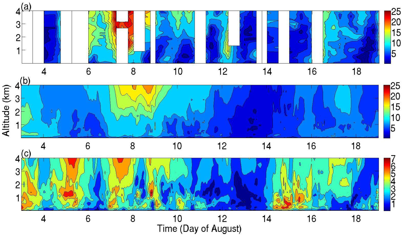
The model performance for the scalar wind speed is poorer than for temperature and relative humidity (Figure 5). On the other hand, there is less temporal coverage in the observations that also appear biased such that wind speed observations are more often missing for high-wind events. For example, the weak wind maximum simulated at the start of the evaluation period hinted in the model (Figure 5b) cannot be evaluated since the wind soundings failed for that time period. There is an indication of an observed wind maximum on 5–6 August that is absent in the model ensemble mean, which is also the case for the maximum around 12 (see above) and 16 August. One of the main events however, around 7–9 August, is captured by the ensemble average, although weaker than in the observations, occurring somewhat later and also lasting longer.
Examining more details (not shown) it is clear that the most important difference in a larger scale context between the ensemble members is, somewhat surprisingly, due to the start time for the inner nest; recall that the outermost domain is the same for all runs. Given the size of the innermost nest (see Figure 1b) one would have expected it to be “flushed through” by the boundary conditions from the outer nests much faster than the differences in initialization time, unless a weather situation develops with small fluxes in or out of the innermost domain, in which case the internal variability might be larger. In the ARCMIP simulations of the SHEBA data [31,34,36,48] the domain was purposely chosen small to ensure that the regional models conform to the imposed larger scale circulation.
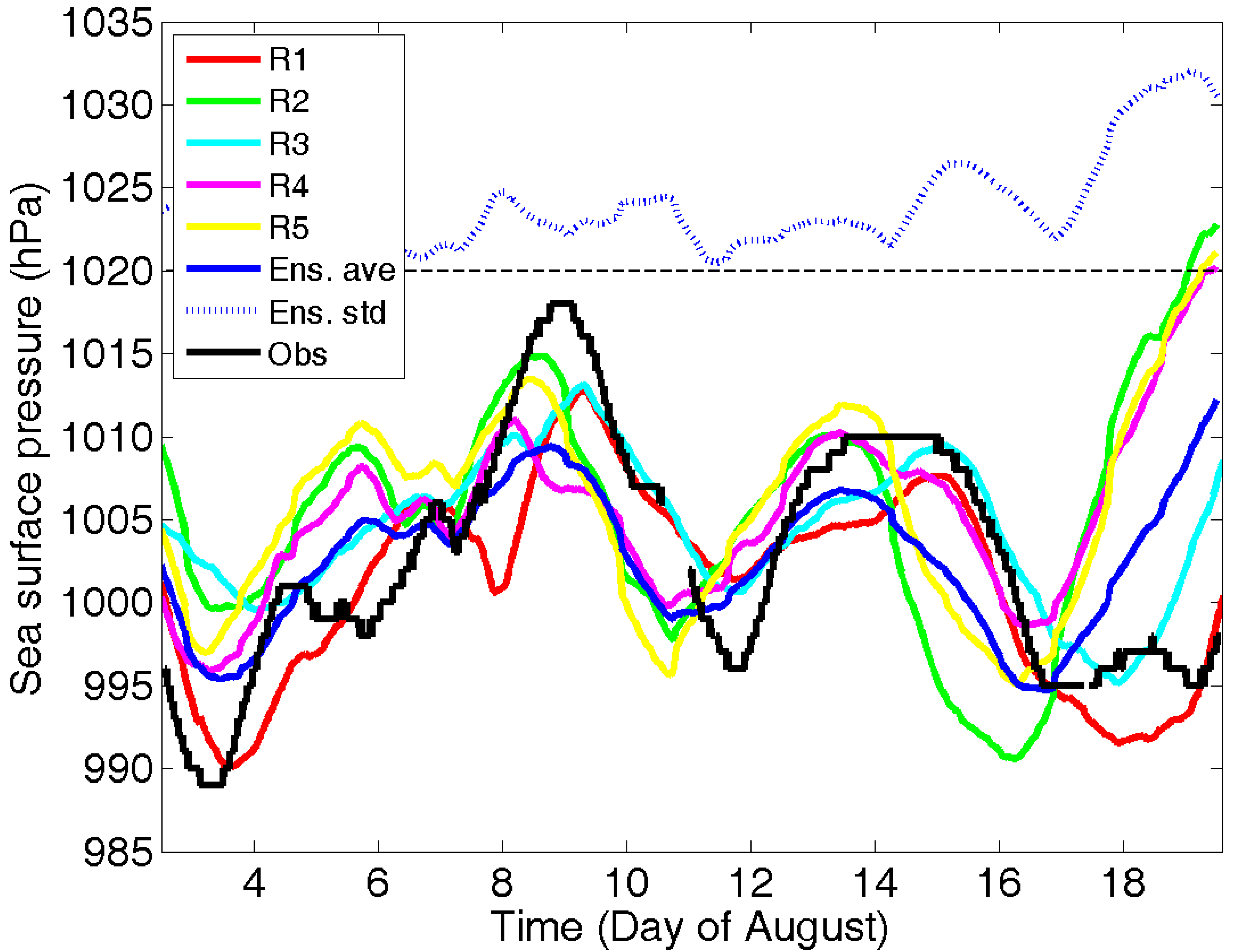
One way to confirm this was a comparison of the simulated and observed surface pressure, e.g., [48]. Figure 6 shows a similar comparison for the present model ensemble. It is clear that the modeled and observed pressures spans about the same values but that the amplitudes of the large-scale pressure variations are smaller in all the ensemble members than in reality. While also being somewhat different in the members, the total variation in the ensemble mean is as much as a factor of two low, and some weaker weather systems are entirely missing, e.g., 6 August. One other significant difference is that the ensemble seems to lead the observations; except for before 5 August, the extremes occur earlier in the model than in the observations. From 17 August there is a significant increase in surface pressure in all ensemble members except R1, that is absent in the observations. The fact that most local maxima and minima in the surface pressure occur roughly simultaneously in all members, except for after 17 August, seems to indicate that these deficiencies are partly inherited by the forcing fields at the lateral boundary and then slightly modified in the nested domains. The reason for the large discrepancies from 17 August and onward is not understood, although it can be noted that the three members most similar to each other, and also the most in error, are the ones that were initialized earlier.
4.2. Systematic Biases
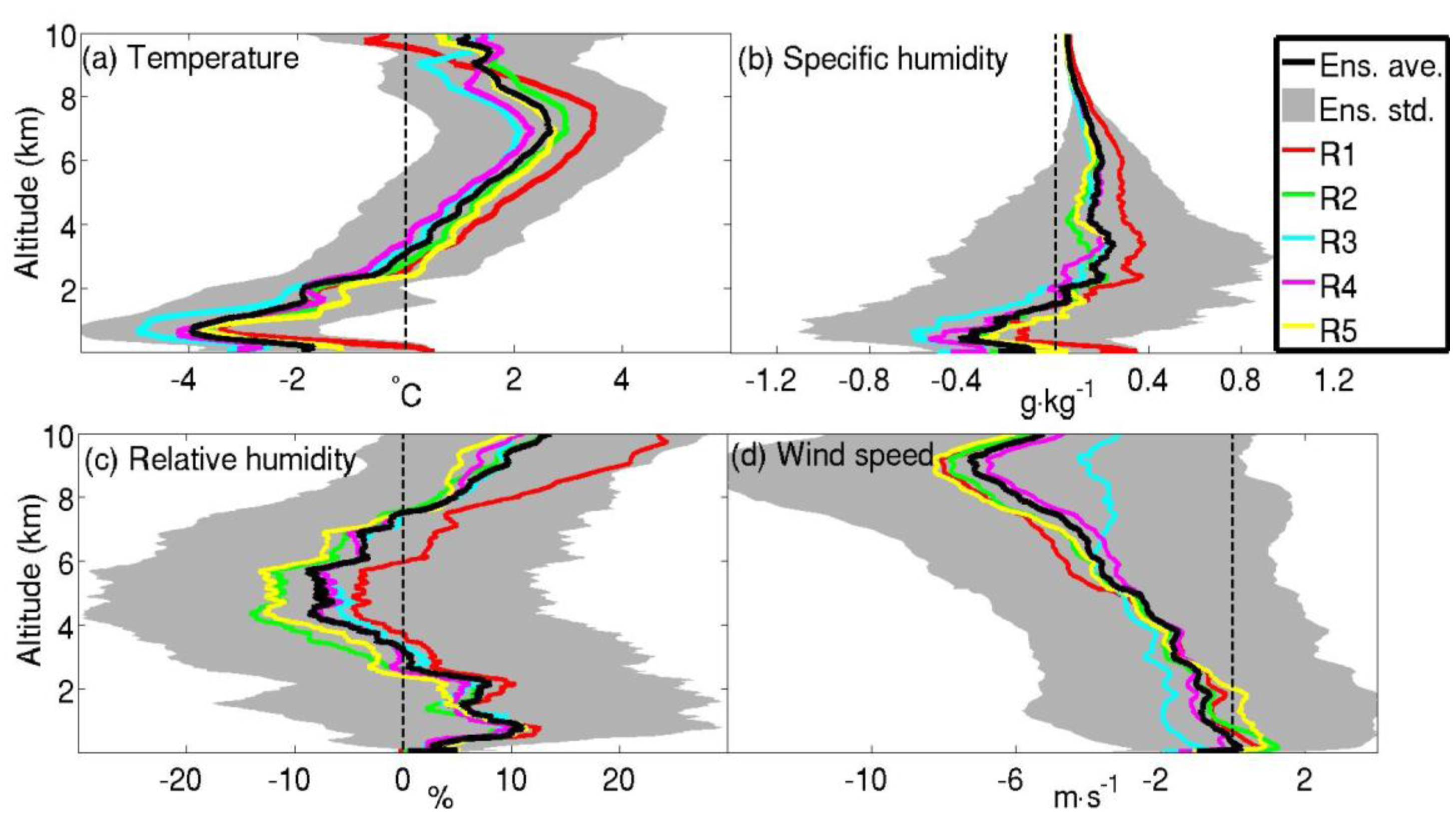
The analysis above indicated some systematic biases in the model manifested by the ensemble average, in contrast to being an effect of stochastic variations between ensemble members. Figure 7 quantifies some of these showing vertical profiles of the ensemble mean bias and its spread for temperature, moisture and scalar wind speed; mean biases for the ensemble members are also shown. The time-height cross-sections of the simulated temperatures (Figure 2b) indicated that the model average tend to produce a cold bias in the lower troposphere. This is confirmed in Figure 7a; below ∼3 km the simulated temperatures are too low. Near the surface the mean temperature bias is ∼−2 °C while the individual member's bias ranges from slightly above zero to ∼−3 °C. This negative bias has a maximum near 700 m of ∼−4 °C; the height is consistent among the ensemble members but the magnitude varies between −3 and −5 °C. This height also corresponds roughly to where the main cloud layer is in the models; see below. The models on average produces too dry conditions in the lower troposphere, below ∼2 km, in terms of specific humidity (Figure 7b). The bias in relative humidity, however, has the opposite indication compared to that in specific humidity; the too cold layer in the lower troposphere is on average 5–10% too moist (Figure 7c). Thus the low-level dry bias in specific humidity (Figure 7b) is a consequence of the temperature bias; an effect of a cold bias and air close to saturation (Figures 2 and 4). In the free troposphere, 2–10 km, these biases are reversed. The temperature is slightly too high and the specific humidity is also too high while the relative humidity is too low, although the ensemble average bias in the latter changes sign in the layer just below the tropopause.
The modeled wind distribution errors are rapidly varying in space and time (Figure 5) but the ensemble average bias is mainly negative and increasing with height, from around zero near the surface to a maximum error of ∼−7 ms−1 close to the tropopause. To the extent that the mean wind shear over the depth of the troposphere is a proxy for the background baroclinicity, this is likely a manifestation of an underestimation of the intensity in the simulated weather systems, also consistent with the too weak variations in surface pressure seen in Figure 6.
There are slight differences in the magnitude of these biases between the different ensemble members but the vertical structure is the same throughout the ensemble. For example, the coldest member overall is R3 with a larger (smaller) cold bias in the lower (free) troposphere. On the other hand, an ensemble mean bias is only statistically significant in temperature in the sense that the ± one standard deviation interval spans zero (no error) through the troposphere for the other three variables; the null hypothesis can thus be rejected only for the temperature. This indicates that at least the bias in temperature is a result of the model itself rather than coming from the model ensemble and that the root cause lies elsewhere in the model physics than in the factors that were altered to generate the ensemble in the first place. The ensemble spread in temperature and relative humidity seems to be relatively height invariant; for specific humidity it varies with the absolute temperature and is thus smaller in the colder conditions aloft. The spread for the simulated winds are also distinctly lower below about 1 km; this is also where the wind bias itself is the smallest.
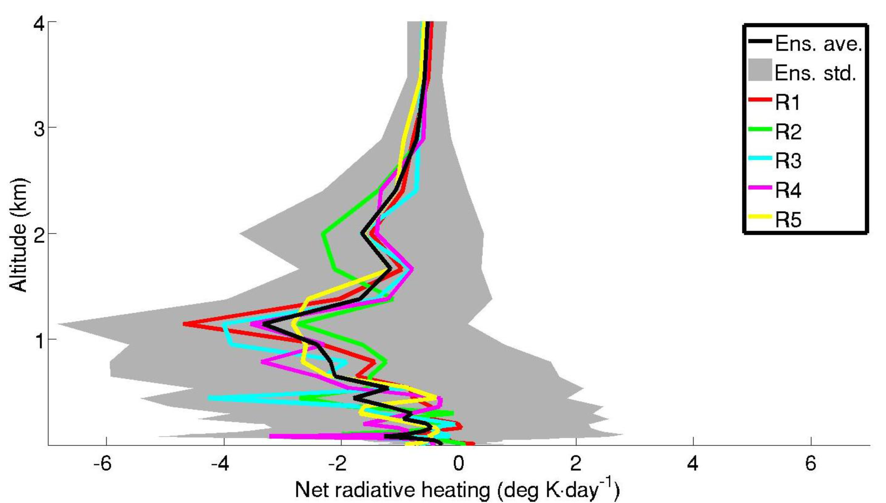
The vertical structure in the temperature bias strongly resembles the vertical structure of the radiative heating/cooling from the model (Figure 8) with a strong cooling in the 500–1,200 m range. The radiative tendencies however remain negative through the troposphere even where the temperature has a warm bias (Figure 7a); quite clearly the cold bias in the low troposphere can be inferred from the radiative tendencies while other processes come into play aloft and warm-air advection may be the dominant process, over-compensating the smaller radiative tendencies.
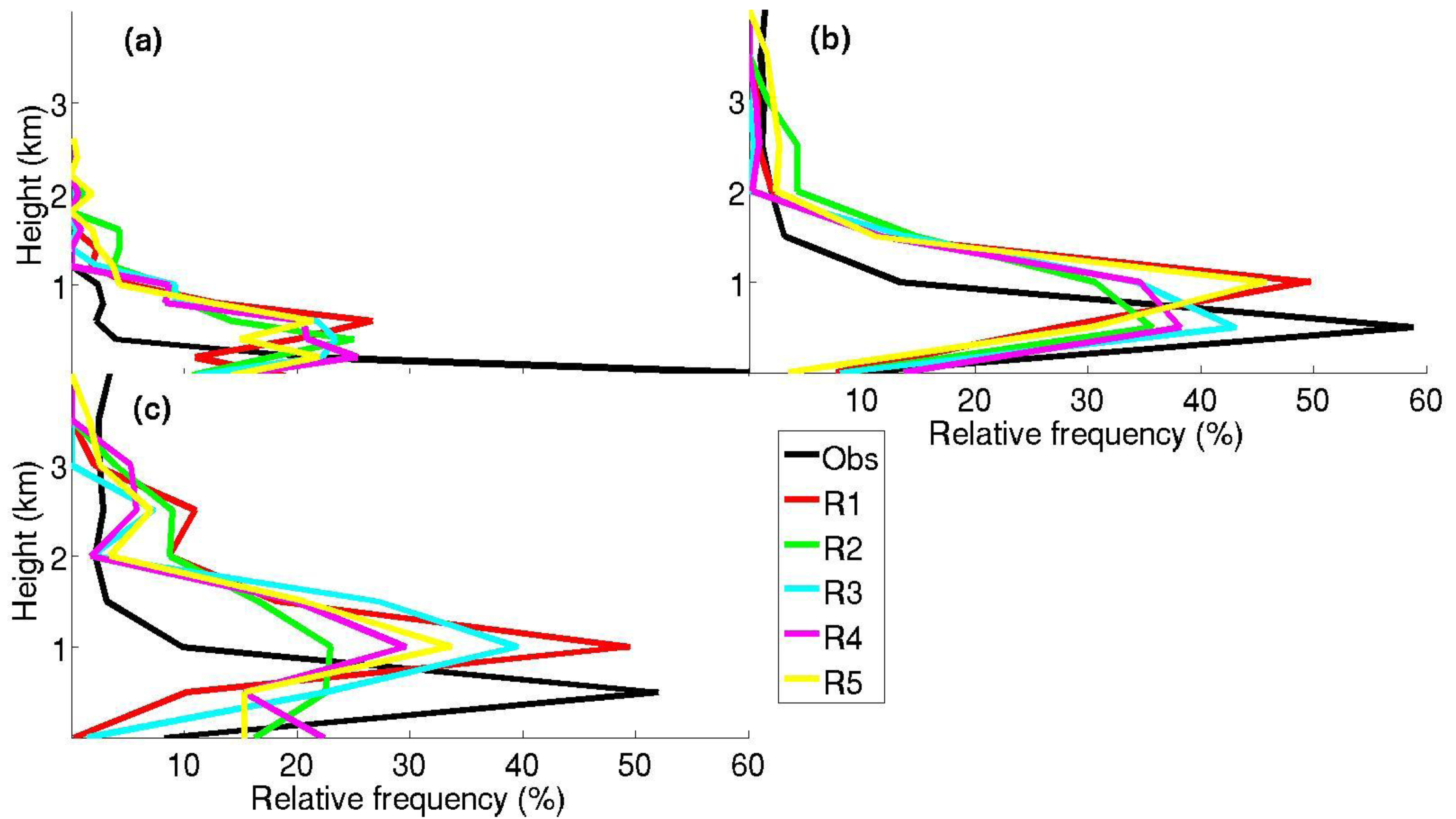
The low-level cold bias and its resemblance to the radiative tendencies points to problems with the interactions between low-level clouds and radiation. The observations indicated a high frequency of occurrence of very low-level clouds [42]; these clouds are to some degree not present in the model. While the observations indicate a predominance of a lowest cloud base close to the surface, below 150 m, all ensemble members have a lowest cloud base between 200 and 800 m (Figure 9a). The lowest cloud top in the observations commonly occurred around 500 m; in the models this is displaced higher to between 800 and 1,200 m (Figure 9b). The statistics for the highest cloud tops is very similar to the lowest cloud top, indicating that single-layer low clouds dominate; for single layer clouds the highest and lowest cloud tops are the same. In the model, the highest cloud tops, compared to the lowest, are displaced somewhat upward. Thus, although the cloud fraction is continuously high, in ensemble members as well as the observations, and the main cloud layer seems to roughly conform to observations, the very lowest clouds with cloud bases typically around 0 to 150 m are less frequent in the model. There is also a tendency, although less so in R5, to confine cloud layers to one or a few grid points in the vertical; the clouds do not seem to mix in the vertical as they did in reality. On the other hand, free troposphere clouds occur slightly more often in the models than in the observations. In conclusion, modeled low-level cloud layers are thinner and displaced at higher altitudes compared with observations while cloud occurrence appears reasonable. Too high and thin clouds reduce the incoming longwave radiation at the surface and thus contribute to the cold bias.
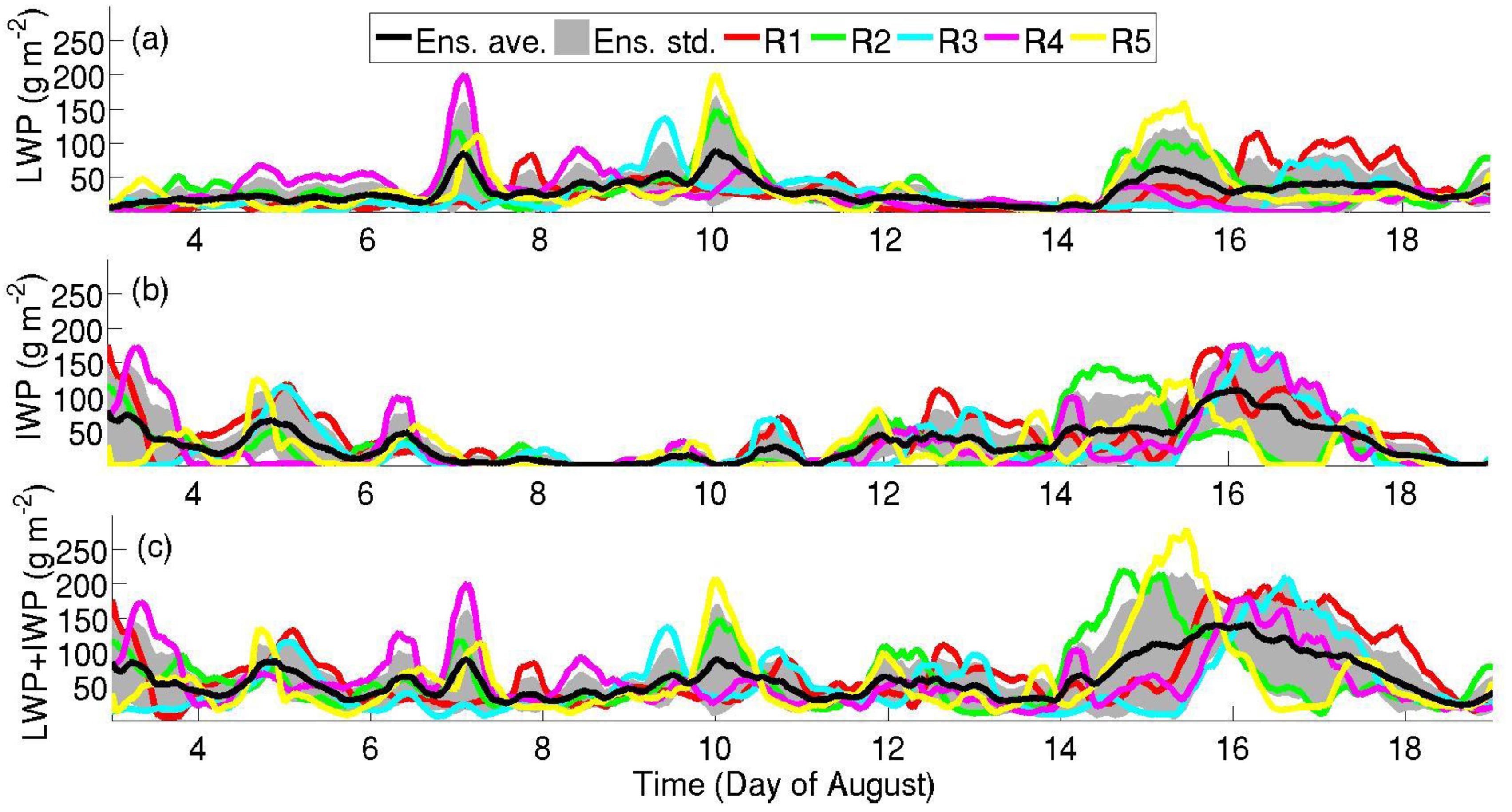
The persistent presence and thickness of clouds can be inferred from Figure 10, showing time series of modeled cloud water paths. First, there is no period of clear-sky conditions (LWP + IWP ∼ 0) seen in the time-series. The ensemble mean cloud water path consist of about half liquid and half ice on average; R3 having considerable lower values (Table 2). The individual ensemble members also mostly agree on high cloud water path in the periods with warm air intrusions, 9–11 and 15–18 August, associated with synoptic weather systems, however, while the first period is dominated by liquid water the latter period has a more even balance between ice and liquid. A few briefer periods with large cloud water path (CWP) associated with synoptic weather also occur. Before 4 August the situation is dominated by ice clouds while the episode around 7 August is dominated by liquid water clouds. Between all these periods the total cloud water path is lower and dominated by liquid water, indicating single-layer low clouds. Unfortunately observations of CWP are not available for comparison, but a comparison between the ensemble members shows a large variability in the exact timing of different weather systems. For example, the LWP peak around 7 August appears only in three of the ensemble members (R2, R4 & R5), which are the three members that were initialized early, and is not present in the other two. Two members (R2 & R5) start the 15–18 August episode earlier while the remainder of the members (R1, R3 & R4) starts it later; the total time for the weather system to pass, however, is similar in all ensemble members. This indicates that both the initialization time and the choice of model physics affect the detailed development in the ensemble members significantly even when the overall development is similar. In between these two periods the LWP is lower, indicating single-layer low clouds.
4.3. Surface Exchange
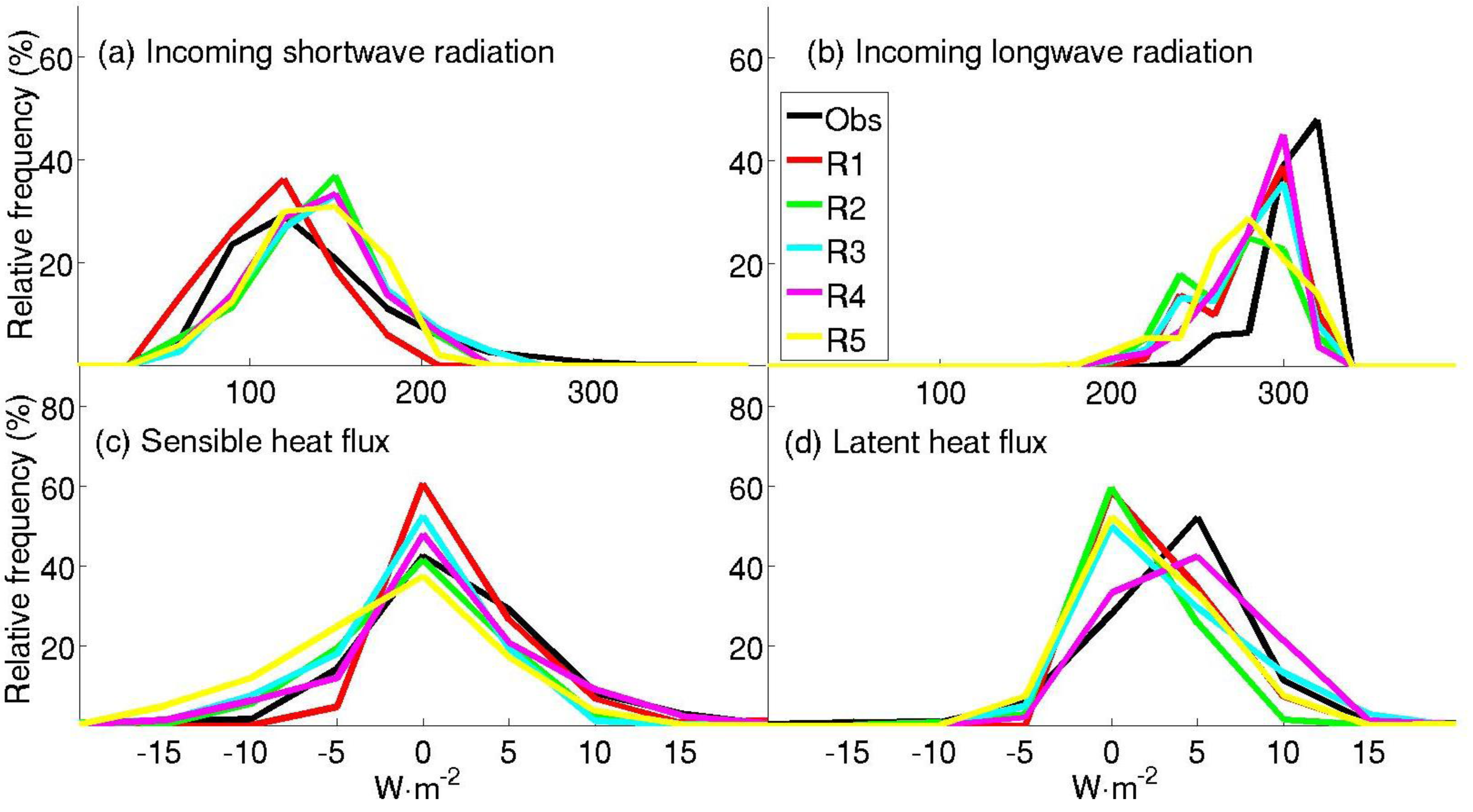
The measurements of turbulent and radiative fluxes at the ice surface allow a comparison of the modeled and observed parameters important for the surface energy balance (Figures 11 and 12).
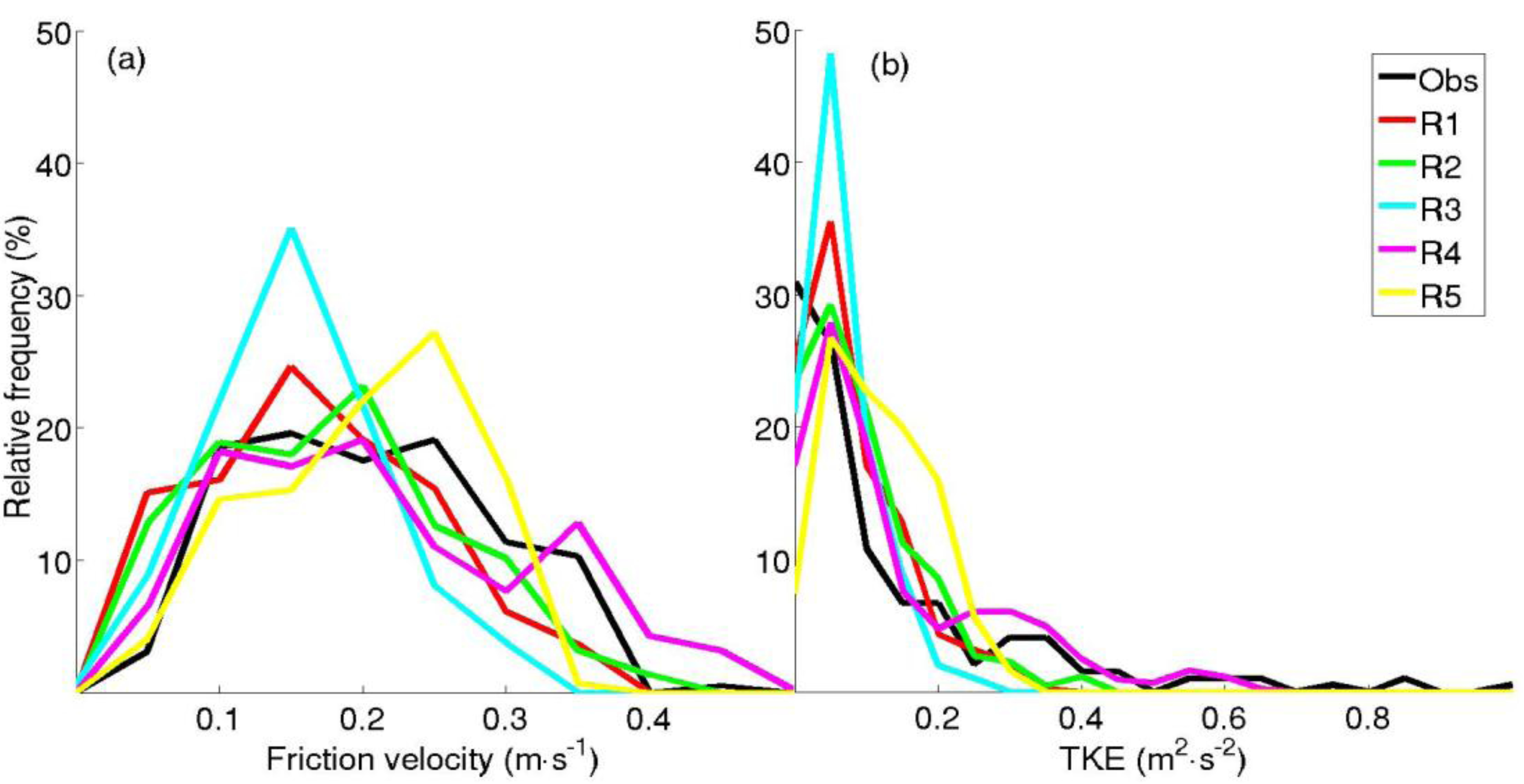
Although the PDF of TKE for all ensemble members peak at a finite non-zero value, while the observation PDF peak at zero, there is in general a good agreement between the models and the observations in a statistical sense (Figure 11b). Also the distributions for surface turbulent momentum fluxes are in good agreement (Figure 11a). This is contrast to the results from the ARCMIP SHEBA experiment, e.g., [48], and also to experience from the GEWEX Boundary Layer Study (GABLS, cf. e.g., [49]). In all these studies the modeled turbulent momentum fluxes were systematically overestimated especially for stably stratified conditions. Surprisingly, there is only a small difference in momentum flux between runs with different surface roughness. The two runs with lower roughness (R1 and R2) show lower TKE values, but have only marginally lower momentum flux. Apparently the near-surface wind speed to some degree adapts and compensates for the lower TKE by a larger wind shear, which in the models together with turbulence determines the momentum flux. On the other hand, R3 has low values of both TKE and momentum flux, which indicate the importance of clouds (see above). As expected the run in which moist processes are included in the TKE equation exhibits the largest TKE and momentum flux.
The corresponding modeled distributions of surface sensible and latent heat exchange show fairly small biases compared with observations (see Figure 12c, d). There is a tendency that modeled latent heat exchange is somewhat small, except for in R4 where the PDF is close to the observed. It should be noted, however, that the observed distribution of latent heat fluxes is derived from a significantly smaller dataset due to a lack of observations for long time periods caused by technical problems in observing water vapor fluxes in this moist environment [24]. The sensible heat flux is quite well captured by the model, with a slight tendency to overestimate negative and underestimate positive fluxes. In general, however, the sensible heat flux is—in a statistical sense—well captured.
Statistics of modeled incoming short-wave radiation at the surface (Figure 12a) show a small positive deviation from the observations, the most significant perhaps being the lack in the model of the observed high-value tail, present in the observations. This indicates that although in a more general sense the models underestimate the clouds, they also miss the few brief periods when clouds disappear entirely or almost entirely (cf. e.g., [41]); thus the cloud fraction is somewhat overestimated (cf. e.g., [41]). Incoming long-wave radiation (Figure 12b) is systematically biased low by the models; the simulations also miss the low-value tail present in the observations for low cloud fractions. The median biases range from ∼−20 to ∼−30 Wm−2; the corresponding negative bias in blackbody temperature is 4–6 °C. A large part of this error could therefore easily be caused by systematic errors in the clouds. A higher cloud base translates directly to a lower cloud-base temperature, thus theoretically this error can be explained by an upward displacement of the clouds compared to reality as is indeed the case here.
5. Discussion
As discussed in the introduction, using a large outer model domain allows much freedom to establish differences in the temporal development at a given point; this makes a direct comparison with single-point observations difficult. Therefore, the majority of the results presented above are discussed in a statistical framework. Given that the detailed observations are only available for roughly a three week period; this also introduces uncertainty by having a short sample. On the other hand, by not assimilating any observations we allow potential differences between simulations time to develop. Below we discuss some of these differences between the model runs confining the discussion to (i) comparisons of pairs of runs with only one parameter changed at the time and (ii) to differences that are statistically significant at the 95% level, using a Student T-test.
The effects of using different initiation times can be assessed by comparing results from R1 with R2 and R3 with R4. These two sets of model experiments are identical except for the higher sea-ice roughness in R3 and R4. From Figure 7 we find that the ensemble members with a longer initiation, R2 and R4, produce a somewhat smaller bias in temperature, humidity and wind speed in the lower troposphere. There are noticeable differences in model performance during the first week of August, where the run with shorter initiation produce very cold surface temperatures associated with cloud-free conditions (compare with Figures 3 and 10). On the other hand, later in the simulation R4 produce an excessive cold period that is not present in the observations. The difference in cloud characteristics between these two runs is small; R4 tends to produce somewhat thicker clouds (see Figure 9) and has higher mean LWP (Table 2). For the surface energy exchange, it seems that model with longer initiation produces a slightly smaller bias in net long-wave flux, probably due to higher average cloud fraction and possibly also due to higher temperatures in the lower troposphere. The surface short-wave flux is also slightly reduced for R4, compared to R3, due to higher effective albedo. Notice also an increase in surface momentum flux and TKE going from R3 to R4, although these differences are just barely statistically significant and correspondingly increased fluxes of sensible and latent energy.
To evaluate the effects of using different values of roughness length over ice, we compare output from R2 and R4. Using a higher roughness length over sea ice tends to produce clouds on a higher average altitude (Figure 9). Even though R2 tend to give a higher average liquid water path (Table 2 and Figure 10), this simulation surprisingly shows less bias in the incoming long-wave radiation compared with R4 (Figure 12b). One explanation for this could be the fact that clouds at a higher altitude are colder and therefore produces less downward long-wave radiation, thus increasing the net surface energy loss, compared to clouds closer to the surface. Furthermore, we find that an ensemble member with higher roughness (R4) produces relatively larger and negative biases in temperature and humidity close to the surface (Figure 7).
Finally, we examine the impact of moist processes by comparing results from R4 and R5. It is clear that the more complex scheme in which moist processes affect the turbulent mixing produces results that significantly reduce the negative temperature and humidity bias in the lower troposphere present in all simulations (Figure 7, see also Figure 3). The wind speed bias in the lower troposphere (<2 km) is positive for R5, in contrast to the other runs, an effect of relatively higher turbulence in the lowest part of the troposphere (Figure 11b).
Considering the clouds in the model we find from Figures 3 and 10 that R5 tends to produce rather short periods with cloud-free conditions. This is the evident when comparing with ensemble members R1 and R3 but also in relation to R4 where the temperature drops excessively in the later part of the simulation period. Notice also that the model run with the moist turbulence scheme also seem to give somewhat deeper cloud layers with a lower cloud base, compared with the other model simulations; this is expected and points to the importance of a more realistic cloud/radiation/turbulence coupling.
6. Summary and Conclusions
Presented here is an evaluation of a small model ensemble of five members for the summer central Arctic Ocean using the COAMPS® regional atmospheric model. The simulations are carried out for the month of August 2001, and observations from the AOE-2001 expedition are used for evaluation. The ensemble is built around three model perturbations, concerning the length of the time of initiation for the inner nest in the regional model, the surface roughness over sea-ice, and the inclusion of moist processes in the turbulent mixing. The ensemble members are otherwise identical; the lateral boundary condition comes from ERA-40, sea surface temperature and ice concentrations from satellite observations, while a thermodynamic ice model with a fixed ice thickness provides the surface boundary conditions over the ice. The simulations were set up with a pan-Arctic outer domain and two nested domain. The aim of this study is to evaluate COAMPS® for Arctic summer conditions while using a pan-Arctic outer model domain and consequently to explore the use of a model ensemble to be able to utilize single-point in situ observations in the evaluation.
While being predictable in principle, the exact atmospheric circulation in a regional model is expected to deviate from reality even in a perfect model; this is a consequence of the chaotic nature of the atmospheric processes. This means that several different synoptic-scale developments may appear, all consistent with the specified boundary conditions and all equally plausible. This freedom grows with the size of the regional model domain. For some applications, the use of a large domain in the Arctic may become unavoidable. For example for regional coupled ocean/ice/atmosphere modeling, there is a need to encapsulate the entire pack-ice area since there is no coupled reanalysis that can provide lateral boundary conditions for the ice and the ocean. Another example is for estimating long-range transport of trace-gas constituents, such as that of di-methyl sulfide from the marginal ice zone and in over the pack ice (e.g., [39,50]); this application necessitated the large outer domain used here, thereby enhancing this freedom for the model compared with previous studies, e.g., [31,48], and thus complicating a direct evaluation against in situ observations at a single location. To alleviate this problem, most of the evaluations described here are performed in a statistical framework. Comparisons are discussed either in terms of differences between the model ensemble and the observations or comparing individual model ensemble members to each other rather than comparing any single model directly to the corresponding observations on a point-by-point basis. The use of an ensemble of models and evaluating against in situ data is shown to provide useful information about the numerical models abilities and discrepancies that would have been difficult to ascertain from a similar evaluation using just one model run. It should be noticed here that, for example, previous evaluations within the ARCMIP framework were also ensembles but consisting of several different models run in a single-run configuration; this also provides useful information but of a different kind. The optimal way of designing a model ensemble, however, remains to be determined.
In terms of model deficiencies, the two largest problems appearing in all ensembles members are the systematic temperature biases and a relative lack of low clouds. There is also a significant bias in the specific moisture which we interpret as a direct consequence of the temperature bias, at least in the lower troposphere. The systematic temperature bias, with a cold bias in the lowest ∼2−3 km and a weaker warm bias through the rest if the troposphere, seems to originate in interactions between the clouds and radiation processes. The most obvious link between them are a striking similarity between the vertical structure of the mean radiative tendency and that of the temperature bias, in addition to the location of largest negative biases in the layers of the atmosphere that is frequently occupied by clouds—in the model as well as the observations. To some extent this problem is augmented by an apparent lack of vertical mixing in the cloudy layers, manifest in a tendency for clouds to occupy single grid layers and not spread out in the vertical; this is handled somewhat better by the model with a more realistic turbulent mixing scheme including moist processes.
The sign of the temperature bias and the radiative tendencies, however, have opposite signs in the free troposphere, thus here the interaction between the clouds and the radiation cannot explain the whole temperature bias. There also seems to be a systematic underestimation of the intensity of the synoptic-sale weather systems, manifest in the too low bulk wind shear across the troposphere and the too week surface-pressure fluctuations. It is difficult to reconcile these problems using a proven regional forecast model continuously forced at the boundaries by atmospheric reanalyzes from ERA-40. It may thus be that these problems are to some degree inherited from the forcing model, either by systematic problems with the Arctic region or from the coarse spatial resolution of the forcing data.
All members in the ensemble, although to a varying degree, underestimate the amounts of the very lowest clouds, compared to the observations. In terms of the total cloud cover the models agree with the observations in showing a predominantly very cloudy environment. Also in agreement with the observations, most of the modeled clouds appear below 1 km; low clouds thus dominate. However, while the observations show frequent cloud layers between below 100 m and up to ∼800 m, with infrequent deeper clouds up to several kilometers associated with weather systems, the different ensemble members have lowest cloud bases spanning from 200–700 m and cloud tops most often between 800 and 1,100 m; the model also more often have cloud systems with cloud tops in the 1–3 km height range. The low cloud layers are thus present in all ensemble members but are often thinner and almost always at a somewhat higher altitude. It is somewhat puzzling that the lowest level clouds are essentially entirely absent in all members while the relative humidity in this layer is in fact overestimated.
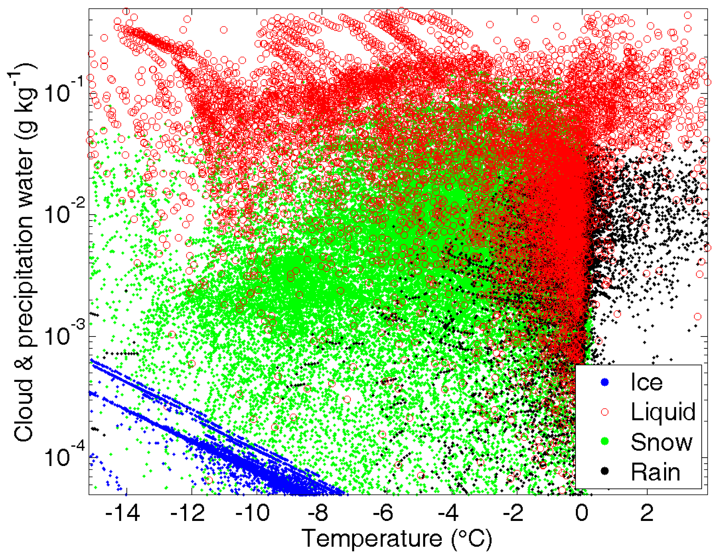
A possible interpretation can be based on three specifics; most are illustrated in Figure 13:
Clouds are most frequent in the warmest (lowest) layer of the troposphere (cf. e.g., Figure 9);
None of the simulations seems to capture mixed-phase in the sense that liquid and ice cloud water never share the same grid points;
Examining the cloud water, frozen or liquid, as a function of temperature there appears to be an “excluded zone” in temperature/cloud-water space in which neither forms of cloud water appears. Moreover, this “gap” spans a large region of realistic low-level liquid cloud water contents at temperatures in this boundary layer, roughly −1 °C > T > −10 °C and liquid water content <0.05 g kg−1.
A possible reason for the lack of low clouds in this “gap” could therefore be that cloud liquid water rapidly undergoes transformation to frozen precipitation and falls out, the Bergeron-Findeisen process, thereby eliminating the cloud. This is supported by the fact that much of the modeled snow mixing ratios are found in this gap, with a significant overlap with liquid cloud water; very few cases of snow mixing ratio is found overlapping with cloud ice.
Somewhat surprisingly, all ensemble members have realistic TKE and momentum fluxes at the surface. These are in a statistical sense very similar between the ensemble members, even for those with very different surface roughness over sea-ice, and agree well with the observations. Also, the turbulent surface heat fluxes are well described. There is a slight tendency that the heat fluxes have too large magnitudes, regardless of sign; both are small. All ensembles members have systematic biases in incoming radiation at the surface, overestimating the shortwave component and an underestimating the longwave component, consistent with the underestimation of low clouds. Both distributions also lack high/low-value tails, seen in the observations for clear-sky conditions.
In summary, with the exception of the significant temperature bias and a systematic lack of the very lowest clouds, the model ensemble in a statistical sense reproduces observations from the central Arctic Ocean during August 2001 when the AOE-2001 expedition provided detailed observation taken over the perennial central Arctic sea ice. In particular, the important energy fluxes at the surface are in good agreement with the observations. A lack of high wind speeds in the upper troposphere and too low amplitude in the surface-pressure variability on synoptic time scales indicate an underestimation of the baroclinic activity manifested by weather systems. The time-resolved details of the observations are in some, but not all, respects reproduced by the model ensemble members and differences both between the ensemble members and between the ensemble average and the observations can be explained by the relatively large pan-Arctic model domain allowing large freedom for the model to develop its own synoptic scale developments while still conforming to the lateral boundary conditions. The results illustrate how a single-model regional ensemble may be utilized to evaluate regional model performance using in situ observations.


| Model run | Initialization (refers to innermost nest) | Roughness length (m) | Mixing scheme |
|---|---|---|---|
| R1 | 1 August | 1.4 × 10⁻⁵ | Dry |
| R2 | 15 July | 1.4 × 10⁻⁵ | Dry |
| R3 | 1 August | 3 × 10⁻³ | Dry |
| R4 | 15 July | 3 × 10⁻³ | Dry |
| R5 | 15 July | 3 × 10⁻³ | Moist |
| R1 | R2 | R3 | R4 | R5 | Ens. Ave. | |
|---|---|---|---|---|---|---|
| LWP (gm−2) | 26 | 33 | 24 | 26 | 31 | 28 ± 4 |
| IWP (gm−2) | 40 | 34 | 24 | 37 | 32 | 33 ± 6 |
| LWP + IWP (gm−2) | 66 | 67 | 48 | 63 | 63 | 61 ± 8 |
Acknowledgments
This work was supported by the Bert Bolin Center for Climate Research at Stockholm University. The Bolin Center is funded by FORMAS and the Swedish Research Council as a “Linnaeus Center of Excellence”. Laurent Brodeau assisted in running the model.
References
- ACIA. Impacts of a Warming Arctic, Climate Impacts Assessments; Cambridge University Press: Cambridge, UK, 2004. [Google Scholar]
- IPCC. Climate Change 2007: The Physical Science Basis; Cambridge University Press: Cambridge, UK, 2010. [Google Scholar]
- Serreze, M.C.; Francis, J.A. The arctic amplification debate. Clim. Change 2006, 76, 241–264. [Google Scholar]
- Alexeev, V.A.; Langen, P.L.; Bates, J.R. Polar amplification of surface warming on an aquaplanet in “ghost forcing” experiment without sea ice feedbacks. Clim. Dyn. 2005, 24, 655–666. [Google Scholar]
- Graversen, R.G. Do Changes in the mid-latitude circulation have any impact on the arctic surface air temperature trend? J. Clim. 2006, 19, 5422–5438. [Google Scholar]
- Graversen, R.G.; Mauritsen, T.; Tjernström, M.; Källén, E.; Svensson, G. Vertical structure of recent Arctic warming. Nature 2008, 541, 53–56. [Google Scholar]
- Lu, J.; Cai, M. Quantifying contributions to polar warming amplification in an idealized coupled general circulation model. Clim. Dyn. 2010, 34, 669–687. [Google Scholar]
- Zhang, X.; Sorteberg, A.; Zhang, J.; Gerdes, R.; Comiso, J.C. Recent shifts of atmospheric circulations and rapid changes in Arctic climate system. Geophys. Res. Lett. 2008, 35, L22701. [Google Scholar] [CrossRef]
- Wang, M.; Overland, J.E. A sea ice free summer Arctic within 30 years? Geophys. Res. Lett. 2009, 36, L07502. [Google Scholar] [CrossRef]
- Graversen, R.G.; Mauritsen, T.; Drijfhout, S.; Tjernström, M.; Mårtensson, S. Warm winds from the Pacific caused extensive Arctic sea-ice melt in summer 2007. Clim. Dyn. 2010. [Google Scholar] [CrossRef]
- Perovich, D.K.; Richter-Menge, J.A.; Jones, K.F.; Light, B. Sunlight, water and ice: Extreme Arctic sea ice melt during the summer of 2007. Geophys. Res. Lett. 2008, 35, L11501. [Google Scholar] [CrossRef]
- Overland, J.E. The Cause for Global Warming in the Arctic, Influence of Climate Change on the Changing Arctic and Sub-Arctic Conditions; Springer: Berlin, Germany, 2009; pp. 13–23. [Google Scholar]
- Overland, J.E.; Wang, M.; Salo, S. The recent Arctic warm period. Tellus 2008, 60, 589–597. [Google Scholar]
- Serreze, M.C.; Holland, M.M.; Stroeve, J. Perspectives on the Arctic's shrinking sea-ice cover. Science 2007, 315, 1533–1536. [Google Scholar]
- Liu, Y.; Key, J.R.; Wang, X. The influence of changes in cloud cover on recent surface temperature trends in the Arctic. J. Clim. 2008, 21, 705–715. [Google Scholar]
- Kay, J.E.; L'Ecuyer, T.; Gettelman, A.; Stephens, G.; O'Dell, C. The contribution of cloud and radiation anomalies to the 2007 Arctic sea ice extent minimum. Geophys. Res. Lett. 2008, 35, L08503. [Google Scholar] [CrossRef]
- Francis, J.A.; Hunter, E. Changes in the fabric of the Arctic's greenhouse blanket. Environ. Res. Lett. 2007, 2. [Google Scholar] [CrossRef]
- Graversen, R.G.; Wang, M. Polar amplification in a coupled climate model with locked albedo. Clim. Dyn. 2009, 33, 629–643. [Google Scholar]
- Shimada, K.; Kamoshida, T.; Itoh, M.; Nishino, S.; Carmack, E.; McLaughlin, F.; Zimmermann, S.; Proshutinsky, A. Pacific Ocean inflow: Influence on catastrophic reduction of sea ice cover in the Arctic Ocean. Geophys. Res. Lett. 2006, 33, L08605. [Google Scholar] [CrossRef]
- Polyakov, I.V.; Alexeev, V.A.; Belchansky, G.I.; Dmitrenko, I.A.; Ivanov, V.V.; Kirillov, S.A.; Korablev, A.A.; Steele, M.; Timokhov, L.A.; Yashayaev, I. Arctic ocean freshwater changes over the past 100 years and their causes. J. Clim. 2008, 21, 364–384. [Google Scholar]
- Holland, M.M.; Bitz, C.M. Polar Amplification of climate change in coupled models. Clim. Dym. 2003, 21, 221–232. [Google Scholar]
- Sorteberg, A.; Furevik, T.; Drange, H.; Kvamsto, N.G. Effects of simulated natural variability on Arctic temperature projections. Geophys. Res. Lett. 2005, 32, L18708. [Google Scholar] [CrossRef]
- Intrieri, J.M.; Fairall, C.W.; Shupe, M.D.; Persson, P.O.G.; Andreas, E.L.; Guest, P.S.; Moritz, R.E. An annual cycle of Arctic surface cloud forcing at SHEBA. J. Geophys. Res. 2002, 107, 8039. [Google Scholar] [CrossRef]
- Tjernström, M. The summer Arctic boundary layer during the Arctic Ocean Experiment 2001 (AOE-2001). Boundary-Layer Meteorol. 2005, 117, 5–36. [Google Scholar]
- Markus, T.; Stroeve, J.C.; Miller, J. Recent changes in Arctic sea ice melt onset, freezeup, and melt season length. J. Geophys. Res. 2009, 114, C12024. [Google Scholar] [CrossRef]
- Holland, M.M.; Bitz, C.M.; Tremblay, B. Future abrupt reductions in summer Arctic sea ice. Geophys. Res. Lett. 2006, 33, L23503. [Google Scholar] [CrossRef]
- Walsh, J.E.; Kattsov, W.M.; Chapman, W.L.; Govorkova, V.; Pavlova, T. Comparison of Arctic climate simulated by uncoupled and coupled global models. J. Clim. 2002, 15, 1429–1446. [Google Scholar]
- Chapman, W.L.; Walsh, J.E. Simulations of Arctic temperature and pressure by global coupled models. J. Clim. 2007, 20, 609–632. [Google Scholar]
- Sorteberg, A.; Kattsov, V.; Walsh, J.E.; Pavlova, T. The Arctic surface budget as simulated with the IPCC AR4 AOGCMs. Clim. Dyn. 2007, 29, 131–156. [Google Scholar]
- Karlsson, J.; Svensson, G. The simulation of Arctic clouds and their influence on the winter surface temperature in present-day climate in the CMIP3 multi-model dataset. Clim. Dyn. 2010, 36, 623–635. [Google Scholar] [CrossRef]
- Tjernström, M.; Sedlar, J.; Shupe, M.D. How well do regional climate models reproduce radiation and clouds in the Arctic? An evaluation of ARCMIP simulations. J. Appl. Meteorol. Climatol. 2008, 47, 2405–2422. [Google Scholar]
- Wang, X.; Key, J.R. Arctic surface, cloud, and radiation properties based on the avhrr polar pathfinder dataset. part I: Spatial and temporal characteristics. J. Clim. 2005, 18, 2558–2574. [Google Scholar]
- Uttal, T.; Curry, J.A.; McPhee, M.G.; Perovich, D.K.; Moritz, R.E.; Maslanik, J.A.; Guest, P.S.; Stern, H.L.; Moore, J.A.; Turenne, R.; et al. Surface heat budget of the arctic ocean. Bull. Am. Meteorol. Soc. 2002, 83, 255–275. [Google Scholar]
- Wyser, K.; Jones, C.G.; Du, P.; Girard, E.; Willén, U.; Cassano, J.; Christensen, J.H.; Curry, J.A.; Dethloff, K.; Haugen, J.E.; et al. An evaluation of Arctic cloud and radiation processes during the SHEBA year: simulation results from eight Arctic regional climate models. Clim. Dyn. 2008, 30, 203–223. [Google Scholar]
- Curry, J.A.; Lynch, A.H. Comparing Arctic regional climate models. Eos. Trans. Am. Geophys. Union 2002, 83, 87. [Google Scholar]
- Rinke, A.; Dethloff, K.; Cassano, J.J.; Christensen, J.H.; Curry, J.A.; Du, P.; Girard, E.; Haugen, J.E.; Jacob, D.; Jones, C.G.; et al. Evaluation of an ensemble of Arctic regional climate models: spatiotemperal fields during the SHEBA year. Clim. Dyn. 2006, 26, 459–472. [Google Scholar]
- Rinke, A.; Marbaix, P.; Dethloff, K. Internal variability in Arctic regional climate simulations: case study for the SHEBA year. Clim. Res. 2004, 27, 197–209. [Google Scholar]
- Leck, C.; Persson, C. The central Arctic Ocean as a source of dimethyl sulfide—Seasonal variability in relation to biological activity. Tellus 1996, 48B, 156–177. [Google Scholar]
- Lundén, J.; Svensson, G.; Leck, C. Influence of meteorological processes on the spatial and temporal variability of atmospheric dimethyl sulfide in the high Arctic summer. J. Geophys. Res. 2007, 112, D13308. [Google Scholar] [CrossRef]
- Svensson, G.; Holtslag, A.A.M.; Kumar, V.; Mauritsen, T.; Steeneveld, G.J.; Angevine, W.M.; Bazile, E.; Beljaars, A.; de Bruijn, E.I.F.; Cheng, A.; et al. Evaluation of the diurnal cycle in the atmospheric boundary layer over land as represented by a variety of single column models—the second GABLS experiment. Bound.-Layer Meteorol. 2010. Submitted. [Google Scholar]
- Birch, C.E.; Brooks, M.; Tjernström, M.; Milton, S.F.; Earnshaw, P.; Söderberg, S.; Persson, P.O.G. The performance of a global and mesoscale model over the central Arctic Ocean during late summer. J. Geosphys. Res. 2009, 114, D13104. [Google Scholar] [CrossRef]
- Tjernström, M.; Leck, C.; Persson, P.O.G.; Jensen, M.L.; Oncley, S.P.; Targino, A. The summertime Arctic atmosphere: Meteorological measurements during the Arctic Ocean Experiment (AOE-2001). Bull. Am. Meteorol. Soc. 2004, 85, 1305–1321. [Google Scholar]
- Tjernström, M.; Leck, C.; Persson, P.O.G.; Jensen, M.L.; Oncley, S.P.; Targino, A. Experimental equipment: A supplement to the summertime Arctic atmosphere: Meteorological measurements during the Arctic Ocean experiment (AOE-2001). Bull. Am. Meteorol. Soc. 2004, 85, 1322–1322. [Google Scholar]
- Hodur, R.M. The naval research laboratory's coupled ocean/atmosphere mesoscale prediction system (COAMPS). Mon. Wea. Rev. 1997, 125, 1414–1430. [Google Scholar]
- Samuelsson, P.; Jones, C.G.; Willén, U.; Ullerstig, A.; Gollvik, S.; Hansson, U.; Jansson, C.; Kjellström, E.; Nikulin, G.; Wyser, K. The rossby centre regional climate model RCA3: Model description and performance. Tellus 2011, 63, 4–23. [Google Scholar] [CrossRef]
- Persson, P.O.G.; Fairall, C.W.; Andreas, E.L.; Guest, P.S.; Perovich, D. Measurements near the atmosphere surface flux group tower at SHEBA: Near surface conditions and surface energy budget. J. Geophys. Res. 2002, 107, 8045. [Google Scholar] [CrossRef]
- Mellor, G.L.; Yamada, T. Development of a turbulence closure-model for geophysical fluid problems. Rev. Geophys. 1982, 20, 851–875. [Google Scholar]
- Tjernström, M.; Žagar, M.; Svensson, G.; Cassano, J.J.; Pfeifer, S.; Rinke, A.; Wyser, K.; Dethloff, K.; Jones, C.G.; Semmler, T.; et al. Modeling the Arctic boundary layer: An evaluation of six ARCMIP regional-scale models using data from the SHEBA project. Boundary-Layer Meteorol. 2005, 117, 337–381. [Google Scholar]
- Cuxart, J.; Holtslag, A.A.M.; Beare, R.J.; Bazile, E.; Beljaars, A.; Cheng, A.; Conangla, L.; Ek, M.; Freedman, F.; Hamdi, R.; et al. Single-column model intercomparison for a stably stratified atmospheric boundary layer. Bound.-Layer Meteorol. 2006, 118, 273–303. [Google Scholar]
- Lundén, J.; Svensson, G.; Wisthaler, A.; Tjernström, M.; Hansel, A.; Leck, C. The vertical distribution of atmospheric DMS in the high Arctic summer. Tellus 2010, 62, 160–171. [Google Scholar] [CrossRef]
© 2011 by the authors; licensee MDPI, Basel, Switzerland. This article is an open access article distributed under the terms and conditions of the Creative Commons Attribution license (http://creativecommons.org/licenses/by/3.0/).
Share and Cite
Axelsson, P.; Tjernström, M.; Söderberg, S.; Svensson, G. An Ensemble of Arctic Simulations of the AOE-2001 Field Experiment. Atmosphere 2011, 2, 146-170. https://doi.org/10.3390/atmos2020146
Axelsson P, Tjernström M, Söderberg S, Svensson G. An Ensemble of Arctic Simulations of the AOE-2001 Field Experiment. Atmosphere. 2011; 2(2):146-170. https://doi.org/10.3390/atmos2020146
Chicago/Turabian StyleAxelsson, Per, Michael Tjernström, Stefan Söderberg, and Gunilla Svensson. 2011. "An Ensemble of Arctic Simulations of the AOE-2001 Field Experiment" Atmosphere 2, no. 2: 146-170. https://doi.org/10.3390/atmos2020146