Review

Scaling of Thermal Images at Different Spatial Resolution: The Mixed Pixel Problem

1
Division of Plant Science, University of Dundee at the James Hutton Institute, Invergowrie, Dundee DD2 5DA, UK
2
School of Plant Biology, University of Western Australia, Crawley WA 6009, Australia
3
High Resolution Plant Phenomics Centre, CSIRO Plant Industry, Black Mountain Laboratories, Clunies Ross Street, Canberra ACT 2601, Australia
*
Author to whom correspondence should be addressed.
Agronomy 2014, 4(3), 380-396; https://doi.org/10.3390/agronomy4030380
Submission received: 10 March 2014 / Revised: 2 June 2014 / Accepted: 25 June 2014 / Published: 23 July 2014
(This article belongs to the Special Issue New Phenotyping Platforms for Field Trials)

Abstract

:
The consequences of changes in spatial resolution for application of thermal imagery in plant phenotyping in the field are discussed. Where image pixels are significantly smaller than the objects of interest (e.g., leaves), accurate estimates of leaf temperature are possible, but when pixels reach the same scale or larger than the objects of interest, the observed temperatures become significantly biased by the background temperature as a result of the presence of mixed pixels. Approaches to the estimation of the true leaf temperature that apply both at the whole-pixel level and at the sub-pixel level are reviewed and discussed.

1. Introduction

For most applications of thermal imaging or thermal sensing in plant science, especially in relation to high throughput plant phenotyping, we are interested in determining leaf temperature as an indicator of plant water deficit stress or as a measure of transpiration rate or stomatal conductance [1]. The measurement of temperature on breeding populations is now starting to be feasible, both using infrared thermometry [2], and using thermography [3,4], though many problems still remain. Temperature information is generally obtained either using infrared thermometers (usually with a fairly narrow field of view) or by the use of thermal imagers. Unfortunately, the fields of view of these sensors (or the individual pixels) commonly contain other objects such as branches or background soil, especially where the canopy does not cover the ground completely.
The smaller that pixels are in relation to the objects being imaged, as with high resolution thermal images, the easier it is to extract the temperature of the leaves alone. This extraction of relevant information is facilitated if there is available ancillary information that can be obtained from an overlaid visible, multispectral or hyperspectral image. Where, however, the pixels (or field of view of the thermal sensors) are large in relation to the objects, a large proportion of pixels are mixed as they include both leaf and background, especially at the edges of objects or in low resolution images. This problem increases as the spatial resolution of the image becomes coarser to a point where the pixel size approaches or becomes greater than the object size. When using infrared thermometers that only sense the average temperature of a generally quite large field of view without providing image information, the problem of mixed fields of view is even more apparent.
The proportion of mixed pixels increases as the camera is moved further from the object, or as the spatial resolution of the sensor (the size of each pixel on the object plane, otherwise measured as the angle of view of each pixel or the “instantaneous field of view” or ifov; see [5]) decreases. It is worth noting that for some purposes such as irrigation scheduling, the extra information available from thermal images with a very high spatial resolution can often be unnecessary and indeed may obscure the broader picture so that for some purposes it can be useful to up-scale the image by aggregating groups of pixels to give averaged lower spatial resolution images (Figure 1). The need to downscale images is a common requirement in remote sensing and conveniently many of the approaches to downscaling are similar for both reflective images and for thermal (emission) images.
Figure 1. Illustration of the effects of up-scaling (aggregation) and down-scaling (disaggregation) applied to an airborne image over Tarquinia in Italy (collected during NERC ARSF project MC04/07). Note that up-scaling loses information irretrievably. Note also that the contrast range also decreases as images are up-scaled.
Agronomy 04 00380 g001
Unfortunately, the process of aggregation loses information—much of it irretrievably—so one cannot reconstitute a higher resolution image from a lower resolution one, without additional information. This paper therefore investigates the impact of mixed pixels on the extraction of plant temperatures from field thermographs of plant canopies and some implications of changing image scale. The range of possible approaches for extracting or recovering some finer-scale information from coarse images is outlined. Although similar scaling problems relating to mixed pixels arise with all images, in the case of thermal images normally only one channel of information is available. As we shall see below, however, with RGB or multi/hyper-spectral images further information is available that can be used for spectral unmixing [5,6] which allows the estimation of the proportion of different component surfaces represented in any pixel.

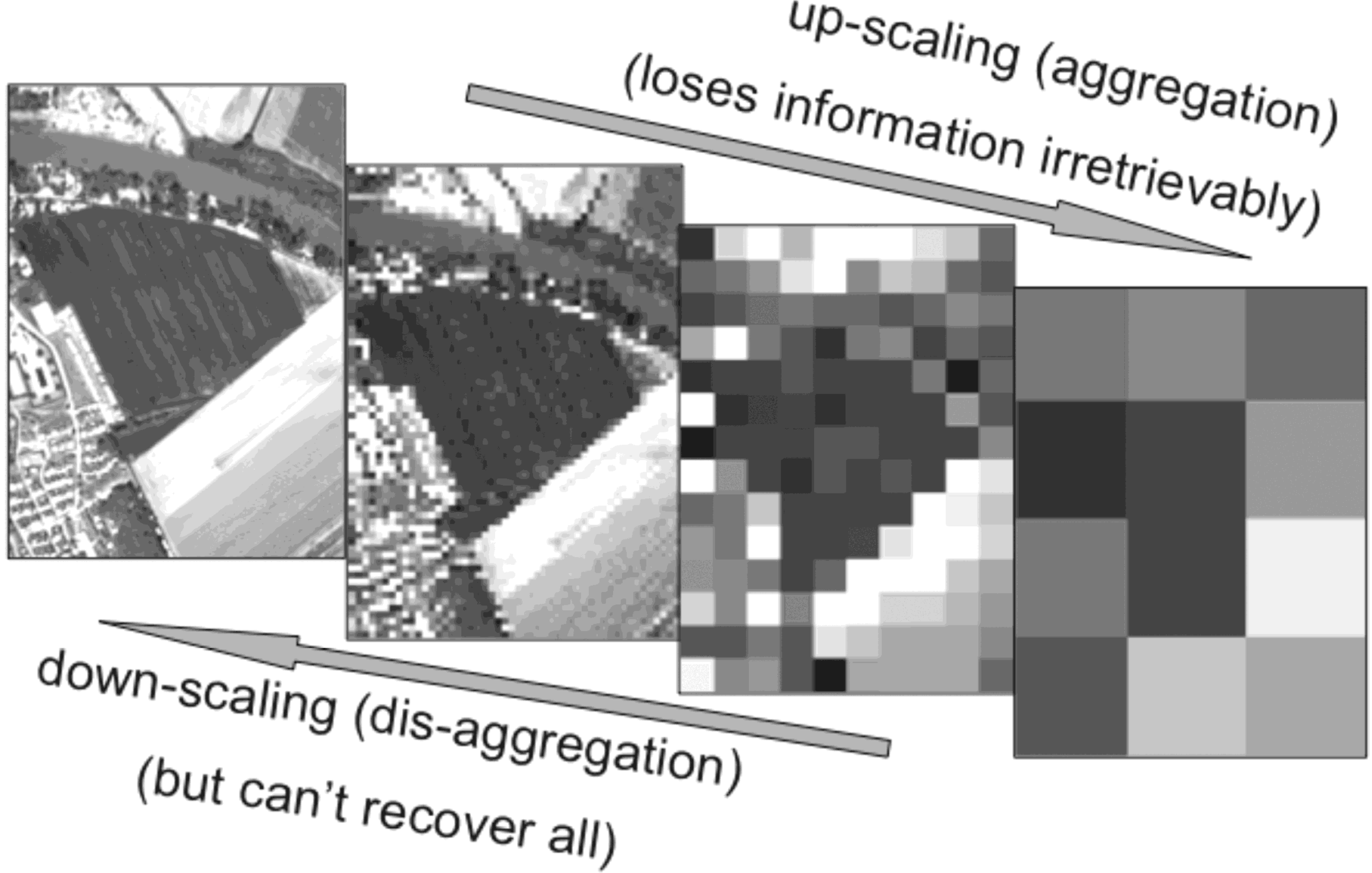
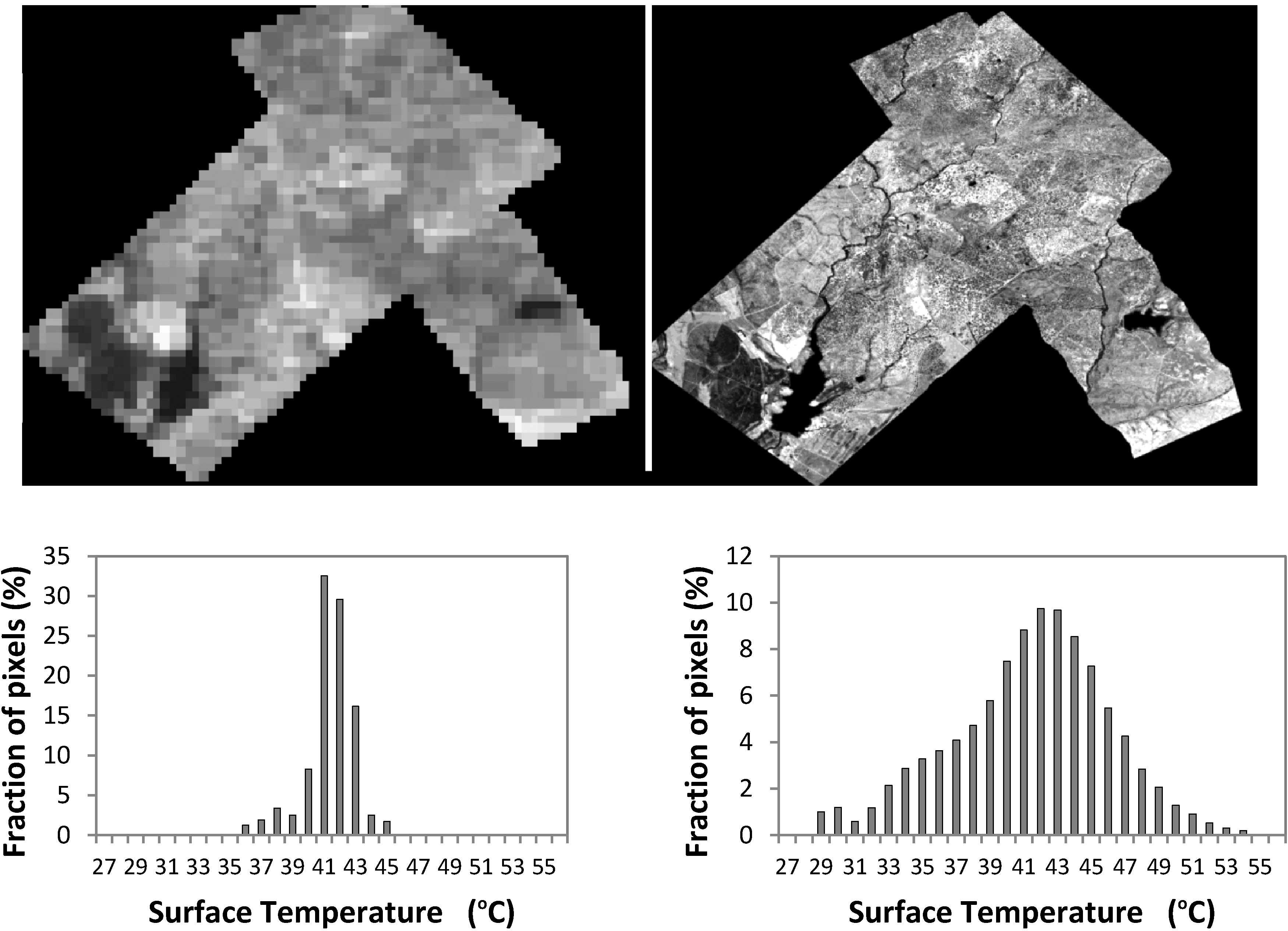
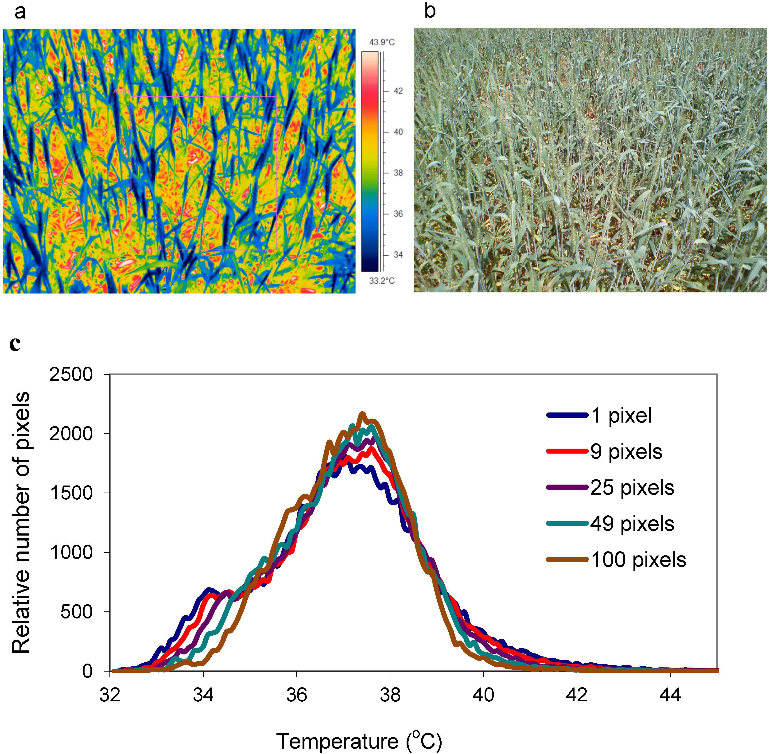
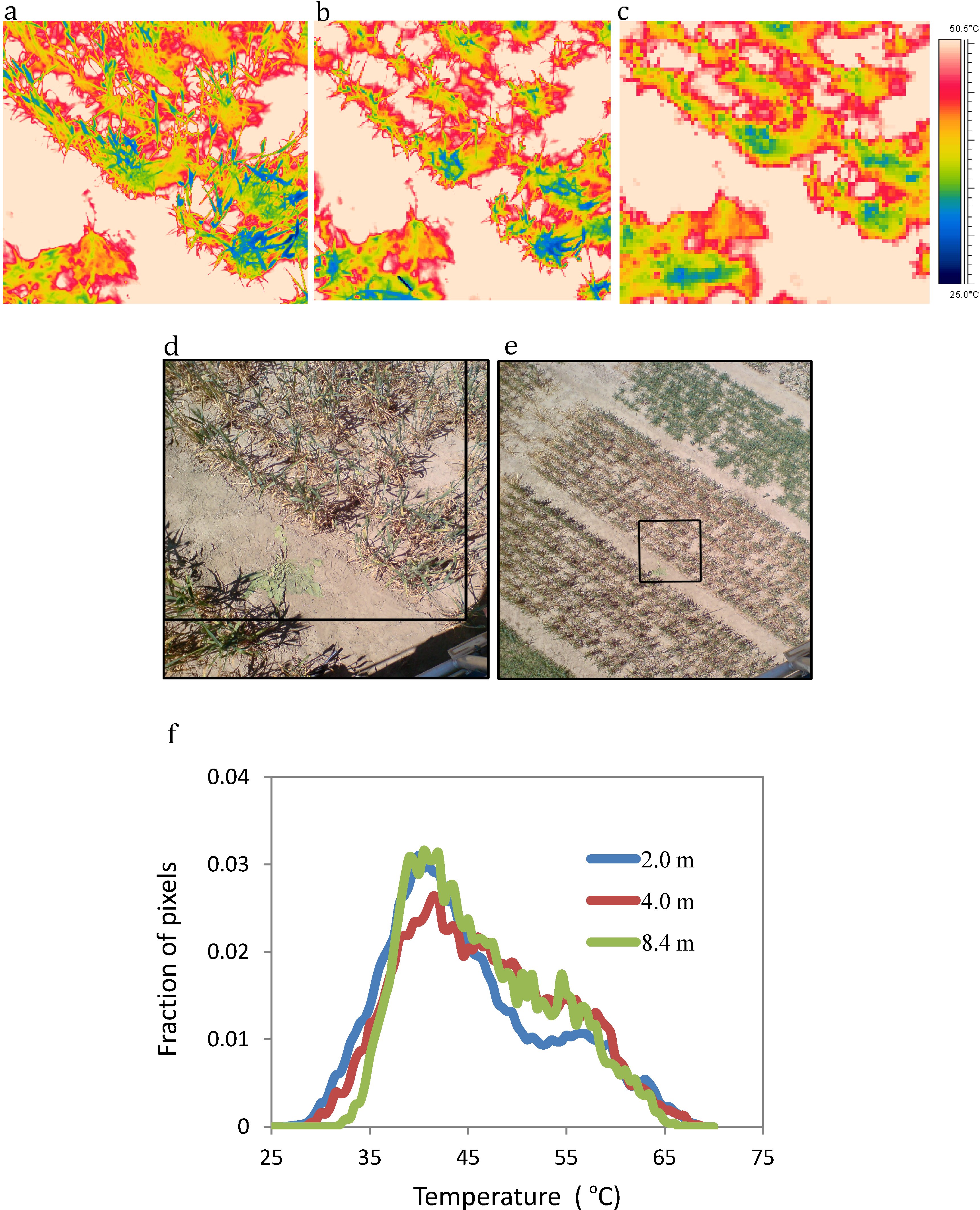
2. Impacts of Image Scale on Thermal Imaging for Plant Phenotyping

The most obvious effect of the aggregation of thermal images (or of reductions in spatial resolution) is that the frequency distribution of observed temperatures becomes narrower with truncation of the extremes and reduction or elimination of intermediary peaks. Some examples of the changing frequency distributions with thermal images obtained at different spatial resolutions are shown in Figure 2 and Figure 3 while the effect of artificial pixel aggregation is shown in Figure 4.
Figure 2. Thermal images from (a) a satellite (Landsat 5 at 120 m spatial resolution) and (b) airborne sensors (DAIS at 3 m spatial resolution) taken over an area of Montado rangeland near Evora, Portugal (June 2006), with corresponding temperature histograms (c) and (d) showing the increase in temperature range with smaller pixels.
Agronomy 04 00380 g002
Figure 3. Thermal images of a given sparse area of a wheat crop obtained from a “cherry-picker” (November 26, 2009; taken with a FLIR SC660 (640 × 480 pixels) imager with a 19 mm lens) from (a) 2.0 m; (b) 4.0 m; and (c) 8.4 m, together with corresponding RGB images from 2.0 m (d) and 8.4 m (e). The pixel sizes increase from (a) to (c) with the corresponding temperature frequency histograms (f) becoming narrower.
Agronomy 04 00380 g003
Figure 4. Illustration of the consequences of pixel binning (aggregation) for a thermal image for a wheat crop (approximately 73% green leaf area in the image). (a) Thermal image taken with a FLIR SC660 camera; (b) corresponding RGB image; and (c) and the temperature frequency histograms for binning of 2 × 2, 3 × 3, 4 × 4 . . . 10 × 10 pixels, showing that the small peak (indicated by an arrow) representing the cool ears is only apparent for the highest spatial resolution images.
Agronomy 04 00380 g004
The observed temperature distribution is important for the analysis of thermal images: Not only does it allow one to separate temperatures of different components of the image, but each type of object will have a range of temperatures depending on local conditions such as exposure to sunlight. The narrowing of the temperature distribution with coarser spatial resolution or increased pixel aggregation can lead to large changes in the extreme temperatures observed: for example, the minimum temperature detected in the area shown in Figure 3 rises from 29.0 °C in (a), through 31.7 °C in (b) to 34.4 °C in (c) as the sensor distance increased from 2 to 8.4 m. This has clear implications for estimates of canopy temperature where there are mixed pixels.
Indeed, it has been suggested that canopy temperature can be extracted automatically from an image containing pixels representing both canopy and background, each having their own characteristic temperatures, either by eliminating all pixels outside the expected temperature range for the leaves [7], or by the use of automated thresholding algorithms such as the Otsu method (e.g., [8]). The image in Figure 4 appears to be a good example where such an approach should work effectively, as the flowering shoots stand out very clearly as colder than the background in the thermal image. Inspection of the temperature frequency distribution (Figure 4c) shows that for the unaggregated data it is clearly bimodal with a small peak that apparently represents the flowering shoots and a broader peak that appears to be dominated by temperature background. As shown in Figure 5, the overall histogram can be assumed to be the sum of two separate Gaussian curves representing the two main components of the image. Although the thresholding algorithm works well on the highest resolution version of the image (where the pixel size similar to that of individual leaves), as soon as pixel aggregation is performed to reduce the spatial resolution, not only does the mean position of the minor peak change, but it also rapidly disappears (Figure 4c) as an increasing proportion of pixels become mixed.
Figure 5. Illustration of the contribution of leaf and background soil temperatures to the overall temperature histogram (data from the highest resolution image in Figure 4, extracted using the Otsu thresholding method [8]).
Agronomy 04 00380 g005
The absolute temperature and its frequency distribution are also important in calculations of evaporation or transpiration rates. Although any temperature biases are not critical in phenotyping applications, biased data can lead to significant errors when substituted into the energy balance Equation [8] to estimate stomatal conductance or transpiration. Accurate calculations require that true estimates are available for the leaf temperatures of different surfaces such as shaded and sunlit leaves. This variability of leaf temperature (and the corresponding variability of wet or dry reference leaf temperatures) can affect the precision of estimates of canopy stomatal conductance or evaporation [9,10].

3. Review and Evaluation of Methods for Extraction of Component Temperatures

Approaches to the extraction of sub-pixel information can be conveniently classified into (i) those that operate at the whole pixel level; and (ii) those that work at the sub-pixel level. Although these two approaches can overlap, we will consider them separately in what follows. More detail may be found in remote sensing texts such as [5,11,12] and in appropriate reviews [13].

3.1. Whole Pixel Approaches to Extraction of True Leaf Temperatures

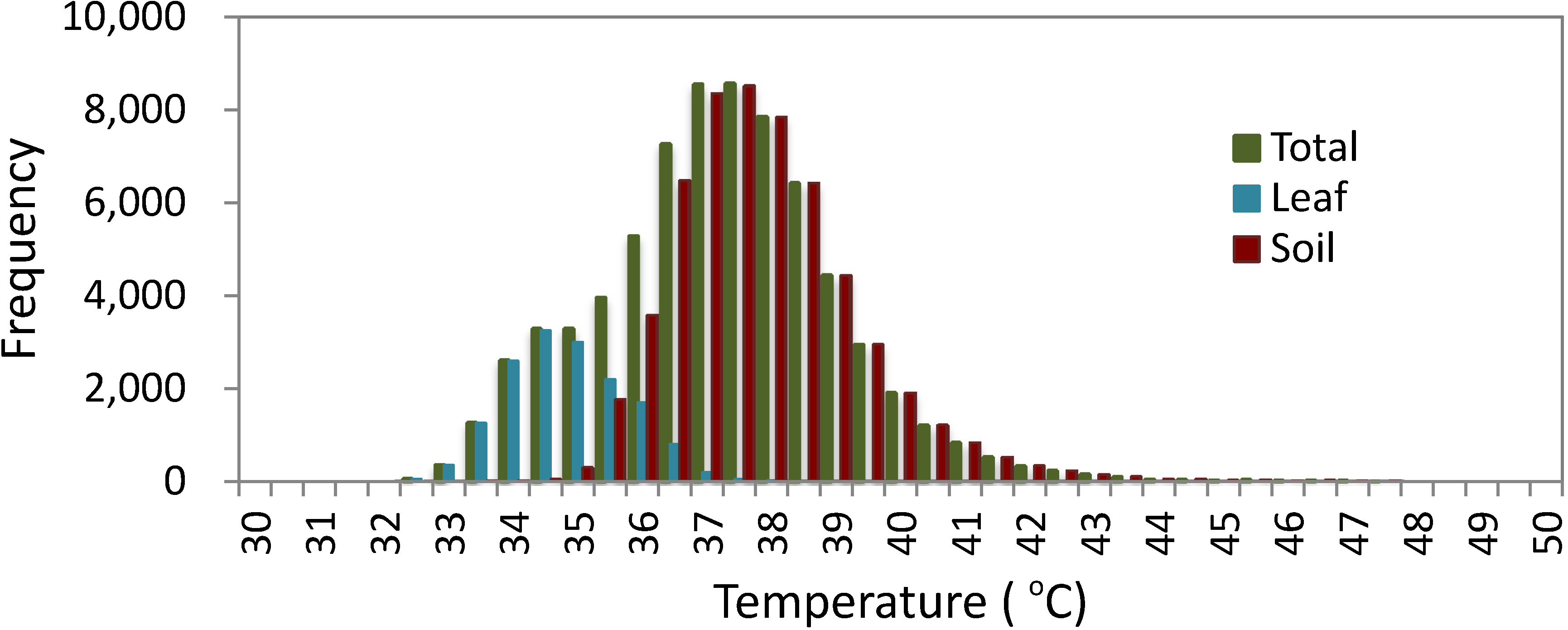
3.1.1. Histogram Analysis

The most straightforward approach to the extraction of temperatures of canopy components such as sunlit leaves is to identify pixels that correspond to canopy or background based on an analysis of the distribution of temperatures among the population of pixels and to use this to segment the image into two (or more) classes. Where there is a clear difference between the average temperature of the canopy elements and of the background, as for example when the soil is much hotter than the evaporating canopy, the histogram of frequency against temperature will be bimodal and it becomes straightforward to derive thresholds delimiting the two classes of pixel and hence segmenting the image into (predominantly) leaf and (predominantly) background classes. Omitting pixels from near the threshold as most likely to represent mixed pixels allows one to obtain useful estimates of the canopy temperature from the remaining pixels.
Heuristic visual identification of the separate peaks can be effective where they exist, while a range of automated algorithms are available that can also operate where clear peaks are not apparent. A wide range of such automated algorithms are available for thresholding and are implemented in imaging software such as Fiji [14]; methods available include isodata [15], Otsu thresholding [8], and various types of entropy-based thresholding [16,17]. Where the histogram does not show two clear peaks, however, such methods can fail.
Examples of the use of threshold analysis for the isolation of pixels relating to leaf temperatures include the early use of a background sheet [7] and the more recent use of thresholding in a controlled environment cabinet for selection of pixels relating to leaves [18]. Unfortunately, this approach is critically dependent on the scale of the image used as is illustrated in by the results in Figure 3 and Figure 4. Although one might think that use of the minimum temperature (as an indicator of the plant temperature) might be a useful alternative to thresholding—as this will largely eliminate the problem of mixed leaf/background pixels—the marked dependence of the minimum (e.g., Figure 3) on scale means that absolute temperatures cannot readily be obtained by this means. Of course, the minimum value may be somewhat subject to error (representing only one pixel) so it may be better to take some (arbitrary) lower percentile of the data [19].

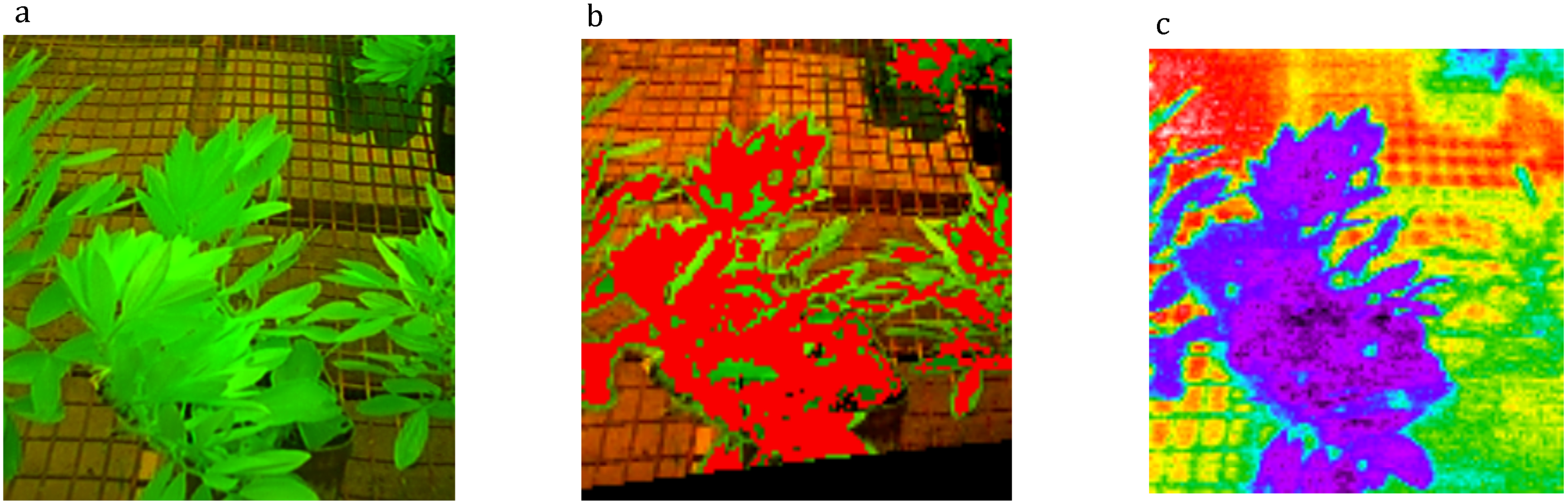
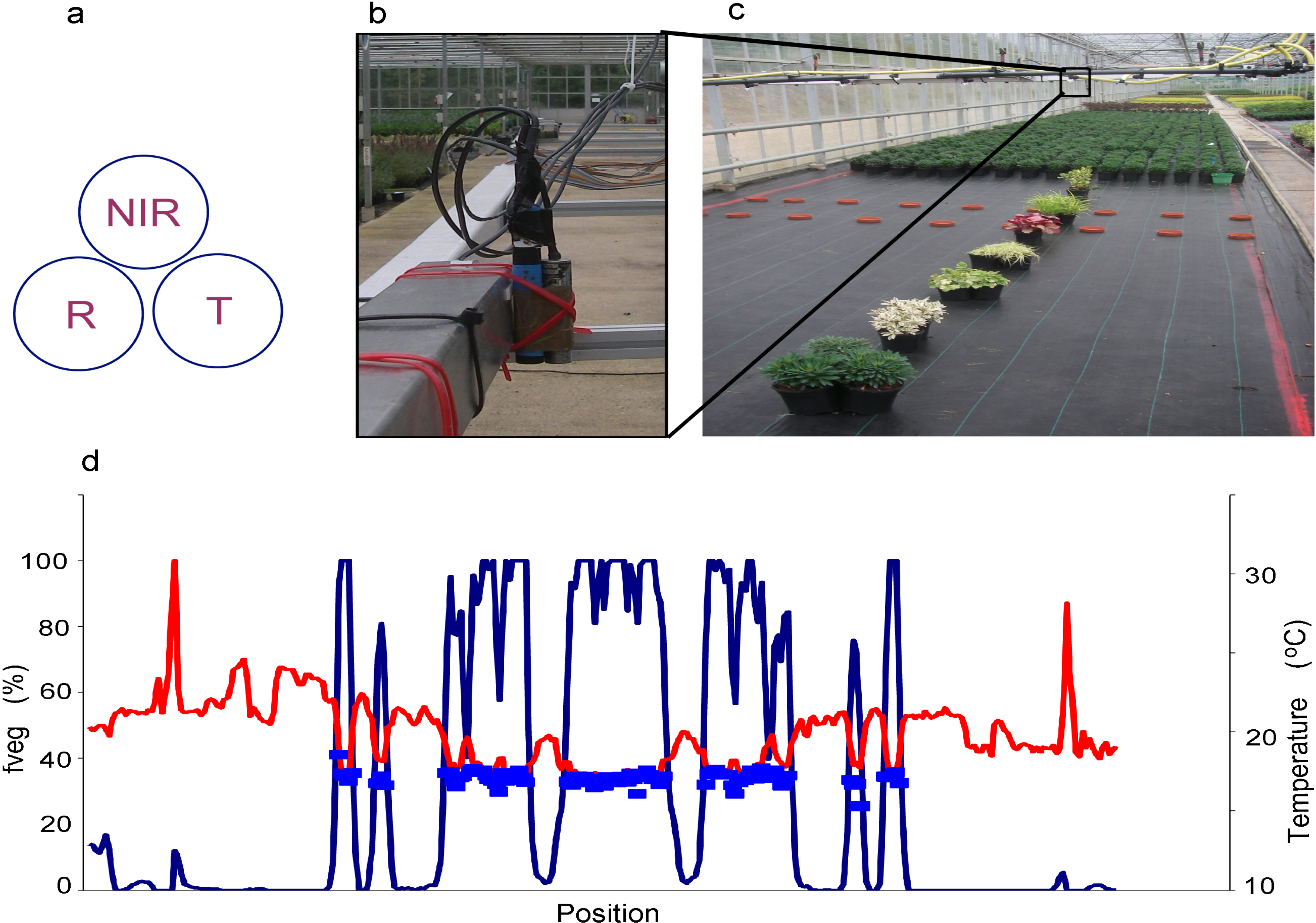
3.1.2. Image Segmentation by Cross-Correlation with a Spectral Image
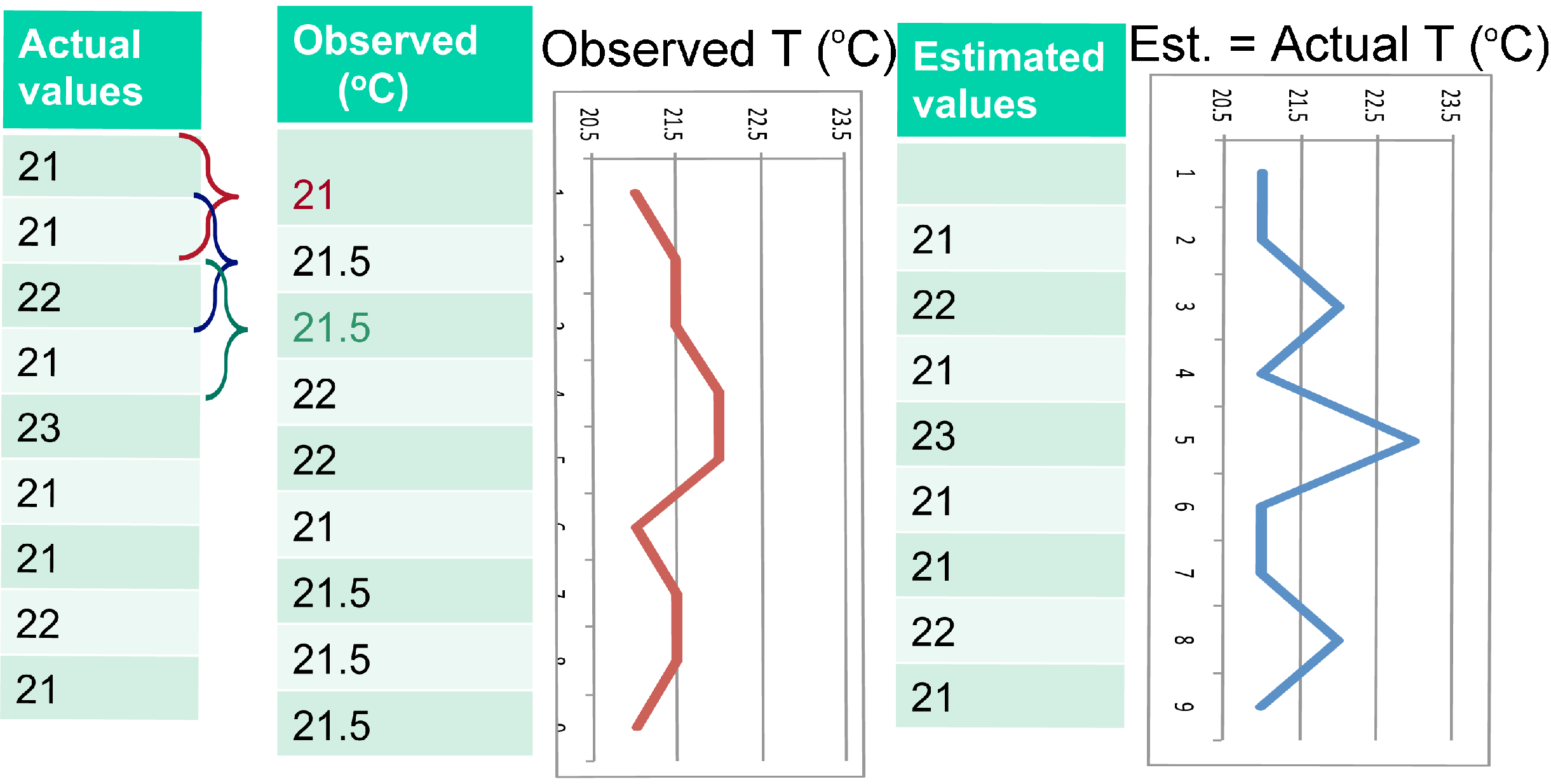
An alternative approach to the use of whole pixels involves the use of additional information, such as that derived from a simultaneous overlaid RGB, multispectral or hyperspectral image, to identify relevant “plant” pixels (Figure 6). The ancillary image is used to identify pixels representing plant and to separate them from pixels representing background, often on the basis of vegetation indices (VI) based on the difference between reflectance in the red (R) and near infrared (NIR), such as the Normalised Difference Vegetation Index (NDVI), though standard image-processing tools such as the magic wand in software such as Adobe Photoshop (Adobe, San Jose, CA, USA) can work well for identifying leaves in RGB images.
Figure 6. An example of automated image processing to determine the temperature of plant leaves in an image where only part of the image is relevant. (a) Shows an original visible image, while (b) shows the result of image classification of the original image, using the ENVI spectral angle mapper algorithm, showing areas classified as leaf in red (presented after warping and resampling to match the thermal image). (c) Thermal image corresponding to the classified image so that leaf temperatures can then be extracted for the pixels in the thermal image that correspond to the red areas in (b). Based on data from Leinonen and Jones [20].
Agronomy 04 00380 g006
Details on the derivation of different vegetation indices and their application can be found in many remote sensing texts (e.g., [5,11,21,22]) while a discussion of pitfalls in their use may be found in [5]. The use of vegetation indices is routine in satellite remote sensing and has also been widely used in crop-scale studies to identify canopy within the image [20,23,24,25]. In this approach, one uses the ancillary image to identify areas of complete vegetation cover (omitting mixed or non-canopy pixels) to determine the true temperature of leaves without any bias that would result from inclusion of background. The approach requires that the thermal and the ancillary image are accurately co-registered; in practice this is often difficult at a single pixel level, as a result of slight differences in view angle resulting from parallax errors or as a result of leaf movement when images are not exactly synchronised. Co-registration of information can be facilitated by including physical markers that are clearly identifiable across image modalities and/or by using algorithms based on feature correspondences (e.g., scale invariant feature transform or SIFT aims at detecting and describing local features in images which can then be matched across modalities). It is worth noting that parallax errors can be reduced by aggregation of pixels into larger areas, though with the usual loss of information associated with aggregation. In addition to providing an estimate of presence/absence of vegetation in any pixel, it is possible to use calculated VI to estimate a fraction of vegetation cover in the pixel (fveg); this will be discussed in the next section.
An extreme example of such an up-scaling approach is to combine the field of an infrared thermometer with supplementary information from narrow angle red and near infrared radiometers that sample reflectance from a similar area to provide an associated estimate of an appropriate VI (see Figure 7 below).

3.1.3. Mixed Pixels

Rather than just attempting to identify pure pixels, the approach can be extended to use of the ancillary information to quantify the proportion of any pixel that is occupied by vegetation and hence to estimate the temperature of the vegetation component. This type of approach has been widely applied to satellite imagery for estimation of crop stress indices from thermal channels for irrigation scheduling purposes, where the large pixels acquired from MODIS or even Landsat inevitably contain both canopy and background soil. This method is particularly suited to the analysis of IR images acquired at height (e.g., from blimp or UAV) where relative comparison of canopy temperature of a large number of genotypes spread over a wide area is considered. There are again several approaches available to estimate the vegetation fraction in the pixel of which perhaps the most powerful is based on spectral unmixing (see [5,6,11]). Given spectra for the pure end members, it is possible to estimate the fraction of each pixel which is vegetation (fveg) using any standard image processing software such as Matlab (Mathworks, Natick, MA, USA), ERDAS Imagine (Hexagon Geospatial, Stockholm, Sweden), or ENVI (Exelis Visual Information Solutions Inc., Boulder, CO, USA).
A simpler approach that is applicable to estimation of fveg is to use the scaled vegetation index (VI*) where:
fveg ≈ VI* = (VI − VImin)/(VImax − VImin)
where VImin and VImax are the minimum (pure soil) and maximum (pure vegetation) vegetation indices and it is assumed that the VI is linearly related to fveg. Although NDVI is commonly used as the vegetation index in this formulation, unfortunately NDVI is frequently non-linearly related to fveg (see [5]) so it is generally better to use the simple difference vegetation index (= NIR-R) which is more linearly related to fveg in this formula. Others have used simple regression between observed vegetation indices and canopy cover to estimate fveg [26]. Assuming that temperatures combine linearly [5] one can write:
Tpixel = Tveg × fveg + Tsoil (1 − fveg)
where Tpixel, Tsoil and Tveg, respectively, are the pixel average, soil and vegetation temperatures. It follows that one can derive the temperature of the canopy component as long as one has Tpixel, Tsoil (which may be obtained for an area of pure soil) and fveg. This is the basis for a significant number of published approaches to the estimation of canopy temperature for the calculation of crop water stress indices (see for example [5,27]). Related approaches include the “triangle” or “trapezoid” methods used for estimation of either surface water content [27,28] or a crop water stress index (a measure of stomatal opening) [29] from satellite data. A critical limitation of triangle (or trapezoid) methods using satellite data is that they generally depend on estimation of the vertices from the extreme pixels on a plot of temperature against VI, but in most images pure extremes may not exist (especially the non-transpiring pure vegetation point) [5].
An alternative approach that avoids a need for explicit estimates of Tsoil that is suitable for satellite images with large numbers of pixels at different temperatures and canopy covers [26] is to estimate the canopy temperature from covariance analysis of fveg and T and extrapolation to 100% canopy cover. Another approach that avoids the need for an explicit estimate of Tsoil is to extract estimates of both soil and vegetation temperatures from the use of multiangular images [30,31]. Clearly the number of temperatures that can be extracted depends on the number of independent view angles, with the two angles obtained with ATSR-2 radiometer on the ERS satellite being adequate to derive soil and vegetation temperatures by simultaneous solution of equation (2) when one has obtained the apparent fveg at each view angle from the multispectral data [30]. One can also use a canopy radiation transfer model to constrain the temperature extraction as has been proposed by Timmermans et al. [31] for the extraction of sunlit and shaded soil and leaf temperatures.
Figure 7. (a) Plan view, and (b) and (c) photographs, of triplet sensor (containing three narrow field of view (6°) sensors, one NIR (800 nm), one R (660 nm) and an infrared thermometer (Calex 101A) to estimate temperature of different plants with differing chlorophyll contents; (d) Output of sensor during transect of the pots shown in (c), where the red line represents measured temperature at any point, the blue line represents the fveg (expressed here as a percentage) calculated from the R and NIR sensors, and the blue squares represent calculated temperatures for any reading where fveg > 50%.
Agronomy 04 00380 g007
An interesting alternative approach [32] has been proposed that makes use of the differing temperature response in the short-wave thermal infrared (3.55–3.93 μm) and long-wave thermal infrared (10.5–11.5 μm) bands of the AVHRR sensor on the NOAH-6 satellite. Because the radiation emitted in the short-wave thermal band increases much more rapidly with increasing temperature than does that in the long-wave band, these authors showed that it was possible to identify sub-pixel high temperature sources from satellite images and to estimate both their temperature and the size of the source. Unfortunately, this approach is not in general applicable to crop phenotyping as it requires measurements to be made at night (because the short-wave thermal bands is subject to interference by solar radiation during the day) and because the temperature differences between crop and background tend to be small (less than 20 K) as compared with the situation discussed by Matson and Dozier where temperature differences were more than 175 K [32].

3.2. Spatially Precise Sub-Pixel Approaches (Dis-Aggregation)
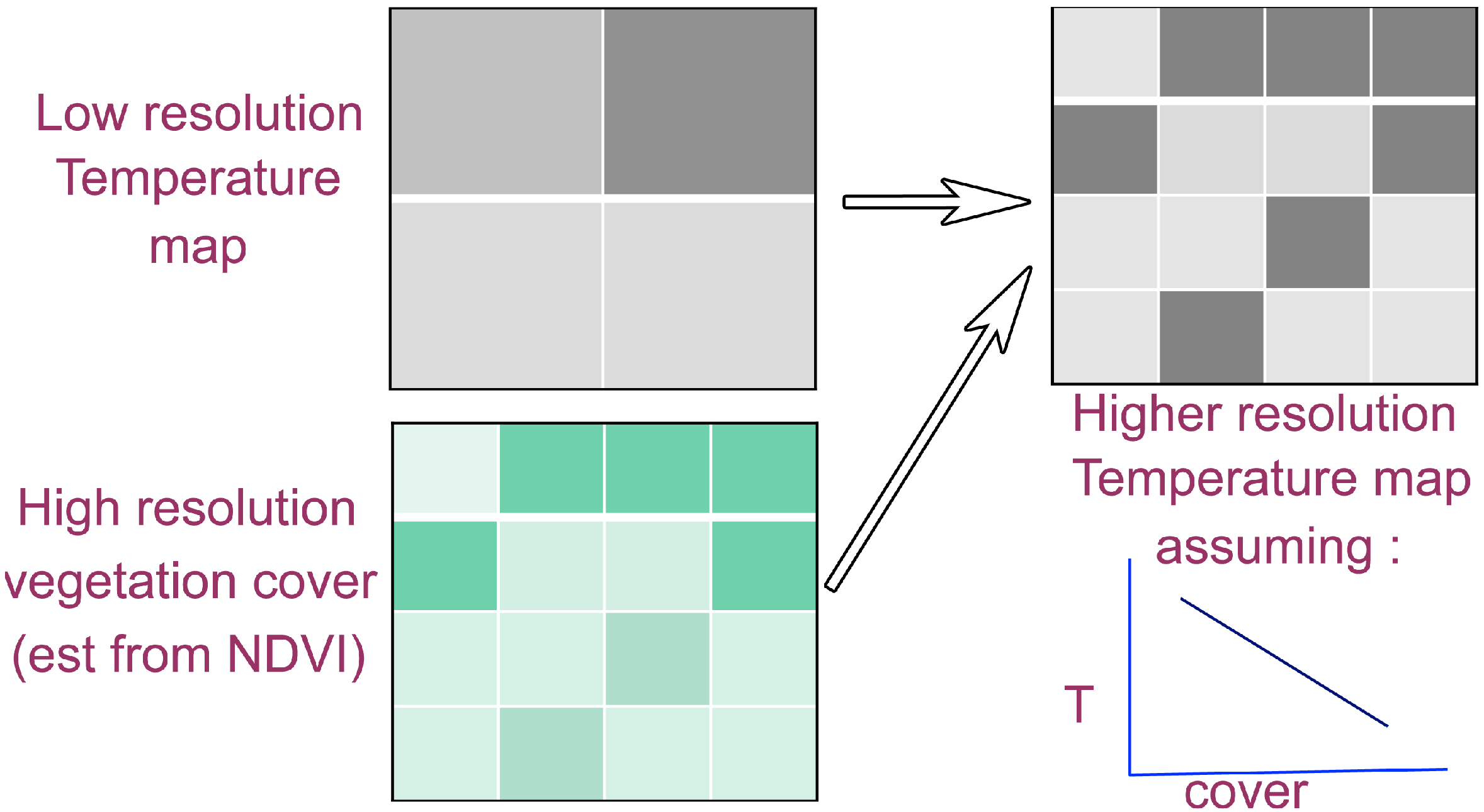
As we have seen, in most cases, both when using thermal imagery and when using spot thermal sensors, the ifov often covers a heterogeneous area that is not pure leaf. Methods for extraction of the component temperatures, but without any sub-pixel spatial information, have been outlined above. It can also be possible to derive spatial information at a sub-pixel scale if we have appropriate additional spatial information. The two main possibilities are (a) data fusion and (b) oversampling.

3.2.1. Data Fusion

This widely used approach involves combining a lower spatial resolution thermal image with finer spatial resolution data, such as from a multi- or hyperspectral image (for further details see any remote sensing text, e.g., [5,11]). The general method is illustrated in Figure 8 where temperature in thermal pixels over an appropriate area is regressed against the corresponding aggregated average fveg from the corresponding high resolution pixels. The temperature for each high resolution sub-pixel is then estimated (Figure 8—top right) from this regression line (Figure 8—bottom right) using the appropriate fveg for that sub-pixel. This approach was developed by Kustas and colleagues [33] and has been successfully applied to the disaggregation of low spatial resolution (approximately 5 km) GOES satellite thermal data by the use of high spatial resolution NDVI data obtained from aircraft. A key requirement for this approach is an ability to overlay accurately the thermal and spectral images; although readily achieved at the satellite scale, this process can be imprecise where there is a parallax error as when different images are taken from different positions, as is common in field phenotyping situations where images frequently need to be obtained at close range (1–2 m) with thermal cameras where the visible image is offset from the thermal by perhaps 5 cm.
Figure 8. An illustration of the process of image fusion for the derivation of a higher resolution temperature map (top right) from a low resolution map and a high resolution vegetation cover map, by the use of an assumption regarding the relation between vegetation cover and temperature (as shown in the bottom right image).
Agronomy 04 00380 g008

3.2.2. Oversampling (or Image Deconvolution)

A technique, variously called oversampling, blind deconvolution or super-resolution imaging, originally developed for astronomical studies, potentially allows one to increase the effective spatial resolution from sub-pixel movements of the sensor (see e.g., [34,35,36]). In its simplest form, the approach is based on the oversampling algorithm where, for example for the case of sub-pixels half the linear dimensions of the full observed pixel, the calculated value (Vn) the nth sub-pixel in a linear vector is given by:
Vn = On × 2 − Vn-1 = On × 2 − (On-1 × 2 − (On-2 × 2 − ( . . . . . (On-i × 2 − I)))
where On is the nth observation, and On-i is the observation on the initial pixel set as equal to a known initial value, I (this initial value is chosen for an area of constant temperature larger than a single pixel). To generate the values for all four sub-pixels in a square pixel it is necessary to run a similar formula for both the x and y directions. This procedure is illustrated schematically in Figure 9.
Figure 9. Illustration of the oversampling process in one dimension. The original high resolution data set is shown on the left, with the observations calculated as the average of two adjacent values in the second column, while the estimated (calculated) values (which equal the original) are shown in the third column.
Agronomy 04 00380 g009
Although in principle such an approach can reconstitute exactly the underlying high resolution vector from the overlapping lower resolution vector with each value displaced by half a pixel, this does not usually work in practice because noise (error both in the values observed and in their spatial placement) leads to potential instability in the algorithm. Successful practical application therefore requires an optimisation routine (e.g., based on iterative data fitting) to get the best-fitting enhanced results; this can be achieved through the use of any one of several image deconvolution algorithms [34,36].

4. Technical Aspects Relating to Choice of Sensor

From a practical point of view, determining which infrared sensor to use for phenotyping plants in the field, glasshouses or in the lab depends largely on the application: are relative temperature estimates sufficient for one’s purpose or does one need absolute temperature measurements? Is the sensor to be mounted on a moving platform (UAV, blimp, Phenomobile) or on a fixed one (cherry picker, tripod). There is no general consensus that establishes which sensor is the best for a given application. However, the following factors should be considered to save both time and money:

4.1. Realistically Define the Objective of the Experiment and Define an Instrument Specification that Meets These Minimum Requirements

The specifications should at least define the precision (“repeatability”), accuracy and sensitivity of the thermal sensor required. Note that requirements for higher accuracy and higher thermal sensitivity (better than 0.05 K) will increase drastically the price of the sensor. High absolute accuracy may not be needed where relative measurements only are needed (see [37] for discussion of this point).

4.2. Determine the Required Speed of Response of the Sensor

The mode of operation of a phenotyping platform (moving or fixed) will determine the frequency at which data needs to be collected. If the platform is required to move fast in order to limit the effects of environmental variation, a higher frequency of data acquisition would be necessary. Higher rates will ensure that data points are available for all experimental units. For example, if one aims at measuring the temperature of a 10 mm-wide leaf with a thermopile sensor travelling at 1 m s−1, a sensor measuring at >100 Hz would be required to capture a non-mixed temperature data point. The drawback of increasing frequency is a substantial cost increase for the sensor.

4.3. Establish the Spatial Resolution of the Sensor (and Its Optics)

It is necessary to determine the smallest object of interest. Higher resolution infrared cameras can measure smaller targets from farther away, but their price increases non-linearly as a function of the micro-bolometer size. The field of view of the sensor is determined by the optics—a wider field of view will tend to increase the problem of mixed pixels. Today, IR cameras with megapixel resolution are available on the market but their price is in excess of k$150.

5. Conclusions

This review has briefly outlined the main ways in which image scale is important for the use of thermal imaging of plant leaves and canopies in the field for phenotyping purposes. High spatial resolution (with pixels substantially smaller than the objects of interest) is usually necessary to obtain accurate estimates of the object temperature without confounding by mixed pixels. Where spatial resolution is larger than the size of the objects (e.g., leaves when imaging canopies), it is necessary to allow for the errors introduced if we are to get accurate estimates of temperature for use in calculation of stomatal conductance or transpiration. For simple phenotyping applications, however, where one is simply comparing genotypes, the absolute temperatures tend to be of limited interest and consistent biases (e.g., as introduced by using extreme values at a constant scale) may not be a problem. Any recommendations as to the spatial scale at which one should observe a plant/canopy depends on the hypotheses being tested and the need to derive relative or absolute temperature, and whether or not one needs to overlay images from different sensors; no simple generalisation can be made. Nevertheless, smaller pixels always give more information, including for example even information about temperature variability (which itself may be a useful diagnostic of stress [38]), something that is not available where individual pixels cover several leaves or whole canopies. There will, however, always be a trade-off between information collected and the speed of data acquisition (sometimes determined by processing power and the need for subsequent image processing or even data storage capacity). Sometimes excessive detail provided by smaller pixels can hide the general picture, while smaller pixels also make it more difficult to overlay images from different sensors. Where leaf-scale information is required, there will be a general need for pixels to be smaller than the leaves which may be 0.5 cm or less for small grain cereals, but as large as 10 cm or more for larger leaved crops such as maize or grapevine. We stress that careful consideration of the image acquisition method (e.g., images acquired under specific environmental conditions, variation in IR sensor angle in relation to plant/canopy structure) is invaluable to make the analysis of IR images more straightforward and limit issues associated with mixed pixels.
Notwithstanding the importance of image scale in the use of thermal imaging, it should not be forgotten that many other factors affect the accuracy and utility of such approaches. These include factors such as canopy height (affecting boundary layer energy transfer processes), canopy structure and illumination (affecting leaf illumination) and even time of day, which can affect the magnitude of genetic variation in stomatal conductance [1,3]. To this date, a complete treatise of the influence of canopy architecture on remote sensing of canopy temperature has not been forthcoming. This is in part due to the complexity in quantifying plant architecture and temperature, simultaneously. However, the use of 3D digitisation technologies (which explicitly describe the 3D geometry and topology of plants) associated with IR imaging (e.g., [39]) are starting to provide some new insights that ultimately will close this knowledge gap.
The various considerations discussed here will need to be incorporated into any phenotyping or precision agriculture application of thermal imaging. Perhaps, the difficulties involved interpreting thermal imagery, together with the technical problems of associating temperatures with specific plots, are the underlying reasons why publications on published applications of thermography to crop phenotyping are still very few [3,4,40,41]. The scaling problems have only been addressed substantially in the application of satellite imagery for irrigation scheduling with the use primarily of NDVI to estimate actual canopy surface temperature [5].

Acknowledgments

This work was made possible by internal funding sources from CSIRO—Phenomics Informatics and Modelling Tools, the High Resolution Plant Phenomics Centre under the Australian government National Collaborative Research Infrastructure Strategy (Australian Plant Phenomics Facility) and the HRPPC’s innovators in-residence program.

Author Contributions

Each author contributed equally to this paper.

Conflicts of Interest

The authors declare no conflict of interest.

References

  1. Jones, H.G. Application of thermal imaging and infrared sensing in plant physiology and ecophysiology. Adv. Bot. Res. 2004, 41, 107–163. [Google Scholar] [CrossRef]
  2. Saint Pierre, C.; Crossa, J.; Manes, Y.; Reynolds, M.P. Gene action of canopy temperature in bread wheat under diverse environments. Theor. Appl. Genet. 2010, 120, 1107–1117. [Google Scholar] [CrossRef]
  3. Jones, H.G.; Serraj, R.; Loveys, B.R.; Xiong, L.; Wheaton, A.; Price, A.H. Thermal infrared imaging of crop canopies for the remote diagnosis and quantification of plant responses to water stress in the field. Funct. Plant Biol. 2009, 36, 978–989. [Google Scholar] [CrossRef]
  4. Romano, G.; Zia, S.; Spreer, W.; Sanchez, C.; Cairns, J.; Araus, J.L.; Müller, J. Use of thermography for high throughput phenotyping of tropical maize adaptation in water stress. Comput. Electron. Agric. 2011, 79, 67–74. [Google Scholar] [CrossRef]
  5. Jones, H.G.; Vaughan, R.A. Remote Sensing of Vegetation: Principles, Techniques, and Applications; Oxford University Press: Oxford, UK, 2010; p. 369. [Google Scholar]
  6. Shi, C.; Wang, L. Incorporating spatial information in spectral unmixing: A review. Remote Sens. Environ. 2014, 149, 70–87. [Google Scholar] [CrossRef]
  7. Giuliani, R.; Flore, J.A. Potential use of infra-red thermometry for the detection of water stress in apple trees. Acta Hortic. 2000, 537, 383–392. [Google Scholar]
  8. Otsu, N. A threshold selection method from gray level histograms. IEEE Trans. Syst. Man Cybern. 1979, 9, 62–66. [Google Scholar] [CrossRef]
  9. Guilioni, L.; Jones, H.G.; Leinonen, I.; Lhomme, J.P. On the relationships between stomatal resistance and leaf temperatures in thermography. Agric. For. Meteorol. 2008, 148, 1908–1912. [Google Scholar] [CrossRef]
  10. Leinonen, I.; Grant, O.M.; Tagliavia, C.P.P.; Chaves, M.M.; Jones, H.G. Estimating stomatal conductance with thermal imagery. Plant Cell Environ. 2006, 29, 1508–1518. [Google Scholar] [CrossRef]
  11. Jensen, J.R. Remote Sensing of the Environment: An Earth Resource Perspective, 2nd ed.; Pearson Prentice Hall: Upper Saddle River, NJ, USA, 2007; p. 592. [Google Scholar]
  12. Lillesand, T.M.; Kiefer, R.W.; Chipman, J.C. Remote Sensing and Image Interpretation, 6th ed.; John Wiley & Sons: New York, NY, USA, 2007; p. 768. [Google Scholar]
  13. Atkinson, P.M. Downscaling in remote sensing. Int. J. Appl. Earth Observ. Geoinf. 2013, 22, 106–114. [Google Scholar] [CrossRef]
  14. Fiji Is Just ImageJ. Available online: http://fiji.sc/wiki/index.php/Fiji (accessed on 2 July 2014).
  15. Ridler, T.W.; Calvard, S. Picture thresholding using an iterative selection method. IEEE Trans. Syst. Man Cybern. 1978, 8, 630–632. [Google Scholar] [CrossRef]
  16. Kapur, J.N.; Sahoo, P.K.; Wong, A.C.K. A new method for gray-level picture thresholding using the entropy of the histogram. Graph. Model. Image Process. 1985, 29, 273–285. [Google Scholar]
  17. Li, C.H.; Tam, P.K.S. An iterative algorithm for minimum cross entropy thresholding. Pattern Recognit. Lett. 1998, 188, 771–776. [Google Scholar]
  18. Sirault, X.R.R.; James, R.A.; Furbank, R.T. A new screening method for osmotic component of salinity tolerance in cereals using infrared thermography. Funct. Plant Biol. 2009, 36. [Google Scholar] [CrossRef]
  19. Jones, H.G.; Stoll, M.; Santos, T.; de Sousa, C.; Chaves, M.M.; Grant, O.M. Use of infrared thermography for monitoring stomatal closure in the field: Application to grapevine. J. Exp. Bot. 2002, 53, 2249–2260. [Google Scholar] [CrossRef]
  20. Leinonen, I.; Jones, H.G. Combining thermal and visible imagery for estimating canopy temperature and identifying plant stress. J. Exp. Bot. 2004, 55, 1423–1431. [Google Scholar] [CrossRef]
  21. Sabins, F.F. Remote Sensing—Principles and Interpretation; W. H. Freeman and Company: New York, NY, USA, 1997; p. 494. [Google Scholar]
  22. Rees, W.G. Physical Principles of Remote Sensing, 2nd ed.; Cambridge University Press: Cambridge, UK, 2001; p. 343. [Google Scholar]
  23. Möller, M.; Alchanatis, V.; Cohen, Y.; Meron, M.; Tsipris, J.; Naor, A.; Ostrovsky, V.; Sprintsin, M.; Cohen, S. Use of thermal and visible imagery for estimating crop water status of irrigated grapevine. J. Exp. Bot. 2007, 58, 827–838. [Google Scholar]
  24. Chaerle, L.; Leinonen, I.; Jones, H.G.; Van Der Straeten, D. Monitoring and screening plant populations with combined thermal and chlorophyll fluorescence imaging. J. Exp. Bot. 2007, 58, 773–784. [Google Scholar]
  25. Berni, J.A.J.; Zarco-Tejada, P.J.; Sepulcre-Cantó, G.; Fereres, E.; Villalobos, F. Mapping canopy conductance and cwsi in olive orchards using high resolution thermal remote sensing imagery. Remote Sens. Environ. 2009, 113, 2380–2388. [Google Scholar] [CrossRef]
  26. DeTar, W.R.; Penner, J.V. Airborne remote sensing used to estimate percent canopy cover and to extract canopy temperature from scene temperature in cotton. Trans. Am. Soc. Agric. Biol. Eng. 2007, 50, 495–506. [Google Scholar]
  27. Moran, M.S.; Clarke, T.R.; Inoue, Y.; Vidal, A. Estimating crop water deficit using the relation between surface-air temperature and spectral vegetation index. Remote Sens. Environ. 1994, 49, 246–263. [Google Scholar] [CrossRef]
  28. Gillies, R.R.; Carlson, T.N.; Kustas, W.P.; Humes, K.S. A verification of the “triangle” method for obtaining surface soil water content and energy fluxes from remote measurements of the normalized difference vegetation index (NDVI) and surface radiant temperature. Int. J. Remote Sens. 1997, 18, 3145–3166. [Google Scholar]
  29. Garcia, M.; Fernández, N.; Villagarcía, L.; Domingoe, F.; Puigdefábregas, J.; Sandholt, I. Accuracy of the temperature-vegetation dryness index using modis under water-limited vs. energy-limited evapotranspiration conditions. Remote Sens. Environ. 2014, 149, 100–117. [Google Scholar] [CrossRef]
  30. Jia, L.; Li, Z.-I.; Menenti, M.; Su, Z.; Verhoef, W.; Wan, Z. A practical algorithm to infer soil and foliage component temperatures from bi-angular ATSR-2 data. Int. J. Remote Sens. 2003, 24, 4739–4760. [Google Scholar] [CrossRef]
  31. Timmermans, J.; Verhoef, W.; van der Tol, C.; Su, Z. Retrieval of canopy temperature component temperatures through bayesian inversion of directional thermal measurements. Hydrol. Earth Syst. Sci. 2009, 13, 1249–1260. [Google Scholar] [CrossRef]
  32. Matson, M.; Dozier, J. Identification of subresolution high temperature sources using a thermal ir sensor. Photogramm. Eng. Remote Sens. 1981, 47, 1311–1318. [Google Scholar]
  33. Kustas, W.P.; Norman, J.M.; Anderson, M.C.; French, A.N. Estimating subpixel surface temperatures and energy fluxes from the vegetation index-radiometric temperature relationship. Remote Sens. Environ. 2003, 85, 429–440. [Google Scholar] [CrossRef]
  34. Cristobal, G.; Gil, E.; Sroubek, F. Superresolution imaging: A survey of current techniques. In Proceedings of the XVIII SPIE Conference on Advanced Signal Processing Algorithms, Architectures and Instrumentations, San Diego, CA, USA, 10 August 2008; Volume 7074.
  35. Choi, E.; Choi, J.; kang, M.G. Super-resolution approach to overcome physical limitations of imaging sensors: An overview. Int. J. Imaging Syst. Technol. 2004, 14, 36–46. [Google Scholar] [CrossRef]
  36. Farsiu, S.; Robinson, D.; Elad, M.; Milanfar, P. Advances and challenges in super-resolution. Int. J. Imaging Syst. Technol. 2004, 14, 47–57. [Google Scholar] [CrossRef]
  37. Prashar, A.; Jones, H.G. Infra-red thermography as a high throughput tool for phenotyping. Agronomy 2014, in press. [Google Scholar]
  38. Fuchs, M. Infrared measurement of canopy temperature and detection of plant water stress. Theor. Appl. Climatol. 1990, 42, 253–261. [Google Scholar] [CrossRef]
  39. Sirault, X.R.R.; Fripp, J.; Paproki, A.; Kuffner, P.; Nguyen, C.; Li, R.-R.; Daily, H.; Guo, J.; Furbank, R.T. Plantscan™: A three-dimensional phenotyping platform for capturing the structural dynamic of plant development and growth. In Proceedings of the 7th International Conference on Functional-Structural Plant Models, Saariselka, Finland, 9–14 June 2013; Sievänen, R., Nikinmaa, E., Godin, C., Lintunen, A., Nygren, P., Eds.; pp. 45–48.
  40. Prashar, A.; Yildiz, J.; McNicol, J.W.; Bryan, G.J.; Jones, H.G. Infra-red thermography for high throughput field phenotyping in Solanum tuberosum. PLoS One 2013, 8, e65816. [Google Scholar]
  41. Winterhalter, L.; Mistele, B.; Jampatong, S.; Schmidhalter, U. High throughput phenotyping of canopy water mass and canopy temperature in well-watered and drought stressed tropical maize hybrids in the vegetative stage. Eur. J. Agron. 2011, 35, 22–32. [Google Scholar] [CrossRef]

