1. Introduction
The osmotic pressure of polyelectrolyte solutions is controlled by contribution from counterions and salt ions [
1,
2,
3,
4,
5,
6,
7,
8,
9,
10,
11,
12,
13,
14]. The unique feature of polyelectrolyte solution at low salt concentrations is that its osmotic pressure significantly exceeds the osmotic pressure of neutral polymers at the same polymer concentrations. It scales linearly with increasing the polymer concentration and is independent on the chain degree of polymerization in dilute and semidilute solution regimes [
8,
10,
11]. Experimental measurements of the osmotic pressure of polyelectrolyte solutions have shown that only a fraction of counterions is contributing to the system pressure [
1,
2,
4,
5,
6,
10,
11,
12]. This was accounted for by separating counterions into osmotically active and condensed counterions [
2,
4,
15,
16]. Only osmotically active counterions contribute to the system osmotic pressure. For example, in salt-free solutions of the fully charged sodium poly(styrene sulfonate) (NaPSS), about 16% of all counterions contribute to the solution osmotic pressure (see for review [
10]). In DNA solutions, this fraction is slightly higher and is equal to 24.5% [
12].
In salt-free solutions, the osmotic pressure of the polyelectrolyte solutions can be described in the framework of the so-called Katchalsky’s cell model [
4,
17] in semidilute solution regime or two zone model in dilute solution regime [
18] (see for review [
10]). In the framework of the cell model, the system osmotic pressure π is equal to the thermal energy
kBT times counterion concentration at the cell boundary, π ≈
kBTn(
Rcell) [
2,
9,
19]. The predictions of the cell model for counterion density profile and system pressure were tested by Holm
et al. [
20,
21,
22]
. They have shown that the cell model overestimates the system pressure even in the case of the monovalent ions for sufficiently strong electrostatic coupling. In the dilute solution regime, osmotic pressure of the polyelectrolyte solution is described in the framework of the two zone model and has a more complicated form. Detailed comparison of the predictions of the cell and two-zone models for the osmotic pressure of polyelectrolyte solutions in dilute and semidilute regimes was done by Liao
et al. [
23]
. Their molecular dynamics simulations have confirmed that in dilute solutions the system osmotic coefficient—defined as a ratio of the system osmotic pressure to the ideal osmotic pressure of all counterions—decreases with increases in the polymer concentrations while it increases with polymer concentration in semidilute solution regime.
In salt solutions, the situation is more complex. In their classical paper, Alexandrowicz and Katchalsky [
1] have proposed an approximate solution of the non-linear Poisson-Boltzmann equation in the salt solutions. Their approach was based on observation that close to polyelectrolyte chain the screening of the polymer charge is dominated by counterions. At these length scales, one can use a solution of the nonlinear Poisson-Boltzmann (PB) equation in the salt-free case to describe distribution of the electrostatic potential and counterions. However, far from the polyelectrolyte chain its charge is compensated by surrounding counterion cloud reducing the value of the electrostatic potential. Therefore, at the large distances from the polymer backbone one can use a solution of the linearized Poisson-Boltzmann equation. This approach compared favorably with experimental data for polymer ionization degree and solution osmotic pressure in a wide polymer and salt concentration range.
The exact analytical solution of the nonlinear Poisson-Boltzmann equation describing distribution of the electrostatic potential around a rod-like polyion only exists in the special case of the infinite cell size which is in contact with a salt reservoir [
24,
25]. Note that this solution can be used to analyze salt effect on the counterion condensation phenomenon [
25].
At high salt concentrations, the osmotic pressure of polyelectrolyte solutions increases quadratically with polymer concentration [
4,
5,
6,
10,
11,
12]. This quadratic dependence of the solution osmotic pressure is a result of the Donnan equilibrium [
4,
10] that controls partitioning of the salt ions and counterions between reservoirs separated by membrane which is impermeable only for polyelectrolyte chains. The analysis of the experimental data in this high salt concentration regime takes into account additivity of the contributions from counterions and salt ions to the total system pressure in calculations of pressure difference (osmotic pressure) across the membrane.
While there is a significant number of experimental studies [
4,
5,
6,
12,
26,
27] reporting values of the osmotic coefficients for polyelectrolyte solutions, the computer simulations were limited to the case of the salt-free solutions [
22,
23,
28,
29,
30,
31] for which system pressure is equal to the osmotic pressure due to electroneutrality condition (Donnan equilibrium). Only recently, molecular dynamics simulations were used to study properties of the polyelectrolyte solutions in a wide salt and polymer concentration range [
32]. These simulations have confirmed predictions of the scaling model of polyelectrolyte solutions for dependence of the chain persistence length, chain size and solution correlation length [
7,
10,
11]. It was also shown that in the case of the low salt concentrations, the concentration dependence of the system pressure is in a very good agreement with prediction of the cell and two zone models. Furthermore, these simulations have confirmed that in the wide concentration range the ionic effects on the solution pressure can be taken into account by considering only ideal gas contribution of the salt ions and osmotically active counterions. In this paper, we extend this study and for the first time present results of the hybrid molecular dynamics and Monte Carlo simulations that allowed us to obtain osmotic pressure of polyelectrolytes in salt solutions and compare these results with simulations without ion exchange and experimental data. We will show that osmotic pressure of polyelectrolyte solutions can be described with high accuracy by the Donnan model. The rest of the manuscript is organized as follows.
Section 2 describes simulation details. In
Section 3, we present our simulation result for osmotic pressure and describe them in the framework of the Donnan model. Finally, in
Section 4, we summarize our results.
2. Model and Simulation Details
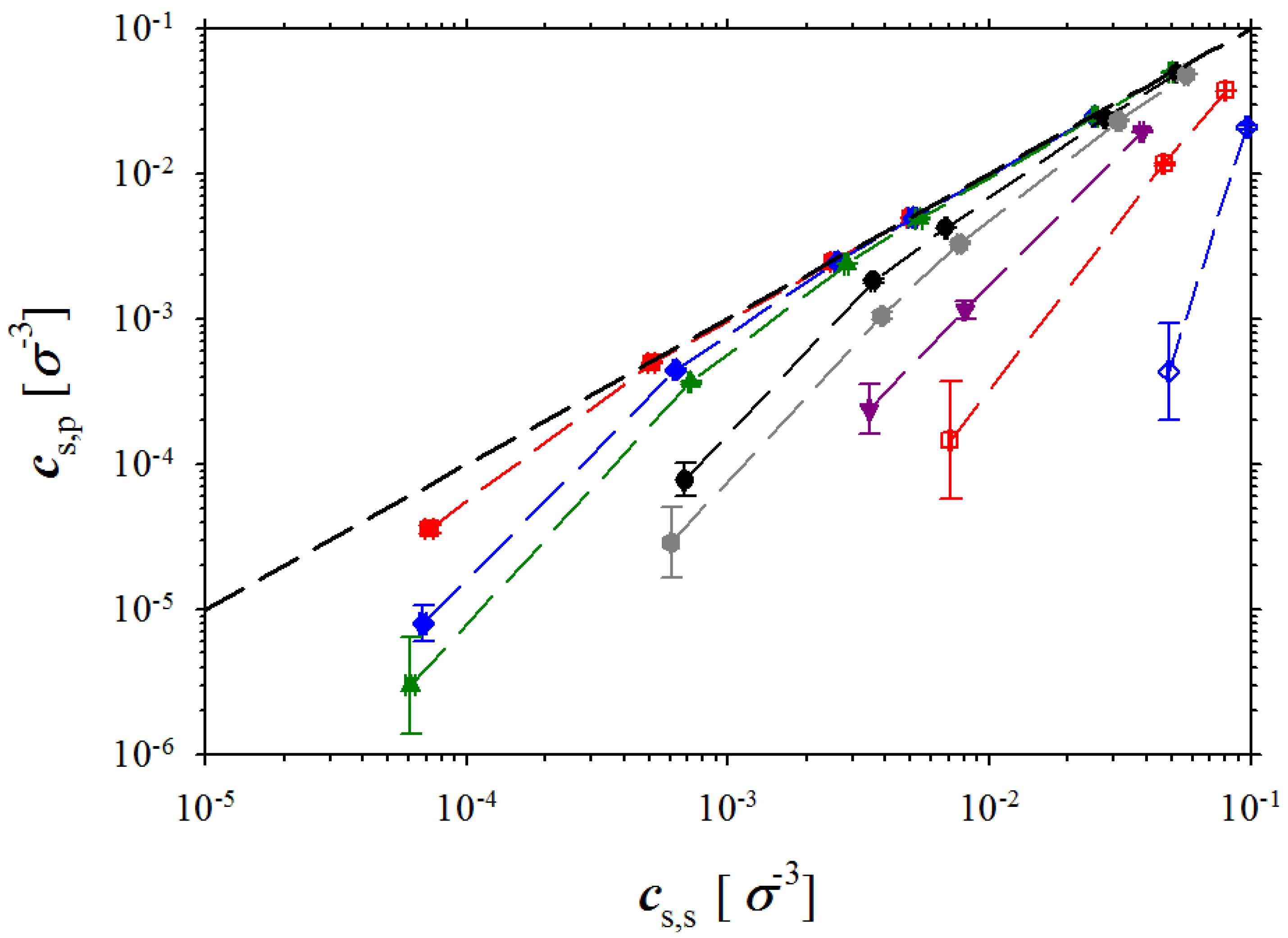
To obtain osmotic pressure of polyelectrolyte solutions we have performed hybrid Monte Carlo/molecular dynamics simulations [
33] of the counterions and salt ions exchange between two simulation boxes: one containing only salt ions (salt reservoir) and another filled with polyelectrolyte chains, counterions and salt ions (polyelectrolyte solution) (see
Figure 1). In our simulations polyelectrolytes were modeled by chains of charged Lennard-Jones (LJ) particles with diameter σ and degree of polymerization
N = 300 [
23,
32,
34,
35]. Each monomer on the polymer backbone was positively charged. Counterions and salt ions were modeled as LJ-particles with diameter σ. The solvent was treated implicitly as a dielectric medium with the dielectric constant ε.
Figure 1.
Snapshots of the simulation boxes containing salt solutions of polyelectrolyte chains (left) and salt (right).
Figure 1.
Snapshots of the simulation boxes containing salt solutions of polyelectrolyte chains (left) and salt (right).
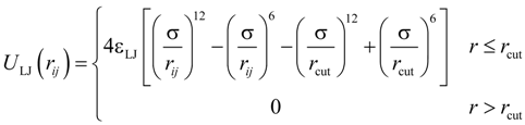
All particles in the system interacted through truncated-shifted Lennard-Jones (LJ) potential:
where
rij is the distance between
i-th and
j-th beads, and σ is the bead diameter chosen to be the same regardless of the bead type. The cutoff distance,
rcut = 2.5σ, was set for polymer–polymer interactions, and
rcut = 2
1/6σ was selected for all other pair wise interactions. The interaction parameter ε
LJ was equal to
kBT for polymer-ion, and ion-ion interactions, where
kB is the Boltzmann constant and
T is the absolute temperature. The value of the Lennard-Jones interaction parameter for the polymer–polymer pairs was set to 0.3
kBT which is close to a theta solvent condition for the polymer backbone.
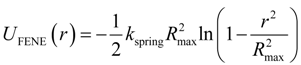
The connectivity of monomers into polymer chains was maintained by the finite extension nonlinear elastic (FENE) potential:
with the spring constant
kspring = 30
kBT/ σ
2 and the maximum bond length ,
Rmax = 1.2σ. The repulsive part of the bond potential was represented by the truncated-shifted LJ potentials with ε
LJ = 1.5
kBT and
rcut = 2
1/6σ.
Interaction between any two charged particles with charge valences
qi and
qj, and separated by a distance
rij, was given by the Coulomb potential:
Where
lB =
e2/ε
kBT is the Bjerrum length. In our simulations, the value of the Bjerrum length
lB was equal to 1.0σ. The Particle-Particle Particle-Mesh (PPPM) method implemented in LAMMPS [
36] with the sixth order charge interpolation scheme and estimated accuracy 10
−5 was used for calculations of the electrostatic interactions between all charges in each simulation box.
The snapshots of the simulation boxes are shown in
Figure 1. The salt box had dimensions 368.4 × 368.4 × 368.4σ. The system dimensions, number of polyelectrolyte chains, counterions, salt ions and box sizes of polyelectrolyte solution box were the same as in our previous publication with the initial number of particles varying between 24,000 and 36,000 [
32]. We covered the polymer and salt concentration range between 10
−5 σ
−3 and 0.1 σ
−3. Conversion of the reduced units to moles per liter is given at the end of this section.
Simulations were carried out with periodic boundary conditions for each simulation box. The total number of particles in both simulation boxes and their volumes remained constant during the entire simulation runs. We have only allowed exchange of the small ions between two simulation boxes. To perform these simulations, we have modified LAMMPS code by calling molecular dynamics steps as subroutines between Monte Carlo steps that were used to perform the exchange of small ions between two simulation boxes.
In order to maintain a constant temperature of the system during molecular dynamics simulation steps, we coupled each simulation box to the Langevin thermostat. The motion of particles (monomers, counterions, and salt ions) was described by the following equations:
where
m is the particle mass,
![Polymers 06 01897 i014]()
is the particle velocity, and
![Polymers 06 01897 i015]()
denotes the net deterministic force acting on the
i-th bead. The stochastic force
![Polymers 06 01897 i016]()
has a zero average value
![Polymers 06 01897 i017]()
and σ-functional correlation
![Polymers 06 01897 i018]()
. The friction coefficient ξ was set to ξ = 0.143
m/τ
LJ, where τ
LJ is the standard LJ-time τ
LJ = σ(m/
kBT)
1/2. The velocity-Verlet algorithm with a time step ∆t = 0.01τ
LJ was used for integration of the equations of motion Equation 4. The duration of the molecular dynamics simulation runs between Monte Carlo steps was 100 integration steps.
During Monte Carlo simulation steps, acceptance or rejection of the Monte Carlo moves followed a standard particle exchange procedure [
33]. The new configuration was obtained from the old configuration by removing one negatively and one positively charged ion from box 1 and inserting these particles into box 2. We alternate moves of the small ions in and out of the simulation box with polyelectrolyte chains. The detailed balance condition for these moves results in the following acceptance rule:
Where
![Polymers 06 01897 i019]()
are numbers of positively or negatively charged ions in the
i-th simulation box before the particle removal/insertion and ∆
U is the energy difference between total system energy in new and old configurations. It is important to point out that we considered negatively charged salt ions and counterions as indistinguishable for the ion exchange moves.
The simulations were performed according to the following procedure. At the beginning of each simulation run, both boxes contained salt ions at the same concentrations. For initial configuration of the simulation box with polyelectrolyte chains, we have used one of the system configurations from our simulations of polyelectrolytes in salt solutions [
32]. Then, we performed hybrid Monte Carlo/molecular dynamics simulation runs.
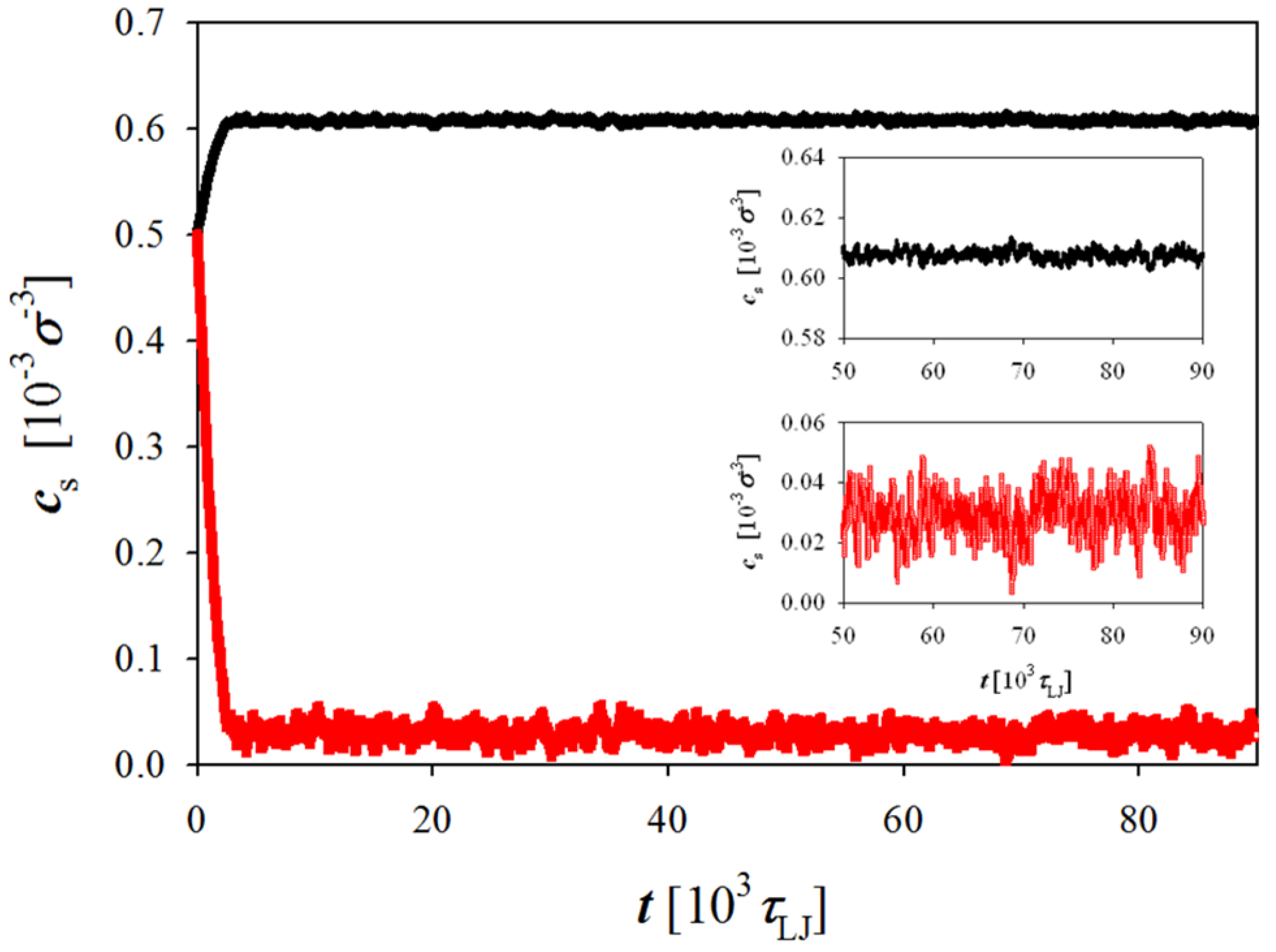
Figure 2 shows evolution of the salt concentration in simulation boxes representing polyelectrolyte solution and salt reservoir during the simulation run. As one can see, the salt concentration rapidly reaches an equilibrium value. Thus, the ion exchange between two simulation boxes is not a limiting step in achieving equilibrium. The duration of the simulation runs was varied between 6 × 10
4 τ
LJ and 10
5 τ
LJ depending on how long it required for the mean-square radius of gyration of a polyelectrolyte chain to reach equilibrium. Note that the system’s pressure equilibrates much faster, ~10
4 τ
LJ, than it requires for the chain equilibration (see SI). We used data collected during the final 2 × 10
4 τ
LJ for the data analysis. It is important to point out that the equilibrium bulk (reservoir) salt concentration was obtained after the equilibrium ion concentrations in both simulation boxes were reached.
Figure 2.
Evolution of concentration of the negatively charged salt ions in simulation box with (red line) and without (black line) polyelectrolyte chains during the simulation run. Simulations were performed at polymer concentration cp = 0.01 σ−3.
Figure 2.
Evolution of concentration of the negatively charged salt ions in simulation box with (red line) and without (black line) polyelectrolyte chains during the simulation run. Simulations were performed at polymer concentration cp = 0.01 σ−3.
In our simulations, we used a coarse grained representation of the polymers and salt ions. One of the possible mappings of our systems to a real system can be done by making a connection through the value of the Bjerrum length,
lB. In aqueous solutions at normal conditions, the value of the Bjerrum length is 0.7 nm. In our simulations, we set the value of the Bjerrum length to be equal to the LJ-diameter σ. Therefore, for the studied salt concentration range between 10
−5 σ
−3 and 0.1 σ
−3, the value of the Debye screening length due to only salt ions,
rD ≡ (8π
lBc
s)
−1/2, is varied between 44 nm and 0.44 nm. Using the relation between the solution ionic strength and the Debye radius,
![Polymers 06 01897 i020]()
, we can express studied concentration range in terms of moles per liter as follows 5 × 10
−5M < c
s < 0.5
M.
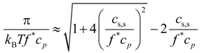
Figure 3.
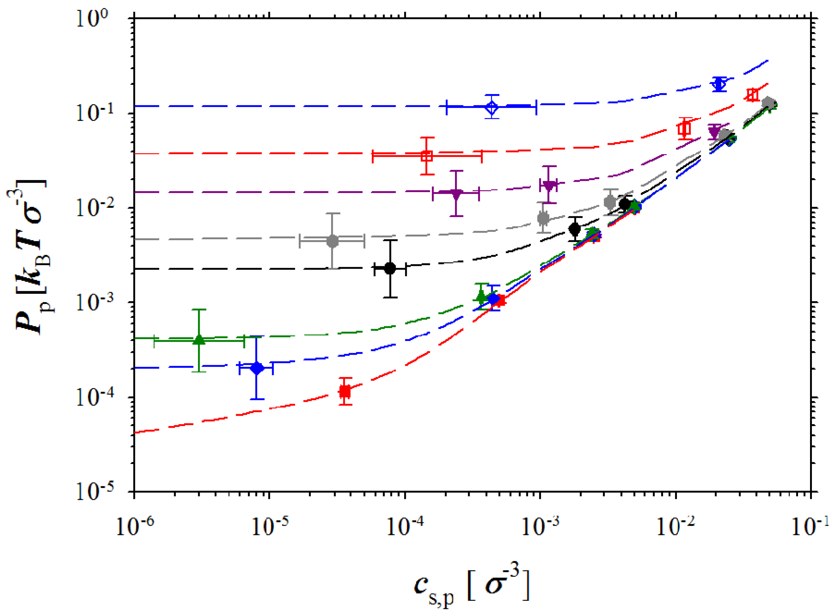
Dependence of the pressure in polyelectrolyte box on salt concentration in this box
cs,p for polyelectrolyte solutions with polymer concentrations
cp = 10
−4 σ
−3 (red squares),
cp =5 × 10
−4 σ
−3 (blue rhombs),
cp = 10
−3 σ
−3 (green triangles),
cp = 5 × 10
−3 σ
−3 (black circles),
cp = 10
−2 σ
−3 (gray hexagons),
cp = 2.5 × 10
−2 σ
−3 (purple triangles),
cp = 5 × 10
−2 σ
−3 (open red squares), and
cp = 10
−1 σ
−3 (open blue rhombs). The dashed lines correspond to the best fit to the data obtained in simulations without ion exchange using Sigma plot’s smooth spline method [
32].
Figure 3.
Dependence of the pressure in polyelectrolyte box on salt concentration in this box
cs,p for polyelectrolyte solutions with polymer concentrations
cp = 10
−4 σ
−3 (red squares),
cp =5 × 10
−4 σ
−3 (blue rhombs),
cp = 10
−3 σ
−3 (green triangles),
cp = 5 × 10
−3 σ
−3 (black circles),
cp = 10
−2 σ
−3 (gray hexagons),
cp = 2.5 × 10
−2 σ
−3 (purple triangles),
cp = 5 × 10
−2 σ
−3 (open red squares), and
cp = 10
−1 σ
−3 (open blue rhombs). The dashed lines correspond to the best fit to the data obtained in simulations without ion exchange using Sigma plot’s smooth spline method [
32].
3. Discussion and Simulation Results
We first will discuss pressure dependence on the polymer and salt concentrations in a simulation box containing polyelectrolyte chains. These data are presented in
Figure 3 that shows how pressure
Pp in polyelectrolyte solutions depends on equilibrium salt concentration
cs,p at different polymer concentrations,
cp. The error bars for all our figures were calculated by using standard definition of the variance σ
A of the quantity
A,
![Polymers 06 01897 i021]()
, which values were obtained during the production runs. This gives us the upper bound for the error estimate [
33]. Utilization of the block averaging procedure [
33] for evaluation of the variance of mean could decrease size of the error bars at least by a factor of three (see SI). (A comment has to be made here, since in our simulations the solvent was considered as a dielectric continuum, that the calculated system pressure for each simulation box corresponds to an osmotic pressure measured across a membrane which is only permeable to solvent molecules.) There are two different regimes in the pressure dependence on the salt concentration. At low salt concentrations, the pressure in the simulation box does not depend on salt concentration and saturates. The saturation level increases with increasing polymer concentration. However, at high salt concentrations, all pressure curves converge approaching a linear dependence on salt concentration. The crossover between high and low salt concentration regimes shifts towards high salt concentrations with increases in the polymer concentration. It is important to point out that this behavior of the system pressure is identical to that observed in our previous simulations corresponding to a system without salt ion exchange. To further highlight this fact, we show the lines representing the best fit to simulation results of the molecular dynamics simulations of the polyelectrolyte solutions without ion exchange [
32]. We can utilize our previous results [
32] and define a fraction of the osmotically active counterions or counterion activity coefficient as follows:
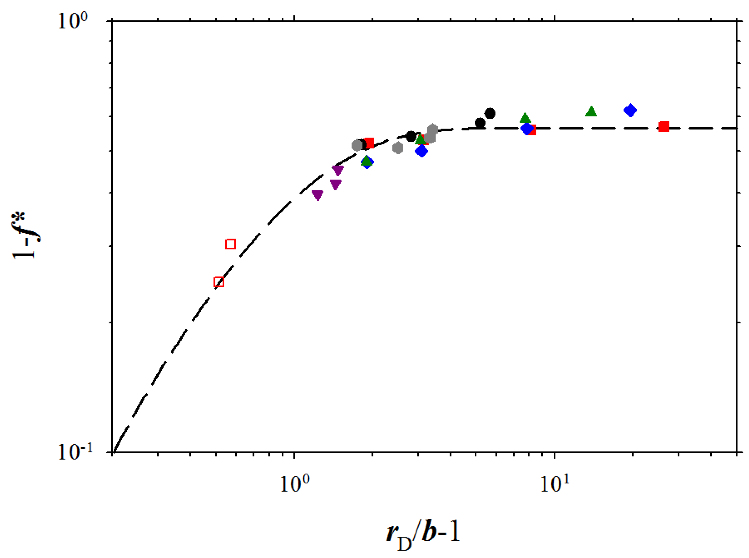
As we have already pointed out in our previous paper, the definition of the fraction of osmotically active counterions given by Equation 6 is only warranted in the concentration range where the pressure of the polyelectrolyte solutions is dominated by the linear term in the virial expansion. Analysis of the pressure data shows that we can represent the fraction of the condensed counterions (osmotically inactive counterions) 1
− f* in terms of the ratio of the Debye screening length:
to the average bond length
b (see
Figure 4). Note, that in definition of the Debye screening length we only included osmotically active counterions by multiplying counterion concentration by the activity coefficient,
f*. As one can see from
Figure 4, there is a wide interval of polymer and salt concentration where fraction of the condensed counterions saturates and is almost concentration independent. The invariance of the fraction of the condensed counterions, 1 −
f*, with solution ionic strength (plateau regime in
Figure 4) is in agreement with the osmotic pressure data for NaPSS [
5,
6,
10] and DNA [
12] solutions. However, at high solution ionic strengths
I (small values of the Debye screening length) the fraction of the condensed counterions increases linearly with increasing the value of the Debye screening length. Following our previous analysis of the simulation data, without ion exchange, we can fit all simulation data points by a function:
The agreement between fitting function and simulation results is reasonably good in the entire interval of the studied ionic strengths.
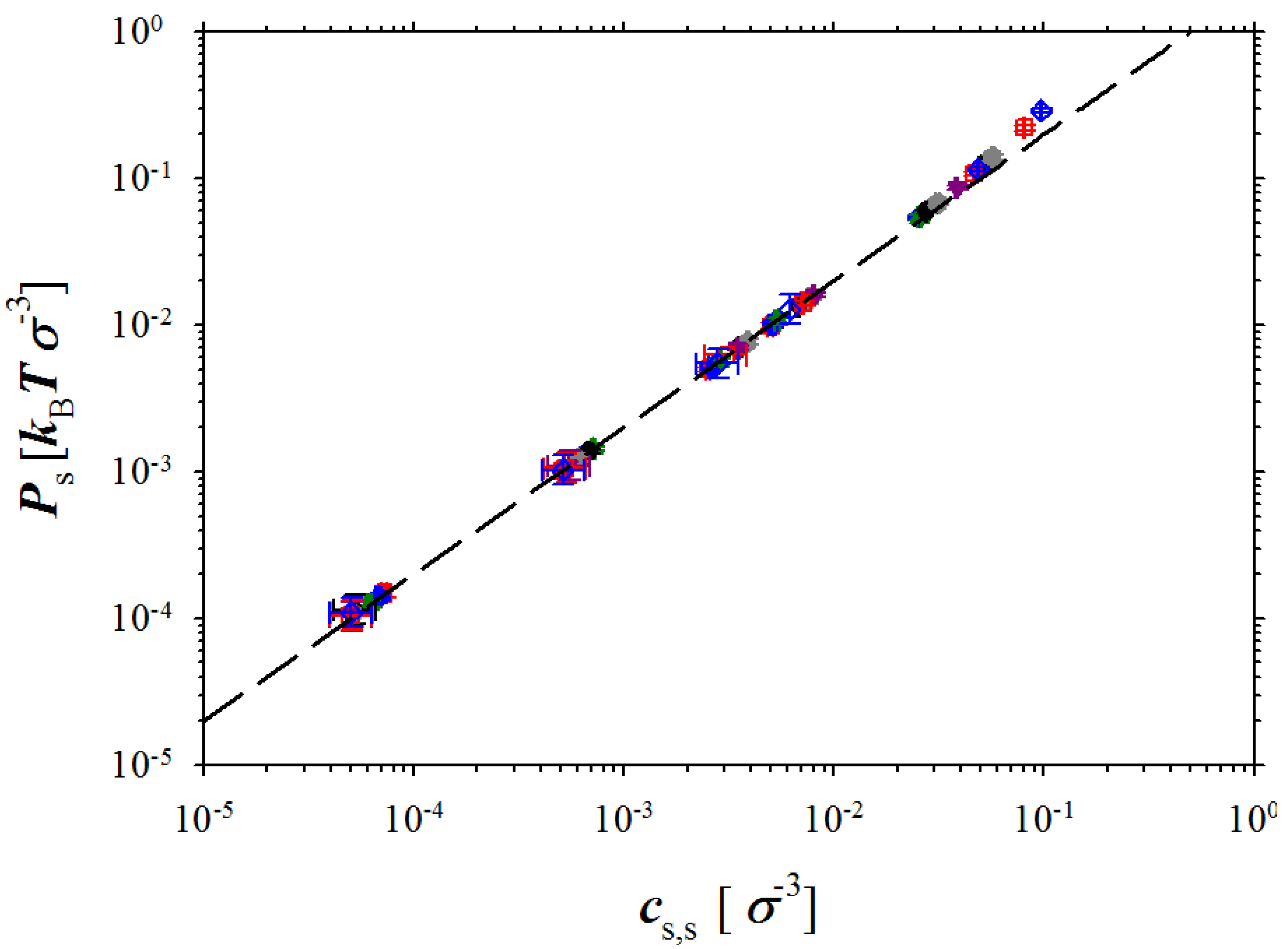
Now let us turn our attention to the salt reservoir.
Figure 5 shows dependence of the pressure in the salt simulation box on the salt concentration
cs,s. It follows from this figure that almost all our simulation data correspond to ideal solution regime where system pressure scales linearly with salt concentration. The deviation from the linear regime occurs at salt concentrations
cs,s > 5 × 10
−2 σ
−3. At these salt concentrations, the short range interactions between ions (excluded volume terms) begin to contribute to the system pressure. Our simulations also indicate that similar behaviour of the osmotic pressure should be expected for a wide concentration range up to salt and polymer concentrations of 0.1 M (see unit conversion at the end of
Section 2).
Figure 4.
Dependence of fraction 1 −
f* of the condensed counterions on the ratio of the Debye screening length to the bond length,
rD/
b, for polyelectrolyte solutions of chains with the degree of polymerization
N = 300. The dashed line is the best fit to Equation 8 with the values of the fitting parameters:
A = 0.566,
B = 1.26. The data points correspond to polymer concentrations c
p ≤ 0.05σ
−3 and salt concentrations c
s,
p < 0.05σ
−3. Notations are the same as in
Figure 3.
Figure 5.
Dependence of the pressure in salt box on salt concentration. The dashed line is given by the following equation Ps = 2kBTcs,s.
Figure 5.
Dependence of the pressure in salt box on salt concentration. The dashed line is given by the following equation Ps = 2kBTcs,s.
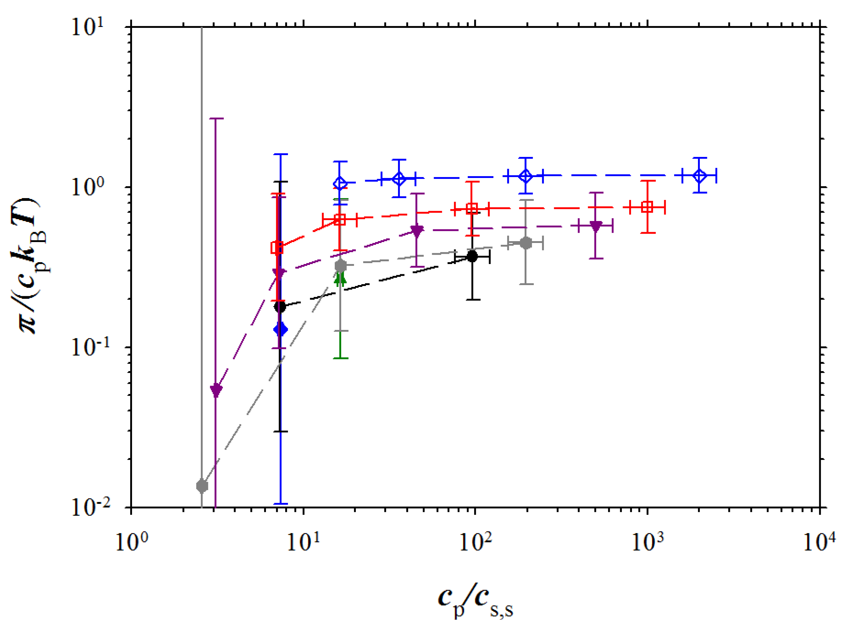
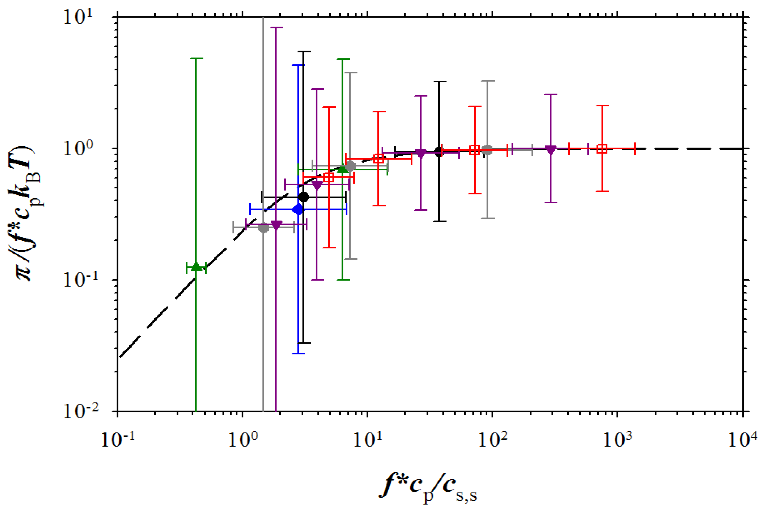
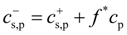
Osmotic pressure is defined as a difference between pressure of polyelectrolyte solution and salt reservoir:
Figure 6 shows dependence of the osmotic coefficient π/(
cpksT) on the ratio of the polymer concentration and salt concentration in salt reservoir. The osmotic coefficient first increases with increasing the concentration ratio then saturates. The magnitude of the saturation plateau increases with increasing polymer concentration. It is well known that this value corresponds to the fraction of the osmotically active counterions in low salt concentration regime (see for review [
2,
9,
10]). Note, that the large error bars seen in this figure is a manifestation of the fact that the osmotic pressure is a difference between pressure of polyelectrolyte solution and salt reservoir (see Equation (9)).
Figure 6.
Dependence of the osmotic coefficient on the reduced polymer concentration. Notations are the same as in
Figure 3.
Figure 6.
Dependence of the osmotic coefficient on the reduced polymer concentration. Notations are the same as in
Figure 3.
Since the majority of our simulations corresponds to a ion concentration range where the contribution of ions can be taken into account in the framework of the ideal gas approximation, we can test how well the classical Donnan equilibrium approach [
4,
10] describes our simulation results. In the ionic systems, the Donnan equilibrium requires charge neutrality on both sides of the membrane across which the osmotic pressure π is measured. The electroneutrality condition leads to partitioning of salt ions between the reservoir and polyelectrolyte solution:
Note that in our simulations, polyelectrolyte chains were positively charged (see
Section 2); therefore, concentration
![Polymers 06 01897 i022]()
also includes contribution from osmotically active counterions. The local ion concentrations
cs+(
r) and
cs−(
r) are related to the local value of the electrostatic potential φ(
r) by the Boltzmann distribution:
In writing Equation (11), we set the value of the electrostatic potential in salt reservoir to zero. It follows from Equation (11) that the product of the concentrations of salt ions stays constant at each point of the solution. Our simulations are done at constant chemical potential which requires that this product stays constant in the salt reservoir as well. This leads to:
By solving Equations (10) and (12), we can find the average concentration of the positively and negatively charged salt ions in polyelectrolyte solution as a function of the average salt concentration
cs,s in salt reservoir and polymer concentration
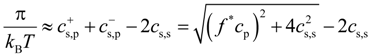
cp. The ionic contribution to the osmotic pressure is equal to the difference between the ideal gas pressure of salt ions in the polyelectrolyte solution and in the salt reservoir:
In the limit of low salt concentrations,
cs,s <<
f*c, this difference is proportional to the pressure from the ideal gas of osmotically active counterions,
kBTf*cp. At higher salt concentrations,
cs,s >>
f*cp, the ionic part of the osmotic pressure is equal to:
and can be considered as a result of the effective excluded volume interactions between charged monomers on the polyelectrolyte backbone. Note that at high salt concentrations, the concentration of the salt ions in salt reservoir and polyelectrolyte solution are close to each other. This is confirmed by
Figure 7 showing dependence of the salt concentration in polyelectrolyte solution as a function of the salt concentration in the salt reservoir.
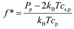
Equation (13) can be transformed into universal form as follows:
This allows us to collapse all simulation data sets shown in
Figure 6 into one universal plot (see
Figure 8). For this plot, we used the value of the fraction of osmotically active counterions
f* from
Figure 4. The errors in determining system osmotic pressure increase in simulations of solutions at high salt concentration regime where salt concentrations in both simulation boxes are close to each other (see
Figure 7). In this case, the pressure in both boxes is dominated by salt ions and osmotic pressure is obtained as a difference between two close values. To increase accuracy in determining this small difference, one has to perform simulations of the much larger systems to decrease errors in determining pressure in both simulation boxes.
Figure 7.
Dependence of salt concentration in polyelectrolyte solution on salt concentration in reservoir. Notations are the same as in
Figure 3.
Figure 7.
Dependence of salt concentration in polyelectrolyte solution on salt concentration in reservoir. Notations are the same as in
Figure 3.
Figure 8.
Universal plot of the system osmotic coefficient as a function of the reduced polymer concentration. Dashed line corresponds to Equation (15) with no adjustable parameters. Notations are the same as in
Figure 3.
Figure 8.
Universal plot of the system osmotic coefficient as a function of the reduced polymer concentration. Dashed line corresponds to Equation (15) with no adjustable parameters. Notations are the same as in
Figure 3.
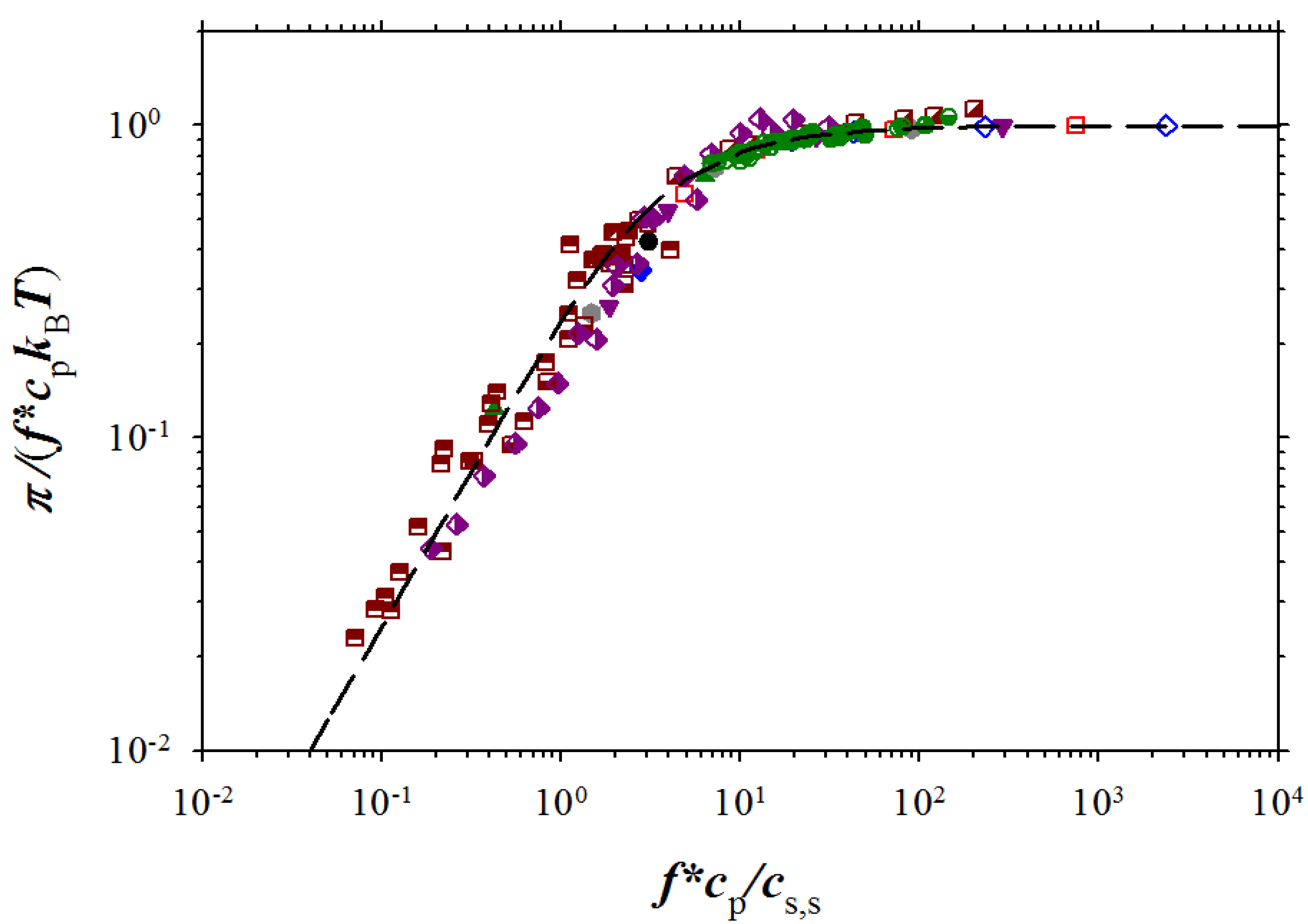
Despite the large error bars, our simulations show universality of the reduced osmotic coefficient as a function of the ratio of the concentration of the osmotically active counterion to the salt concentration in salt reservoir. In
Figure 9, we combined our simulation results and experimental data on sodium polystyrene sulfonate (NaPSS) [
5,
6], DNA [
12], sodium polyacrylate (NaPAA) [
27], polyacrylic acid (PA) [
26], polyvinylbenzoic acid (PVB) [
26], sodium polyanetholesulfonic acid (NaPASA) [
27], and polydiallyldimethylammonium chloride (PDADMA-Cl) [
27]. For this plot, we used for the fraction of the osmotically active counterions,
f*, as a fitting parameter throughout the entire salt and polymer concentration range. This procedure resulted in
f* = 0.16 for NaPSS [
10] and
f* = 0.24 for DNA [
12]. The fraction of the osmotically active counterions and residual salt concentrations for the salt-free data of Zhang
et al. [
27] and Kakehashi
et. al. [
26] were obtained by fitting the data to Equation (14). This fitting procedure resulted in
f* = 0.54
cs = 7.6 × 10
−3 M for NaPAA,
f* = 0.65
cs = 1.7 × 10
−2 M for NaPASA, and
f* = 0.6
cs = 5.2 × 10
−3 M for PDADMA-Cl. For Kakehashi et al. [
26] data for PA and PVB these parameters are
f* = 0.33
cs = 9.7 × 10
−3 M and
f* = 0.4
cs = 1.3 × 10
−2 M, respectively. As one can see from
Figure 9, the agreement between our simulation results and experiments is very good.
Figure 9.
Dependence of the reduced osmotic coefficient on the ratio of concentration of osmotically active counterions and salt ions. NaPSS data are from Takahashi
et al. [
5] (brown squares with filled right bottom corner), and Koene
et al. [
6] for
Mw = 4 × 10
5 g/mol (brown squares with filled left top corner),
Mw = 6.5 × 10
5 g/mol (brown squares with filled top), and
Mw = 1.2 × 10
6 g/mol (brown squares with filled bottom). DNA data (purple rhomb with filled right side) are from Raspaud
et al. [
12], NaPAA data (green circle with filled right side) and PDADMA-Cl data (green circles with filled bottom) are from Zhang
et al. [
27], and polyacrylate (PAA) data (green circle with filled left side) and PVB (green circle with cross) are from Kakehashi
et al. [
26]
. Symbols used for simulation data are the same as in Figure 3. Dashed line corresponds to Equation (15).


 is the particle velocity, and
  denotes the net deterministic force acting on the i-th bead. The stochastic force
  has a zero average value
  and σ-functional correlation
  . The friction coefficient ξ was set to ξ = 0.143m/τLJ, where τLJ is the standard LJ-time τLJ = σ(m/kBT)1/2. The velocity-Verlet algorithm with a time step ∆t = 0.01τLJ was used for integration of the equations of motion Equation 4. The duration of the molecular dynamics simulation runs between Monte Carlo steps was 100 integration steps.
 are numbers of positively or negatively charged ions in the i-th simulation box before the particle removal/insertion and ∆U is the energy difference between total system energy in new and old configurations. It is important to point out that we considered negatively charged salt ions and counterions as indistinguishable for the ion exchange moves.
 , we can express studied concentration range in terms of moles per liter as follows 5 × 10⁻⁵M < cs < 0.5M.
 , which values were obtained during the production runs. This gives us the upper bound for the error estimate [33]. Utilization of the block averaging procedure [33] for evaluation of the variance of mean could decrease size of the error bars at least by a factor of three (see SI). (A comment has to be made here, since in our simulations the solvent was considered as a dielectric continuum, that the calculated system pressure for each simulation box corresponds to an osmotic pressure measured across a membrane which is only permeable to solvent molecules.) There are two different regimes in the pressure dependence on the salt concentration. At low salt concentrations, the pressure in the simulation box does not depend on salt concentration and saturates. The saturation level increases with increasing polymer concentration. However, at high salt concentrations, all pressure curves converge approaching a linear dependence on salt concentration. The crossover between high and low salt concentration regimes shifts towards high salt concentrations with increases in the polymer concentration. It is important to point out that this behavior of the system pressure is identical to that observed in our previous simulations corresponding to a system without salt ion exchange. To further highlight this fact, we show the lines representing the best fit to simulation results of the molecular dynamics simulations of the polyelectrolyte solutions without ion exchange [32]. We can utilize our previous results [32] and define a fraction of the osmotically active counterions or counterion activity coefficient as follows:


 also includes contribution from osmotically active counterions. The local ion concentrations cs+(r) and cs−(r) are related to the local value of the electrostatic potential φ(r) by the Boltzmann distribution: