Phase Diagrams for Systems Containing Hyperbranched Polymers

Abstract
:Symbols
| b | Number of branching points |
| C | Contributions to the Helmholtz energy within the lattice cluster theory |
| D | Corrections to the Flory–Huggins theory, connectivity factor (Equation (20)) |
| E | Internal energy |
| F | Helmholtz energy |
| f | Mayer functions |
| G | Gibbs energy |
| g | Generation number |
| H | Enthalpy or summands in Equation (37) |
| I, J | Summands in Equation (38) |
| J | Grand thermodynamic potential |
| K, L, M | Factors describing the architecture of the polymer, defined in Equations (78,79) |
| K | Ratio of nearest-neighbour positions with a proper orientation to all possible orientations |
| k | Interaction parameter (Equation (91)) |
| M | Molecular weight or number of segments |
| m | Number of chains in the system |
| N | Topological coefficient (Table 1) or number of lattice sites |
| n | Amount of mole |
| P | Pressure |
| p | Counting variable |
| Q | Summands in Equation (41) |
| r | Position of the segments |
| S | Entropy |
| T | Temperature |
| u | Interaction potential |
| V | Volume |
| v | Specific volume |
| W | Microcanonical partition function |
| w | Mass fraction |
| X | Mole fraction |
| Z | Partition function |
| z | Coordination number |
Superscript
| a, b | Phase a or b |
| ath | Athermic mixture |
| LV | Liquid-vapour equilibrium |
| MF | Mean field approach |
| reg | Regular mean field energetic contribution |
Subscript
| Ai | Non-bonded segment to the association site A |
| asso | Association |
| att | Attractive part of the interaction potential |
| B | Boltzmann constant |
| CH | Solvent cyclohexane |
| comp | Pure compound |
| FH | Flory–Huggins theory |
| i | Component i or counting variable |
| l | Lattice |
| LCT | Lattice cluster theory |
| Polymer | Polymer |
| R | Repulsive part of the interaction potential |
| v | Void lattice site |
Creek letters
 | Flory–Huggins interaction parameter |
 | Factor in the polynomial series in Equation (29) |
 | Vector pointing to the next neighbour |
 | Difference or association strength |
 | Kronecker Delta function |
 | Interaction energy |
 | Volume fraction |
 | Segment molar fraction |
 | Corrections to the Flory–Huggins theory, combinatorial factor (Equation (20)) |
 | Association volume in the original Wertheim theory |
 | Chemical potential |
 | Density |
 | Length of a cubic cell |
1. Introduction
2. Theory
2.1. Phase Equilibrium Thermodynamics
2.1.1. Ensembles and Potentials
 (1)
(1) (2)
(2) (3)
(3) , volume
  , temperature
  , amount of substance
  ,
,  , and the chemical potentials of the components ,
  . The derivatives of the respective potentials, with respect to their natural variables, yield all other thermodynamic information. For example the derivative of Helmholtz energy with respect to volume results in the negative system pressure,
  :
: (4)
(4) (5)
(5) and
and  are the respective potentials and
  is one of the natural variables of potential, . The list of common transformations is shown below.
 (6)
(6) (7)
(7) (8)
(8) (9) , Helmholtz free energy
  , Gibbs energy
  and enthalpy
  .
.2.1.2. Phase Equilibrium Calculations
 and
and  the Helmholtz free energy and the Gibbs energy are of substantial importance. Both these potentials do have a minimum in equilibrium. This means, an optimization approach to the calculation of equilibria is feasible.
 (10)
(10) (11)
(11) (12)
(12) (13)
(13) (14)
(14) equations or
  equations for a compressible system, where is the number of components.
2.1.3. Flory–Huggins Theory
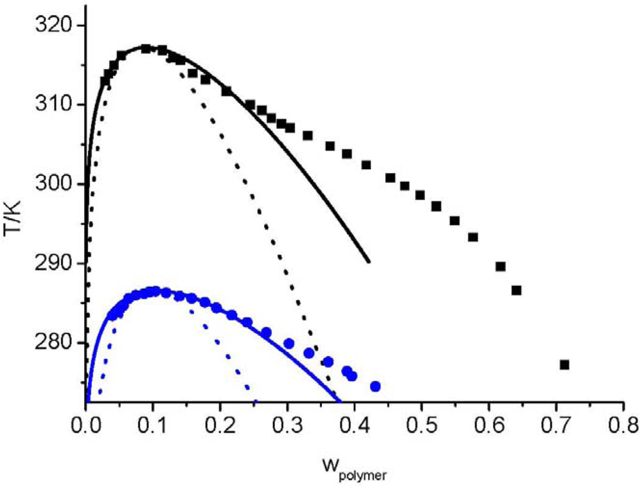
 is examined. Here, the mole fraction of the polymer approaches zero implying that Raoult’s law [104] is applicable for the solvent, yet the mixture is highly non-ideal. Figure 1 demonstrates an impressive example, namely the vapour pressure of a polymer solution. According to Raoult’s law, the vapour pressure of the considered solution should change linearly (straight line in Figure 1) from the vapour pressure of the solvent to zero pressure, because the vapour pressure of the pure polymer is zero. However, the experimental data, taken from the literature [61], are far away from Raoult’s law. Additionally, the experimental data in Figure 1 clearly shows the impact of polymer architecture on the thermodynamic properties. Although the same type of polymer from the chemical point of view (linear and branched polyisoprene) in the same solvent (cyclohexane) was used, differences in the vapour pressure are found experimentally. These differences can only be explained by the influence of the chain architecture on the thermodynamic properties. The experimental results demonstrate that cyclohexane is a considerably worse solvent for branched polyisoprene than for the linear analog at all temperatures and at all compositions. This finding is in seeming contrast to the widespread notion that branched polymers are better soluble than their linear counterparts. It may, however, well be that special interactions between the components of the mixture and larger differences between the end groups and the middle groups of the polymer are capable to change the picture.
 , divided by the vapour pressure of the pure solvent
  , made from linear (black symbols) or branched (blue symbols) polyisoprene and cyclohexane [61].
, divided by the vapour pressure of the pure solvent , made from linear (black symbols) or branched (blue symbols) polyisoprene and cyclohexane [61].
, made from linear (black symbols) or branched (blue symbols) polyisoprene and cyclohexane [61].
, divided by the vapour pressure of the pure solvent , made from linear (black symbols) or branched (blue symbols) polyisoprene and cyclohexane [61].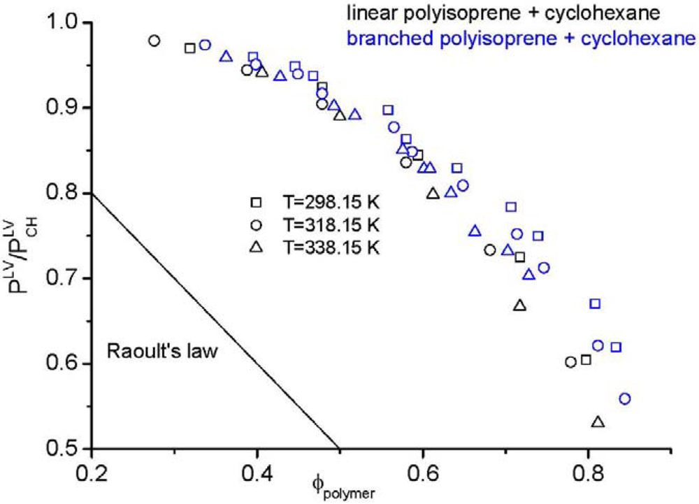

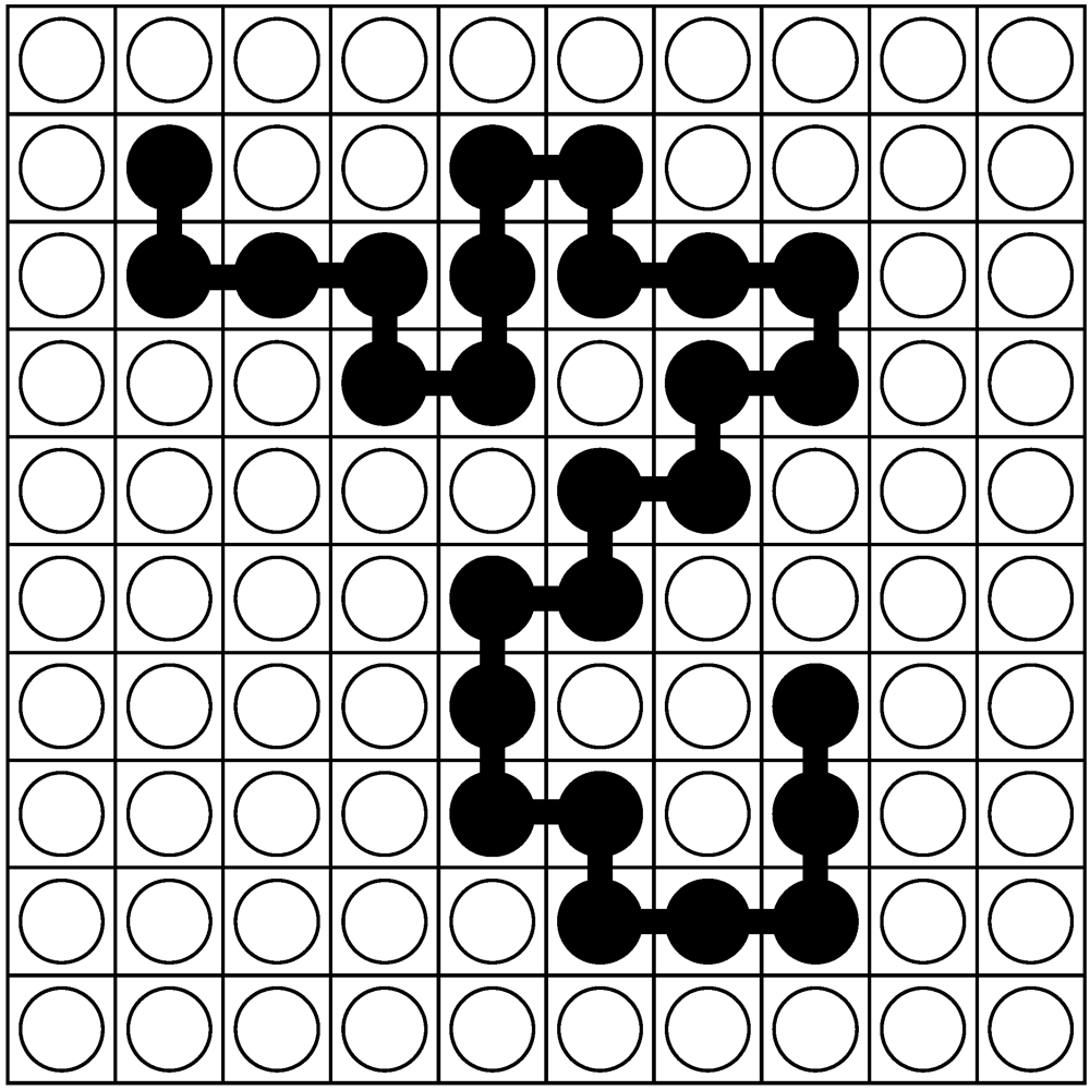
 of a system containing a solvent and a linear polymer, the number of ways to consecutively insert a polymer chain into a lattice of coordination number
  , at first fully occupied by solvent beads, must be calculated.
- (a) a polymer chain is composed of
![Polymers 04 00072 i051]() segments of equal size.
segments of equal size. - (b) the polymer segments size equals that of the solvent.
- (c) the polymer is inserted randomly, but can fill the lattice completely (i.e., forms a perfect crystal).
 (15)
(15) is the number of lattice sites,
  is the Boltzmann constant,
  is the number of segments the polymer is composed of,
  is the number of solvent segments, and the
  are the segment mole fractions of components , defined as:
 (16)
(16) (17)
(17) . By using Equation (7) the Helmholtz free energy is derived [84].
  (18) was introduced [81,82,83,84]. The approach, employed to calculate the phase behaviour of hyperbranched polymers, is the extension of FH theory based on physical argumentation.
 2.2. Lattice Cluster Theory
2.2.1. LCT of Incompressible Systems
and  interacts with the energy
  can be read as [92]:
 (19) is the Kronecker delta function and the vector is pointed from a given lattice site to the nearest neighbour lattice sites. A factor
  has to be introduced for the indistinguishability of polymer chains of the same species and the factor ½ accounts for the symmetry of each chain. The outside summation in Equation (19) prohibits any lattice site from being occupied by two polymer segments. In the outside summation of Equation (19) there are two factors, whereas the first factor accounts for the bonding constraints in the polymer, the second factor describes the Van der Waals interaction between two lattice sites. The expression in Equation (19) represents an exact solution of a component polymer blend on a cubic Bravais lattice, but for using this approach a simplification is desirable. In the FH theory this simplification is the assumption that just the next neighbours of one polymer segment have to be considered. Freed and Dudowicz [89] extend the assumption of the FH theory by the introduction of a cluster expansion. This expansion goes back to the cluster expansion introduced by Mayer [99] for non-ideal gases. In the framework of LCT, the corrections to the Helmholtz free energy are derived in form of a cluster series expansion in the inverse coordination number
  and in the reduced interaction energy
  , taking into account the growing correlations between near segments on the same molecule. component polymer blend reads as [89]:
 (20)
(20) as suggested by Freed and Dudowicz [89]. One example of evaluating the second order contribution such a diagram will be shown in the following.
 (21)
(21) (22)
(22) , which depends on the number of components and is independent of the polymer architecture. As an example the diagram k1 in Equation (22) is evaluated. For a one component system it is obtained:
 (23)
(23) and
and  are the number of two successive bonds in a single polymer chain and in that order the number of monomers of one chain, while
  is the number of chains in the system. The factor 1/5! arises because of the indistinguishability of selecting the chains.
 bonds [89]:
 (24) depends only on the number of lattice sites and the number of vertices in the diagram
  [ 89]. The factor
  depends only on the lattice, but not on the polymer architecture. The evaluation process is shown by Dudowicz and Freed [89]. By knowledge of the combinatorial factor and the connectivity factor, this diagram can be analysed. The evaluation leads to the contribution [89]:
 (25)
(25) is that of the compressible mixture:
 (26)
(26) (27)
(27) (28)
(28) (29)
(29) is the chain length of component . In Equation (29) the corrections to the FH theory appear in form of a power series. Its coefficients depending only on the polymer architecture, which is described with
  , and the interaction energy
  can be computed using the following relations [57]:
 (30)
(30) (31)
(31) (32)
(32) (33)
(33) (34)
(34) (35)
(35) only the parameters
  and
and  are left, which can be summarized to the well known Flory–Huggins parameter. To characterize the architecture of a molecule the geometric parameters (
  ) are important. These parameters will be explained in the section dealing with the application to hyperbranched polymers, but at first the Helmholtz free energy of a ternary solution will be introduced.
  (36)
(36) ), as well as the first (
  ) and second order (
  ) of energy can be calculated using the tables I, II and III published by Dudowicz and Freed [89] and taking into account the corrections introduced by Dudowicz et al. [110]. The entropic part of the Helmholtz free energy reads [56]:
  (37)
(37) and they can found in the literature [56]. ) as well as the second order mixing energy ( ) can be expressed as a sum [56]:
  (38)
(38) and
and  are given in literature [56]. These contribution depend on the architecture via
  and additionally from the difference in interaction energy of component and , expressed by the three interaction parameters
  ,
,  , and
, and  . In the z→∞ and ε→0 limit this theoretical framework reduces to the Flory–Huggins expression of a ternary polymer solution and it reduces also correctly to the equation describing a binary mixture (Equation (29)). For applying the LCT, the determination of the architectural parameters is necessary. This will be shown in Section 2.2.3.
2.2.2. LCT of Compressible Systems
 (39)
(39) (40)
(40) is the segment fraction of void lattice cells. The entropic contribution for pure components can be written as a polynomial in the void segment fractions [111,112]:
 (41) [111,112]:
 (42)
(42) (43)
(43) (44)
(44) (45)
(45) (46)
(46) (47)
(47) is the interaction energy between two segments of component . Again, the coefficients of the polynomial can be expressed in terms of the molecule’s structure and the lattice coordination number [111,112]:
 (48)
(48) (49)
(49) (50)
(50) (51)
(51) (52)
(52) (53)
(53) (54)
(54) (55)
(55) (56)
(56) (57)
(57) (58)
(58) (59)
(59) (60)
(60) (61)
(61) is the length of a cubic cell, a segment of molecule occupies. The specific volume of the substance can be calculated with the following equation:
 (62)
(62) (63)
(63) (64)
(64) was developed. The interaction energy difference between a segment and a void lattice site becomes
  , because of the vanishing energies
  and
and  . Using the same strategy discussed above leads to power series allowing the calculation of the Helmholtz energy and all other thermodynamic properties [111,112]. The formulation in terms of
  and the reformulation of the Helmholtz free energy reduces the number of terms necessary to calculate from 103 [89,90,91] to 21 [111,112]. All coefficients depend only on the species’ chemical architecture and the lattice coordination number. The component indices range from zero to the number of components present in the mixture , where zero is the index of voids.
2.2.3. Application to Hyperbranched Polymers
can be evaluated by counting the repeating unit of a polymer chain. Also the number of bonds  is independent of the polymers’ branching architecture and can be calculated as follows [113]:
 (65)
(65) , where describes the branching degree, that means the number of bonds which meet at one repeating unit.
| | Number of repeating units in a polymer chain |
| | Number of bonds in a polymer chain |
| | Number of two consecutive bonds in a polymer chain |
 | Number of three consecutive bonds in a polymer chain |
 | Number of four consecutive bonds in a polymer chain |
 | Number of distinct ways of selecting two non-sequential bonds on the same chain |
 | Number of distinct ways of selecting two sequential bonds and one non-sequential bond on the same chain |
 | Number of distinct ways of selecting two non-sequential double consecutive bonds on the same chain |
 | Number of ways in which three bonds meet at a lattice site for a polymer chain |
 | Number of ways in which four bonds meet at a lattice site for a polymer chain |
 | Number of ways in which three bonds meet at a lattice site for a polymer chain and one bond is at this lattice site |
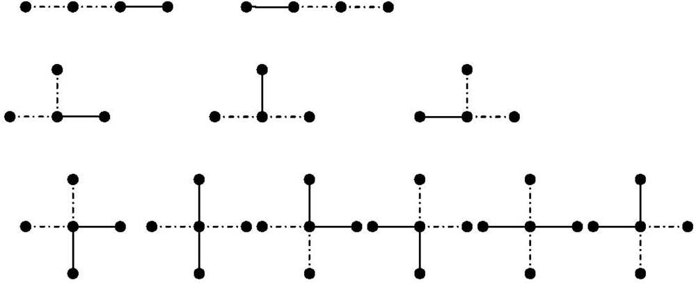
 (66) is the number of branching points of degree in which bonds meet. will be shown. For a linear polymer in Figure 3 (first row) with three bonds, there are two possibilities of choosing two consecutive bonds in a linear polymer with three bonds. The chosen bonds are marked by broken lines. This can be generalized for a linear polymer with monomers as follows [113]:
 (67)
(67) denotes for a linear chain.
 (68)
(68)
| Branching degree | Additional possibilities of choosing two consecutive bonds |
|---|---|
| 3 | 1 |
| 4 | 3 |
| 5 | 6 |
| 6 | 10 |
| 7 | 15 |
is reduced by each chosen bond and the factor 1/2 appears because of the indistinguishability. In an analogous manner the number of ways of choosing three or four bonds can be described [113]: (69)
(69) (70)
(70) describes the contribution of a linear chain [113]:
 (71)
(71) bonds meeting at one lattice site. As an example the number of three bonds meeting at one lattice site is derived.
| Branching degree | Ways of choosing three bonds at one lattice site |
|---|---|
| 3 | 1 |
| 4 | 4 |
| 5 | 10 |
| 6 | 20 |
| 7 | 35 |
 (72) is the number of points meeting at one lattice site which is reduced by one for each chosen bond and the factor 6 appears because of the indistinguishability. In a similar way the coefficient can be determined [113]:
 (73)
(73) (74) will be shown [113]:
 (75)
(75)
 (76)
(76) (77). With help of the presented parameters, the
  and the
  that occur in the incompressible version and
  for the compressible version can be calculated as follows:
 (78)
(78) (79)
(79) ;
;  ;
; 
 ;
;  ;
; 
 ;
;  ;
;  (80)
(80) [93].
[93].
[93].
[93].
 (Boltorn H20), (Boltorn H30) and
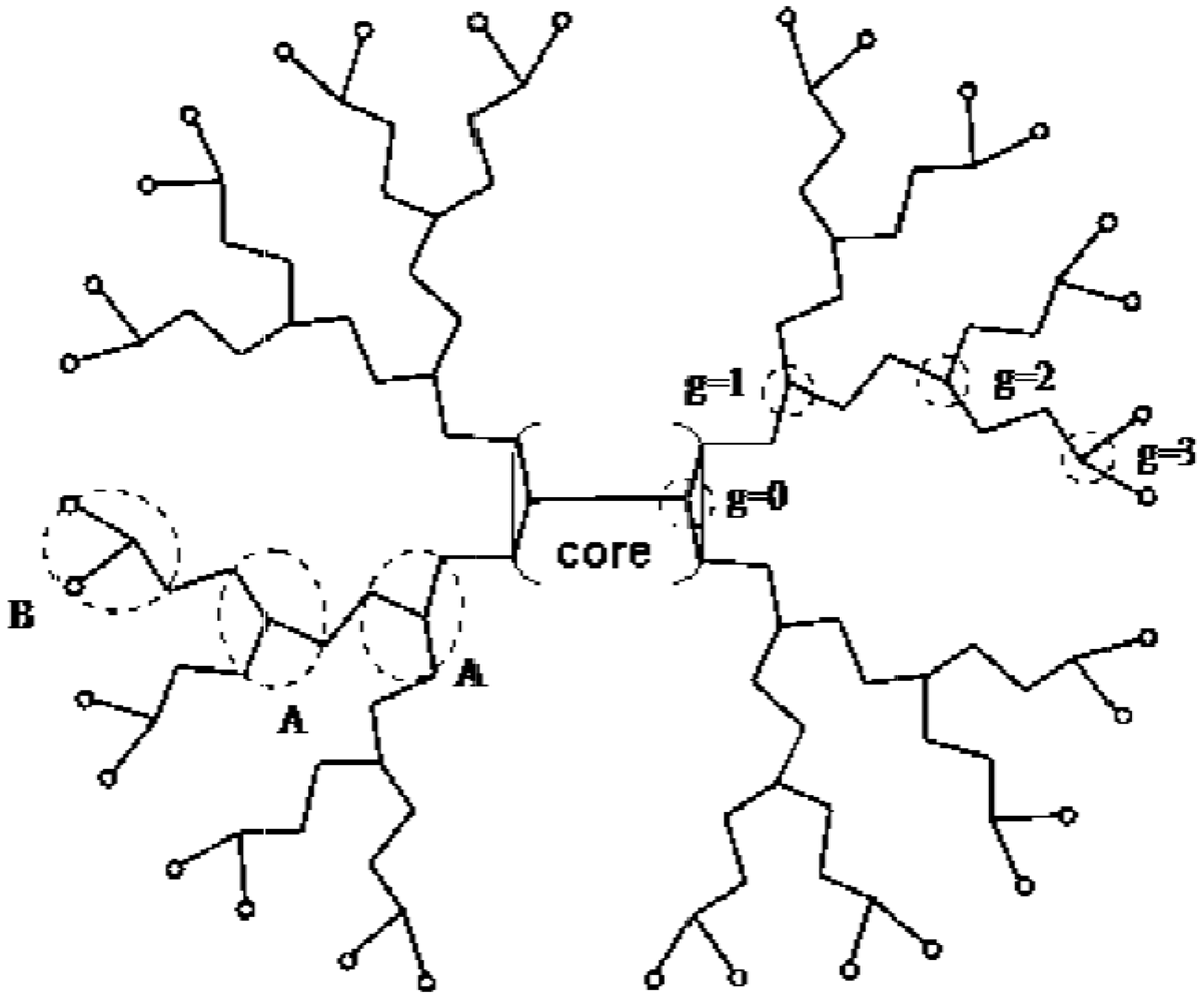
  (Boltorn H40) will be regarded [53]. All these molecules possess the same core: O[CH2C(C2H5)(CH2O–)2]2. Depending on the generation number g, the molecules additionally include a different number of groups A: COC(CH3)(CH2OH–)2. and B: COC(CH3)(CH2OH)2. The general formulae of the polymers are for g = 2:
  , for g = 3:
  and for g = 4:
  . According to these formulae (neglecting polydispersity) the molar masses take the values 1,642 g/mol (g = 2), 3,498 g/mol ( ) and 7,210 g/mol (g = 4). The number of OH– end groups equals the number of B-units. Figure 5 shows schematically a hyperbranched polyester with the generation number g = 3.
  will be used [53]. The separator length is the number of segments between two branching points. It denotes the number of segments of an A unit or a B unit. The number of core segments is given by the quantity,
  . It is assumed that one water molecule occupies one lattice site, so the number of core segments and the separator length can be determined by dividing the core, A and B units in groups that have a molar mass comparable to a water molecule. The values of the separator length, number of core segments and generation number are collected in Table 4.
| Separator length | 4 |
| Number of core segments | 7 |
| Generation number | (Boltorn H20) (Boltorn H30) (Boltorn H40) |
 (81)
(81) (82)
(82)2.3. Wertheim Theory
2.3.1. Derivation of the Association Theory
is divided into a density of non-bonded particles  and a density of particles
  forming an attractive bond with another particle [73]:
 (83)
(83) is constituted from contributions arising from the correlations between two particles which have not formed an attraction bond
  , two particles of which one has formed an attraction bond
  and
and  , and two particles that both have formed an attraction bond
  . The coordinates of particles 1 and 2 are given by
  and
and  , where
  denotes the position and
  the orientation of particle .
 depending on the orientation of particle 1 and 2 can be split in two parts, an isotropic repulsive part
  and a directional attractive part
  . The Mayer function
  can be divided in an attractive
  and a purely repulsive part
  [73]:
[73]: (84)
(84) (85)
(85) (86) in terms of the activity , fR- and F-bonds similar to LCT. According to the suggested expansion, the overall density is devided into densities of bonded and non-bonded particles. The and
  -values are then both classified by a different part of the set of diagrams that constitutes . Starting from the grand canonical partition function
  and applying these expansions of and , Wertheim [73,74] derived an exact diagrammatic expansion of the structural correlations , , and in terms of and , fR- and F-bonds. He then constituted, along the same lines as the direct correlation function is defined, for fluids consisting of hard spheres, partial direct correlation functions
  ,
,  and
and  and received their diagrammatical expansions in terms of , and
  and . The partial correlation is related to the Orstein–Zernicke equations. This procedure bears strongly resemblance to the derivation of the Orstein–Zernicke equation for hard spheres [117,118,119]. To obtain the fluid structure, the Orstein–Zernicke matrix equation has to be combined with an appropriate radial distribution function
  as a closure equation and a self consistency relation based on Equation (83). The self consistency relation is a mass balance equation determining the division in bonded and non-bonded particles. For fluids without directional forces the Orstein–Zernicke equations and a closure equation determine the fluid structure in terms of particle density . For a fluid with directional forces, the Orstein–Zernicke equations and a closure equation generate the correlations , and in terms of and . and functions assign g00(1,2), g10(1,2) and g11(1,2) with help of Orstein–Zernicke equations and on the other hand the , g10(1,2) and g11(1,2) determine the values of and . This last step is necessary for internal consistency and is provided by the self-consistency relation. The Wertheim theory has three constituent parts, the Orstein–Zernicke equations, a closure equation and a self-consistence mass balance equation. Wertheim extended this formalism to a multi-component mixture with different interaction sites [75,76]. In the following section the use of Wertheim association theory for a polymer blend will be shown.
2.3.2. Wertheim Association Theory for a Polymer Blend
 (87)
(87) is the segment molar fraction of the non-bonded polymer segments and
  is the number of association sites at one molecule. “Non-bonded polymer segments” means in this case that the segments do not contribute to association. The value is given by:
 (88)
(88) runs over all molecules and association sites. The association strength,
  , is given by:
 (89)
(89) being the ratio of nearest-neighbour positions with the proper orientation to all possible orientations of the component and
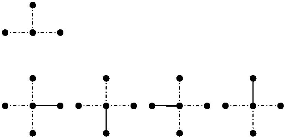
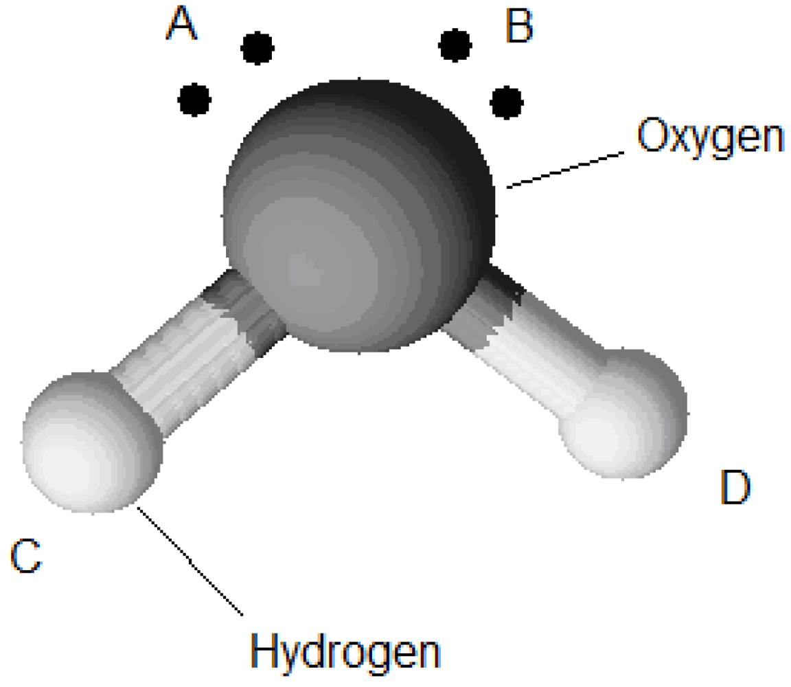
  is the association energy. The difference between the Lattice Wertheim association model and the association model used in the SAFT equation of state lies in the considerations of the quantity occurring in Equation (89) and the similar quantity, , called association volume. The association volume depends on the density and the radial distribution function. In contrast, is a constant. For example a water molecule has four association sites, one at each proton of the hydrogen and one at each lone electron pair of the oxygen (Figure 6).
 (90)
(90) (91)
(91)
3. Calculation Examples
3.1. Binary Polymer Solutions
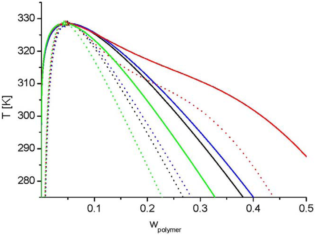
parameter in Equation (17) is expressed phenomenological as a power series of the polymer concentration. Figure 7 depicts a comparison of the modelled phase equilibrium using the FH theory and the LCT. The interaction parameter (  or ) were fitted to an arbitrarily selected critical temperature. In the FH-limit the lattice coordination number approaches infinity. In the LCT framework z can be chosen. On one side should be large in order to ensure a rapid convergence of the suggested series in 1/z. On the other hand a lower number for makes more use of the established corrections. For this reason some model calculations for different -values were performed. In Figure 7 it can be seen that a higher z-value requires a lower interaction energy for the same critical temperature. The miscibility gap gets broader, independently of the chosen z-value of the LCT. Sometimes a shoulder in the cloud point curve [83] is found experimentally. Examples are the systems polystyrene + cyclohexane and polyethylene + diphenylether [83]. This effect is often explained by polydispersity or by a complex concentration dependence of the χ-parameter. The calculation results for
  in Figure 7 show this shoulder for a monodisperse linear polymer. Therefore, the shoulder could also be discussed in terms of mixing entropy. In summary, the LCT can also be used for linear polymers, especially if complex phase diagrams are present. It is well-known that the classic Flory–Huggins theory [84,85] does not capture the effect of branching on polymer phase separation. The polymer theories which do capture the effect of branching include a scaling theory developed by Daoud et al. [65] a theory developed by Saeki [124], which replaces the standard mixing entropy term of Flory–Huggins with a combinatorial entropy term more applicable to star polymers, and the lattice cluster theory due to Freed and co-workers (e.g., [89]). All these theories predict a drop in the critical temperature and a small rise in the critical polymer concentration as a polymer becomes more branched. However, the lattice cluster theory is the most sophisticated of the three theories mentioned above.
  in a solvent occupying only one lattice site
  (solid line: binodal line, dotted line: spinodal line, stars: critical points), where the black colour depicts the results using the LCT with z = 12; ε/kB = 35 K, the blue colour those with z = 10; ε/kB = 43.86 K, the red colour those with z = 6; ε/kB = 93.62 K, and the green colour presents the results obtained by FH theory with
  .
in a solvent occupying only one lattice site (solid line: binodal line, dotted line: spinodal line, stars: critical points), where the black colour depicts the results using the LCT with z = 12; ε/kB = 35 K, the blue colour those with z = 10; ε/kB = 43.86 K, the red colour those with z = 6; ε/kB = 93.62 K, and the green colour presents the results obtained by FH theory with .
.
in a solvent occupying only one lattice site (solid line: binodal line, dotted line: spinodal line, stars: critical points), where the black colour depicts the results using the LCT with z = 12; ε/kB = 35 K, the blue colour those with z = 10; ε/kB = 43.86 K, the red colour those with z = 6; ε/kB = 93.62 K, and the green colour presents the results obtained by FH theory with . was set to 12. Details about the fitting procedure and the used data are given in the literature [54,55,56,57,58].
| Component |  |  | Ref. |
|---|---|---|---|
| Boltorn H20a 1 | 0.023 | 1,200 | [54] |
| Boltorn H20b 1 | 0.023 | 1,200 | [58] |
| Boltorn U3000 | 0.023 | 1,200 | [55] |
| Water | 0.01 | 1,800 | [54] |
| Propan-1-ol | 0.011 | 1,745 | [56] |
| Butan-1-ol | 0.01 | 1,710 | [58] |
| Component i | Component j |  |  2 2 |  | Ref. |
|---|---|---|---|---|---|
| Boltorn H20a | Water | 46.842 | 11.65 | 0.06 | [58] |
| Boltorn H20b | Water | 45.27 | 18.05 | 0.02 | [58] |
| Boltorn H20a | Propan-1-ol | 18.96 | 10.55 | 0.04 | |
| Boltorn H20b | Butan-1ol | 14.983 | 9.01 | 0.035 | [58] |
| Boltorn U3000 | Propan-1-ol | 12.59 | 3.9 | 0.03 | |
| Boltorn U3000 | Butan-1-ol | 10.54 | 2.03 | 0.02 | |
| Propan-1-ol | Water | 64 (fitted to binary VLE) 45 (fitted to ternary LLE) | [56] | ||
| Butan-1-ol | Water | 184.622 | 57.5 | 0.03 | [58] |
 -value. Like shown in Figure 7 the LCT is in principle able to describe a shoulder in the cloud point curve.
3.2. Ternary Polymer Solutions
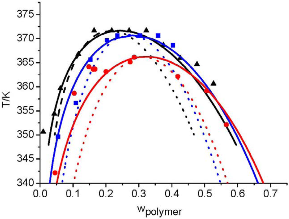
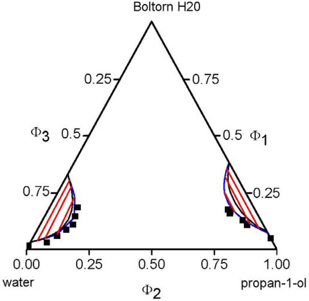
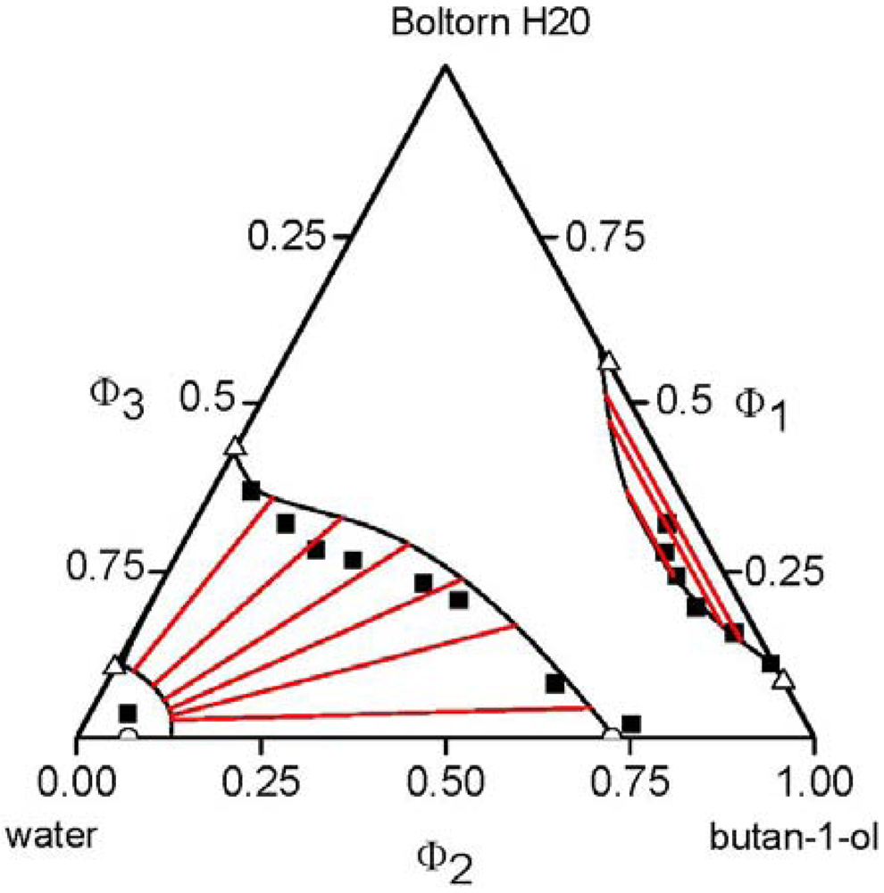
, of each component pair. For the analysis of the predictive power of the LCT, two mixtures were selected, namely Boltorn H20 + water + propan-1-ol and Boltorn H20 + water + butan-1-ol. Boltorn H20 + water as well as Boltorn + alcohol, either propan-1-ol or butan-1-ol, exhibit a LLE (Figure 8) and hence the interaction parameters for these subsystems can be estimated using the corresponding phase binary diagram [54,58]. The most important difference between these mixtures lies in the water-alcohol mixture, where water + butan-1-ol has a miscibility gap and water + propan-1-ol does not. For the ternary system Boltorn H20 + butan-1-ol + water, where all binary subsystems show a miscibility gap, all parameters can be estimated using LLE of the binary subsystems. In contrast, for the ternary Boltorn H20 + propan-1-ol + water the parameter describing the binary subsystem propan-1-ol + water must be adjusted to other thermodynamic properties. Experimentally, it was found that two separated miscibility gaps in the Gibbs triangle at constant temperature appear [56]. If the binary interaction parameter between the components of the mixed solvent is set to zero qualitative wrong phase behaviour with a miscibility gap ranged from the water-rich side to the propan-1-ol-rich side is predicted by the LCT [56]. One possibility to estimate this missing parameter is the use of VLE data for this system [56]. The VLE of the system water + propan-1-ol is characterized by an azeotropic point at atmospheric pressure. The interaction parameter was adjusted to the azeotropic temperature at atmospheric pressure, and at the same time the mole fraction at the azeotropic point is calculated exactly, because of the calculation of the activity coefficients with a high accuracy. Using this fitted parameter ∆ε23/kB = 64 K (Table 6) the experimental phase behaviour of the ternary system can be predicted quite close to the experimental data, like shown via the black lines in Figure 10. A slight readjustment of this parameter by changing its numerical value from ∆ε23/kB = 64 K to ∆ε23/kB = 45 K (Table 6) permits an excellent description of the ternary phase behaviour (blue lines in Figure 10).  .
.
.
.

3.4. Polymer Mixtures

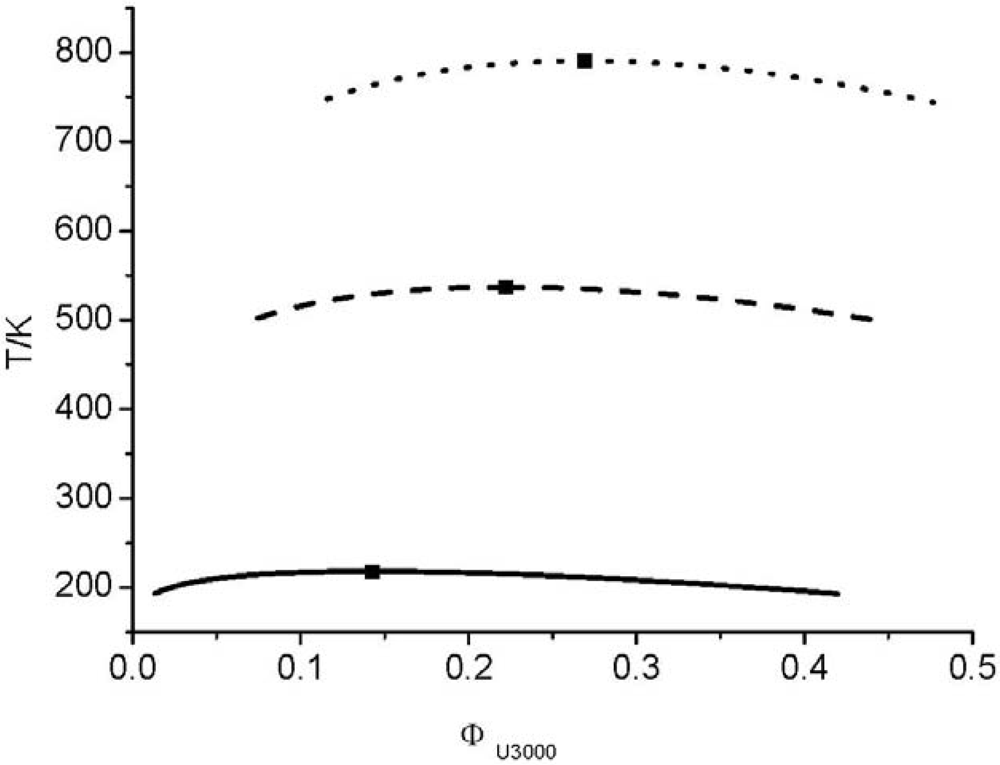
 and consequently the segment number M1) further leads to an UCST which is above the degradation temperature of the hyperbranched polymers. In other words, the LCT predicts that it is not possible to prepare a homogenous mixture made from Boltorn H40 and Boltorn U3000.
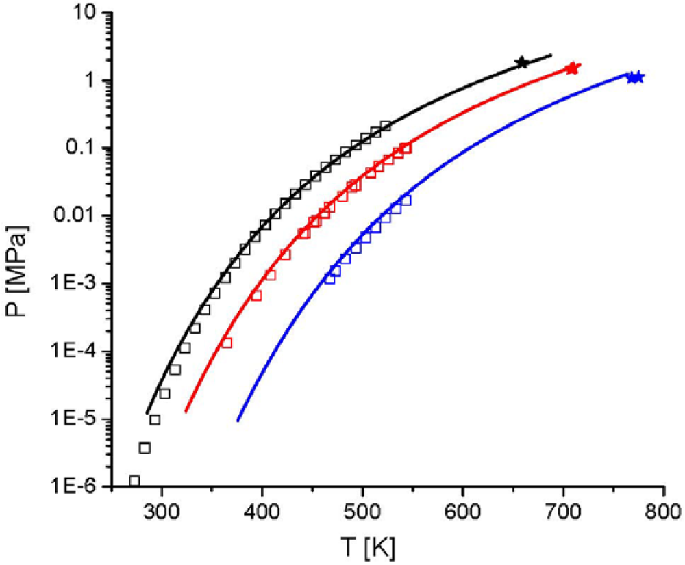
3.5. Compressible LCT
and the second one is the interaction energy, . From Figure 14 the potential of this new equation of state can be seen, because the experimental data were described with a high accuracy, although only two pure component parameters are used. 4. Summary
Acknowledgments
References
- Zou, J.; Shi, W.; Wang, J.; Bo, J. Encapsulation and controlled release of a hydrophobic drug using a novel nanoparticle forming hyperbranched polyester. Macromol. Biosci. 2005, 5, 662–668. [Google Scholar] [CrossRef]
- Paleos, C.M.; Tsiourvas, D.; Sideratou, Z.; Tziveleka, L.-A. Drug delivery using multifunctional dendrimers and hyperbranched polymers. Expert Opin. Drug Deliv. 2010, 7, 1387–1398. [Google Scholar] [CrossRef]
- Frey, H.; Haag, R. Dendritic polyglycerol: A new versatile biocompatible material. Rev. Mol. Biotechnol. 2002, 90, 257–267. [Google Scholar] [CrossRef]
- Svenson, S.; Tomalia, D.A. Dendrimers in biomedical applications—Reflections on the field. Adv. Drug Deliv. Rev. 2005, 57, 2106–2129. [Google Scholar] [CrossRef]
- Kainthan, R.K.; Gnanamani, M.; Ganguli, M.; Ghosh, T.; Brooks, D.E.; Maiti, S.; Kizhakkedathu, J.N. Blood compatibility of novel water soluble hyperbranched polyglycerol-based multivalent cationic polymers and their interaction with DNA. Biomaterials 2006, 27, 5377–5390. [Google Scholar] [CrossRef]
- Reichelt, S.; Eichhorn, K.-J.; Aulich, D.; Hinrichs, K.; Jain, N.; Appelhans, D.; Voit, B. Functionalization of solid surfaces with hyperbranched polyesters to control protein adsorption. Colloids Surfaces B 2009, 69, 169–177. [Google Scholar] [CrossRef]
- Xue, L.; Dai, S.; Li, Z. Biodegradable shape-memory block co-polymers for fast self-expandable stents. Biomaterials 2010, 31, 8132–8140. [Google Scholar] [CrossRef]
- Shepherd, J.; Sarker, P.; Rimmer, S.; Swanson, L.; MacNeil, S.; Douglas, I. Hyperbranched poly(NIPAM) polymers modified with antibiotics for the reduction of bacterial burden in infected human tissue engineered skin. Biomaterials 2011, 32, 258–267. [Google Scholar]
- Tuchbreiter, L.; Mecking, S. Hydroformylation with dendritic-polymer-stabilized rhodium colloids as catalyst precursors. Macromol. Chem. Phys. 2007, 208, 1688–1693. [Google Scholar] [CrossRef]
- Zhang, G.; Fan, X.; Kong, J.; Liu, Y.; Xie, Y. Hyperbranched organosilicon polymers. Prog. Chem. 2008, 20, 326–338. [Google Scholar]
- Marty, J.-D.; Martinez-Aripe, E.; Mingotaud, A.-F.; Mingotaud, C. Hyperbranched polyamidoamine as stabilizer for catalytically active nanoparticles in water. J. Colloid Interf. Sci. 2008, 326, 51–54. [Google Scholar]
- Tahara, K.; Shimakoshi, H.; Tanaka, A.; Hisaeda, Y. Synthesis, characterization and catalytic function of a B 12-hyperbranched polymer. Dalton Trans. 2010, 39, 3035–3042. [Google Scholar]
- Cypryk, M.; Pospiech, P.; Strzelec, K.; Wasikowska, K.; Sobczak, J.W. Soluble polysiloxane-supported palladium catalysts for the Mizoroki-Heck reaction. J. Mol. Catal. A 2010, 319, 30–38. [Google Scholar] [CrossRef]
- Yin, Y.; Yang, L.; Yoshino, M.; Fang, J.; Tanaka, K.; Kita, H.; Okamoto, K.-I. Synthesis and gas permeation properties of star-like poly(ethylene oxide)s using hyperbranched polyimide as central core. Polym. J. 2004, 36, 294–302. [Google Scholar] [CrossRef]
- Suda, T.; Yamazaki, K.; Kawakami, H. Syntheses of sulfonated star-hyperbranched polyimides and their proton exchange membrane properties. J. Power Sour. 2010, 195, 4641–4646. [Google Scholar]
- Kakimoto, M.-A.; Grunzinger, S.J.; Hayakawa, T. Hyperbranched poly(ether sulfone)s: Preparation and application to ion-exchange membranes. Polym. J. 2010, 42, 697–705. [Google Scholar] [CrossRef]
- Sterescu, D.M.; Stamatialis, D.F.; Mendes, E.; Kruse, J.; Rätzke, K.; Faupel, F.; Wessling, M. Boltom-modified poly(2,6-dimethyl-1,4-phenylene oxide) gas separation membranes. Macromolecules 2007, 40, 5400–5410. [Google Scholar]
- Wei, X.-Z.; Zhu, L.-P.; Deng, H.-Y.; Xu, Y.-Y.; Zhu, B.-K.; Huang, Z.-M. New type of nanofiltration membrane based on crosslinked hyperbranched polymers. J. Membr. Sci. 2008, 323, 278–287. [Google Scholar] [CrossRef]
- Peter, J.; Kosmala, B.; Bleha, M. Synthesis of hyperbranched copolyimides and their application as selective layers in composite membranes. Desalination 2009, 245, 516–526. [Google Scholar] [CrossRef]
- Arkas, M.; Tsiourvas, D.; Paleos, C.M. Functional dendritic polymers for the development of hybrid materials for water purification. Macromol. Mater. Eng. 2010, 295, 883–898. [Google Scholar] [CrossRef]
- Seiler, M. Hyperbranched polymers: Phase behavior and new applications in the field of chemical engineering. Fluid Phase Equilib. 2006, 241, 155–174. [Google Scholar] [CrossRef]
- Rehim, M.A.; Fahmy, H.M.; Mohamed, Z.E.; Abo-Shosha, M.H.; Ibrahim, N.A. Synthesis, characterisation and utilisation of hyperbranched poly (ester-amide) for the removal of some anionic dyestuffs from their aqueous solutions. Pigment Resin Technol. 2010, 39, 149–155. [Google Scholar]
- Chen, Y.Z.; Peng, P.; Guo, Z.X.; Yu, J.; Zhan, M.S. Effect of hyperbranched poly(ester amine) additive on electrospinning of low concentration poly(methyl methacrylate) solutions. J. Appl. Polym. Sci. 2010, 115, 3687–3696. [Google Scholar] [CrossRef]
- Seiler, M. Dendritic polymers—Interdisciplinary research and emerging applications from unique structural properties. Chem. Eng. Technol. 2002, 25, 237–253. [Google Scholar] [CrossRef]
- Feng, J.; Li, Y.; Yang, M. Hyperbranched copolymer containing triphenylamine and divinyl bipyridyl units for fluorescent chemosensors. J. Polym. Sci. Part A 2009, 47, 222–230. [Google Scholar] [CrossRef]
- Hartmann-Thompson, C.; Keeley, D.L.; Rousseau, J.R.; Dvornic, P.R. Fluorescent dendritic polymers and nanostructured coatings for the detection of chemical warfare agents and other analytes. J. Polym. Sci. Part A 2009, 47, 5101–5115. [Google Scholar]
- Liu, Y.; Dong, Y.; Jauw, J.; Linman, M.J.; Cheng, Q. Highly sensitive detection of protein toxins by surface plasmon resonance with biotinylation-based inline atom transfer radical polymerization amplification. Anal. Chem. 2010, 82, 3679–3685. [Google Scholar]
- Caminade, A.M.; Delavaux-Nicot, B.; Laurent, R.; Majoral, J.P. Sensitive sensors based on phosphorus dendrimers. Curr. Org. Chem. 2010, 14, 500–515. [Google Scholar] [CrossRef]
- Foix, D.; Erber, M.; Voit, B.; Lederer, A.; Ramis, X.; Mantecón, A.; Serra, A. New hyperbranched polyester modified DGEBA thermosets with improved chemical reworkability. Polym. Degrad. Stab. 2010, 95, 445–452. [Google Scholar] [CrossRef]
- Morell, M.; Erber, M.; Ramis, X.; Ferrando, F.; Voit, B.; Serra, A. New epoxy thermosets modified with hyperbranched poly(ester-amide) of different molecular weight. Eur. Polym. J. 2010, 46, 1498–1509. [Google Scholar] [CrossRef]
- Deka, H.; Karak, N. Bio-based hyperbranched polyurethane/clay nanocomposites: Adhesive mechanical and thermal properties. Polym. Adv. Technol. 2011, 22, 973–980. [Google Scholar] [CrossRef]
- Kim, Y.H.; Webster, O.W. Hyperbranched polyphenylenes. Macromolecules 1992, 25, 5561–5572. [Google Scholar] [CrossRef]
- Morgan, S.; Ye, Z.; Subramanian, R.; Zhu, S. Higher-molecular-weight hyperbranched polyethylenes containing crosslinking structures as lubricant viscosity-index improvers. Polym. Eng. Sci. 2010, 50, 911–918. [Google Scholar] [CrossRef]
- Frey, H.; Haag, R. Dendritic polyglycerol: A new versatile biocompatible material. Rev. Mol. Biotechnol. 2002, 90, 257–267. [Google Scholar] [CrossRef]
- Kainthan, R.K.; Gnanamani, M.; Ganguli, M.; Ghosh, T.; Brooks, D.E.; Maiti, S.; Kizhakkedathu, J.N. Blood compatibility of novel water soluble hyperbranched polyglycerol-based multivalent cationic polymers and their interaction with DNA. Biomaterials 2006, 27, 5377–5390. [Google Scholar]
- Rossi, N.A.A.; Constantinescu, I.; Kainthan, R.K.; Brooks, D.E.; Scott, M.D.; Kizhakkedathu, J.N. Red blood cell membrane grafting of multi-functional hyperbranched polyglycerols. Biomaterials 2010, 31, 4167–4178. [Google Scholar]
- Perumal, O.; Khandare, J.; Kolhe, P.; Kannan, S.; Lieh-Lai, M.; Kannan, R.M. Effects of branching architecture and linker on the activity of hyperbranched polymer-drug conjugates. Bioconjug. Chem. 2009, 20, 842–846. [Google Scholar] [CrossRef]
- Kumar, K.R.; Brooks, D.E. Comparison of hyperbranched and linear polyglycidol unimolecular reverse micelles as nanoreactors and nanocapsules. Macromol. Rapid Commun. 2005, 26, 155–159. [Google Scholar] [CrossRef]
- Wang, T.; Wu, Y.; Li, M. Novel hyperbranched poly (amine-ester)-poly (lactide-co-glycolide) polymeric micelles as amphotericin B carriers. Polym. Bull. 2010, 65, 425–442. [Google Scholar] [CrossRef]
- Kurniasih, I.N.; Liang, H.; Rabe, J.P.; Haag, R. Supramolecular aggregates of water soluble dendritic polyglycerol architectures for the solubilization of hydrophobic compounds. Macromol. Rapid Commun. 2010, 31, 1516–1520. [Google Scholar] [CrossRef]
- Oudshoorn, M.H.M.; Penterman, R.; Rissmann, R.; Bouwstra, J.A.; Broer, D.J.; Hennink, W.E. Preparation and characterization of structured hydrogel microparticles based on cross-linked hyperbranched polyglycerol. Langmuir 2007, 23, 11819–11825. [Google Scholar]
- Höbel, S.; Loos, A.; Appelhans, D.; Schwarz, S.; Seidel, J.; Voit, B.; Aigner, A. Maltose- and maltotriose-modified, hyperbranched poly(ethylene imine)s (OM_PEIs): Physicochemical and biological properties of DNA and siRNA complexes. J. Control. Release 2011, 149, 146–158. [Google Scholar] [CrossRef]
- Zhao, D.; Gong, T.; Zhu, D.; Zhang, Z.; Sun, X. Comprehensive comparison of two new biodegradable gene carriers. Int. J. Pharm. 2011, 413, 260–270. [Google Scholar] [CrossRef]
- Wang, J.; Xu, T. Facile construction of multivalent targeted drug delivery system from Boltorn® series hyperbranched aliphatic polyester and folic acid. Polym. Adv. Technol. 2011, 22, 763–767. [Google Scholar] [CrossRef]
- Jain, N.K.; Gupta, U. Application of dendrimer-drug complexation in the enhancement of drug solubility and bioavailability. Expert Opin. Drug Metab. Toxicol. 2008, 4, 1035–1052. [Google Scholar] [CrossRef]
- Paleos, C.M.; Tsiourvas, D.; Sideratou, Z.; Tziveleka, L.A. Drug delivery using multifunctional dendrimers and hyperbranched polymers. Expert Opin. Drug Deliv. 2010, 7, 1387–1398. [Google Scholar] [CrossRef]
- Kim, W.J.; Bonoiu, A.C.; Hayakawa, T.; Xia, C.; Kakimoto, M.A.; Pudavar, H.E.; Lee, K.S.; Prasad, P.N. Hyperbranched polysiloxysilane nanoparticles: Surface charge control of nonviral gene delivery vectors and nanoprobes. Int. J. Pharm. 2009, 376, 141–52. [Google Scholar] [CrossRef]
- Astruc, D.; Boisselier, E.; Ornelas, C. Dendrimers designed for functions: From physical, photophysical, and supramolecular properties to applications in sensing, catalysis, molecular electronics, photonics, and nanomedicine. Chem. Rev. 2010, 110, 1857–1959. [Google Scholar] [CrossRef]
- Irfan, M.; Seiler, M. Encapsulation using hyperbranched polymers: From research and technologies to emerging applications. Ind. Eng. Chem. Res. 2010, 49, 1169–1196. [Google Scholar] [CrossRef]
- Wilms, D.; Stiriba, S.E.; Frey, H. Hyperbranched polyglycerols: From the controlled synthesis of biocompatible polyether polyols to multipurpose applications. Acc. Chem. Res. 2010, 43, 129–141. [Google Scholar] [CrossRef]
- Wurm, F.; Frey, H. Linear-dendritic block copolymers: The state of the art and exciting perspectives. Prog. Polym. Sci. 2011, 36, 1–52. [Google Scholar] [CrossRef]
- Zagar, E.; Zigon, M. Aliphatic hyperbranched polyesters based on 2,2-bis(methylol)propionic acid - Determination of structure, solution and bulk properties. Prog. Polym. Sci. 2011, 36, 53–88. [Google Scholar] [CrossRef]
- Zeiner, T.; Browarzik, D.; Enders, S. Calculation of the liquid-liquid equilibrium of aqueous solutions of hyperbranched polymers. Fluid Phase Equilib. 2009, 286, 127–133. [Google Scholar] [CrossRef]
- Zeiner, T.; Schrader, P.; Enders, S.; Browarzik, D. Phase- and interfacial behavior of hyperbranched polymer solutions. Fluid Phase Equilib. 2011, 302, 321–330. [Google Scholar] [CrossRef]
- Enders, S.; Zeiner, T. Application of Lattice Cluster Theory to the Calculation of Miscibility—and Interfacial Behavior of Polymer Containing Systems. In Polymer Phase Behavior; Ehlers, T.P., Wilhelm, J.K., Eds.; Nova Science Publishers, Inc.: Hauppauge, NY, USA, 2011. [Google Scholar]
- Zeiner, T.; Enders, S. Phase-behavior of hyperbranched polymer solutions in mixed solvents. Chem. Eng. Sci. 2011, 66, 5244–5252. [Google Scholar] [CrossRef]
- Zeiner, T.; Browarzik, C.; Browarzik, D.; Enders, S. Calculation of the liquid-liquid equilibrium of solutions of hyperbranched polymers with the lattice-cluster theory combined with an association model. J. Chem. Thermodyn. 2011, 43, 1969–1976. [Google Scholar] [CrossRef]
- Zeiner, T.; Puyan, M.J.; Schrader, P.; Browarzik, C.; Enders, S. Phase behavior of hyperbranched polymer in demixed solvent. Mol. Phys. 2012, in press. [Google Scholar]
- Kleintjens, L.A.; Schoffeleers, H.M.; Koningsveld, R. Entmischung in hochmolekularen Vielstoffsystemen, XVII. Eine Wechselwirkungsfunktion für Lösungen verzweigter Polymerer. Berichte der Bunsengesellschaft für physikalische Chemie 1977, 81, 980–985. [Google Scholar]
- de Loos, T.W.; Poot, W.; Lichtenthaler, R.N. The influence of branching on high-pressure vapor-liquid equilibria in systems of ethylene and polyethylene. J. Supercrit Fluids 1995, 8, 282–286. [Google Scholar] [CrossRef]
- Eckelt, J.; Samadi, F.; Wurm, F.; Frey, H.; Wolf, B.A. Branched versus linear polyisoprene: Flory-Huggins interaction parameters for this solutions in cyclohexane. Macromol. Chem. Phys. 2009, 210, 1433–1439. [Google Scholar] [CrossRef]
- Stockmayer, W.H. Theory of molecular size distribution and gel formation in branched-chain polymers. J. Chem. Phys. 1943, 11, 45–55. [Google Scholar] [CrossRef]
- Granath, K.A. Solution properties of branched dextrans. J. Coll. Sci. 1958, 13, 308–328. [Google Scholar] [CrossRef]
- Kleintjens, L.A.; Koningsveld, R. Liquid-liquid phase separation in multicomponent polymer systems. 18. Effect of short-chain branching. Macromolecules 1980, 13, 303–310. [Google Scholar] [CrossRef]
- Daoud, M.; Pincus, P.; Stockmayer, W.H.; Witten, T. Phase separation in branched polymer solutions. Macromolecules 1983, 16, 1833–1839. [Google Scholar] [CrossRef]
- de Gennes, P.G.; Hervet, H. Statistics of starburst polymers. J. Phys. Lett. 1983, 44, 351–358. [Google Scholar] [CrossRef]
- van Hunsel, J.; Balazs, A.C.; Koningsveld, R.; MacKnight, W.J. Effect of sequence distribution on the critical composition difference in copolymer blends. Macromolecules 1988, 21, 1528–1530. [Google Scholar] [CrossRef]
- Seiler, M. Phase Behavior and New Applications of Hyperbranched Polymers in the Field of Chemical Engineering; VDI Verlag: Düsseldorf, Germany, 2004. [Google Scholar]
- Kouskoumvekaki, I.A.; Giesen, R.; Michelsen, M.L.; Kontogeorgis, G.M. Free-volume activity coefficient models for dendrimer solutions. Ind. Eng. Chem. Res. 2002, 41, 4848–4853. [Google Scholar] [CrossRef]
- Oishi, T.; Prausnitz, J.M. Estimation of solvent activities in polymer solutions using a group-contribution method. Ind. Eng. Chem. Proc. Des. Dev. 1978, 17, 333–339. [Google Scholar] [CrossRef]
- Fredenslund, A. Vapor-Liquid Equilibria Using UNIFAC, a Group-Contribution Method; Elsevier: Amsterdam, The Netherlands, 1977. [Google Scholar]
- Müller, E.A.; Gubbins, K.E. Molecular-based equations of state for associating fluids: A review of SAFT and related approaches. Ind. Eng. Chem. Res. 2001, 40, 2193–2211. [Google Scholar] [CrossRef]
- Wertheim, M.S. Fluids with highly directional attractive forces. I. Statistical thermodynamics. J. Stat. Phys. 1984, 35, 19–34. [Google Scholar] [CrossRef]
- Wertheim, M.S. Fluids with highly directional attractive forces. II. Thermodynamic perturbation theory and integral equations. J. Stat. Phys. 1984, 35, 35–47. [Google Scholar] [CrossRef]
- Wertheim, M.S. Fluids with highly directional attractive forces. III. Multiple attraction sites. J. Stat. Phys. 1986, 42, 459–476. [Google Scholar] [CrossRef]
- Wertheim, M.S. Fluids with highly directional attractive forces. IV. Equilibrium polymerization. J. Stat. Phys. 1986, 42, 477–492. [Google Scholar] [CrossRef]
- Chapman, W.G.; Gubbins, K.E.; Joslin, C.G.; Gray, C.G. Theory and simulation of associating liquid mixtures. Fluid Phase Equilib. 1986, 29, 337–346. [Google Scholar] [CrossRef]
- Gross, J.; Sadowski, G. Perturbed-chain SAFT: An equation of state based on a perturbation theory for chain molecules. Ind. Eng. Chem. Res. 2001, 40, 1244–1260. [Google Scholar] [CrossRef]
- Kozłowska, M.K.; Jürgens, B.F.; Schacht, C.S.; Gross, J.; de Loos, T.W. Phase behavior of hyperbranched polymer systems: Experiments and application of the perturbed-chain polar SAFT equation of state. J. Phys. Chem. B 2009, 113, 1022–1029. [Google Scholar]
- Blas, F.J.; Vega, L.F. Thermodynamic properties and phase equilibria of branched chain fluids using first- and second-order Wertheim’s thermodynamic perturbation theory. J. Chem. Phys. 2001. [Google Scholar] [CrossRef]
- Tompa, H. Polymer Solutions; Butterworth: London, UK, 1956. [Google Scholar]
- Kamide, K. Thermodynamics of Polymer Solutions; Elsevier: Amsterdam, The Netherlands, 1990. [Google Scholar]
- Koningsveld, R.; Stockmayer, W.H.; Nies, E. Polymer Phase Diagrams; Oxford University Press: Oxford, UK, 2001. [Google Scholar]
- Flory, P.J. Principles of Polymer Chemistry; Cornell University Press: Ithaca, NY, USA, 1953. [Google Scholar]
- Huggins, M.L. Theory of solutions of high polymers. J. Am. Chem. Soc. 1942, 64, 1712–1719. [Google Scholar] [CrossRef]
- Huggins, M.L. Physical Chemistry of High Polymers; Cornell University Press: Ithaca, NY, USA, 1953. [Google Scholar]
- Nemirovsky, A.M.; Bawendi, M.G.; Freed, K.F. attice models of polymer solutions: Monomers occupying several lattice sites. J. Chem. Phys. 1987. [Google Scholar] [CrossRef]
- Freed, K.F.; Bawendi, M.G. Lattice theories of polymeric fluids. J. Phys. Chem. 1989, 93, 2194–2203. [Google Scholar] [CrossRef]
- Dudowicz, J.; Freed, K.F. Effect of monomer structure and compressibility on the properties of multi-component polymer blends and solutions: 1. Lattice cluster theory of compressible systems. Macromolecules 1991, 24, 5076–5095. [Google Scholar] [CrossRef]
- Dudowicz, J.; Freed, M.S.; Freed, K.F. Effect of monomer structure and compressibility on the properties of multi-component polymer blends and solutions. 2. Application to binary blends. Macromolecules 1991, 24, 5096–5111. [Google Scholar] [CrossRef]
- Dudowicz, J.; Freed, K.F. Effect of monomer structure and compressibility on the properties of multi-component polymer blends and solutions. 3. Application to deuterated polystyrene [PS(D)]poly(vinyl methyl ether) (PVME) blends. Macromolecules 1991, 24, 5112–5123. [Google Scholar] [CrossRef]
- Dudowicz, J.; Freed, K.F.; Madden, W.G. Role of molecular structure on the thermodynamic properties of melts, blends, and concentrated polymer solutions: Comparison of Monte Carlo simulations with the cluster theory for the lattice model. Macromolecules 1990, 23, 4803–4819. [Google Scholar] [CrossRef]
- Jang, J.G.; Bae, Y.C. Phase behaviors of hyperbranched polymer solutions. Polymer 1999, 40, 6761–6768. [Google Scholar] [CrossRef]
- Jang, J.G.; Bae, Y.C. Phase behavior of hyperbranched polymer solutions with specific interactions. J. Chem. Phys. 2001. [Google Scholar] [CrossRef]
- Yang, J.; Peng, C.; Liu, H.; Hu, Y.; Jiang, J. A generic molecular thermodynamics model for linear and branched polymer solutions in a lattice. Fluid Phase Equilib. 2006, 244, 188–192. [Google Scholar] [CrossRef]
- Hu, Y.; Ying, X.; Wu, D.T.; Prausnitz, J.M. Molecular thermodynamics of polymer solutions. Fluid Phase Equilib. 1993, 83, 289–300. [Google Scholar] [CrossRef]
- Newkome, G.R.; Moorefield, C.N. Stiff Dendritic Macromolecules Based on Phenylacetylenes. In Advances in Dendritic Macromolecules; Newkome, G.R., Ed.; JAI Press: Greenwich, CT, USA, 1994; Volume 1, pp. 1–23. [Google Scholar]
- Economou, I.G.; Donohue, M.D. Chemical, quasi-chemical and perturbation theories for associating fluids. AIChE J. 1991, 37, 1875–1894. [Google Scholar] [CrossRef]
- Mayer, J.E.; Mayer, M.G. Statistical Mechanics; John Wiley & Sons Inc.: Hoboken, NJ, USA, 1940. [Google Scholar]
- Constantine, T. Thermodynamic analysis of the mutual solubilities of normal alkanes and water. Fluid Phase Equilib. 1999, 156, 21–33. [Google Scholar] [CrossRef]
- Schnell, M.; Stryuk, S.; Wolf, B.A. Liquid/Liquid demixing in the system n-hexane/narrowly distributed linear polyethylene. Ind. Eng. Chem. Res. 2004, 43, 2852–2859. [Google Scholar]
- Gibbs, J.W. The Collected Works of J. Willard Gibbs; Yale University Press: New Haven, CT, USA, 1957. [Google Scholar]
- Reed, T.M.; Gubbins, K.E. Applied Statistical Mechanics; McGraw-Hill Inc.: New York, NY, USA, 1973. [Google Scholar]
- Jones, G.H.; Pfeffer, W.; Raoult, F.M.; van’t Hoff, J.H.; Arrhenius, S. The Modern Theory of Solution: Memoirs by Pfeffer, van’t Hoff, Arrhenius, and Raoult; Harper: New York, NY, USA, London, UK, 1899. [Google Scholar]
- Freed, K.F. New lattice model for interacting, avoiding polymers with controlled length distribution. J. Phys. A 1985, 18, 871–877. [Google Scholar]
- de Gennes, P.G. Exponents for the excluded volume problem as derived by the Wilson method. Phys. Lett. A 1972, 38, 339–340. [Google Scholar] [CrossRef]
- des Cloizeaux, J. The Lagrangian theory of polymer solutions at intermediate concentrations. J. Phys. 1975, 36, 281–291. [Google Scholar] [CrossRef]
- Pesci, A.I.; Freed, K.F. Lattice models of polymer fluids: Monomers occupying several lattice sites. J. Chem. Phys. 1989, 90, 2003–2016. [Google Scholar] [CrossRef]
- Freed, K.F.; Dudowicz, J. Influence of monomer molecular structure on the miscibility of polymer blends. Adv. Polym. Sci. 2005, 183, 63–126. [Google Scholar] [CrossRef]
- Dudowicz, J.; Freed, K.F.; Douglas, J.F. Modification of the phase stability of polymer blends by diblock coplymer additives. Macromolecules 1995, 28, 2276–2287. [Google Scholar] [CrossRef]
- Langenbach, K. Application of Lattice Cluster Theory to Compressible Systems. Ph.D. thesis, TU Berlin, Berlin, Germany.
- Langenbach, K.; Enders, S. Development of an EOS based on lattice cluster theory. Fluid Phase Eqilib. to be submitted for publication.
- Nemirovsky, A.M.; Dudowicz, J.; Freed, K.F. Dense self-interacting lattice trees with specified topologies: From light to dense branching. Phys. Rev. A 1992, 45, 7111–7127. [Google Scholar]
- Žagar, E.; Grdadolnik, J. An infrared spectroscopic study of H-bond network in hyperbranched polyester polyol. J. Mol. Struct. 2003, 658, 143–152. [Google Scholar] [CrossRef]
- Turky, G.; Shaaban, S.S.; Schöenhals, A. Broadband dielectric spectroscopy on the molecular dynamics in different generations of hyperbranched polyester. J. Appl. Polym. Sci. 2009, 113, 2477–2484. [Google Scholar] [CrossRef]
- Tanis, I.; Karatasos, K. Local dynamics and hydrogen bonding in hyperbranched aliphatic polyesters. Macromolecules 2009, 42, 9581–9591. [Google Scholar] [CrossRef]
- Morita, T.; Hiroike, K. A new approach to the theory of classical fluids. III. Prog. Theor. Phys. 1961, 25, 537–578. [Google Scholar] [CrossRef]
- Stell, G. Cluster Expansions for Classical Systems in Equilibrium. In The Equilibrium Theory of Classical Fluids; Frisch, H.L., Lebowitz, J.L., Eds.; Frontiers in Physics; W. A. Benjamin: New York, NY, USA, 1964. [Google Scholar]
- Kirkwood, J.G.; Buff, F.P. The statistical mechanical theory of solutions. I. J. Chem. Phys. 1951. [Google Scholar] [CrossRef]
- Nies, E.; Li, T.; Berghmans, H.; Heenan, R.K.; King, S.M. Upper critical solution temperature phase behavior, composition fluctuations, and complex formation in poly (Vinyl methyl ether)/D2O solutions: Small-Angle neutron-scattering experiments and wertheim lattice thermodynamic perturbation theory predictions. J. Phys. Chem. B 2006, 110, 5321–5329. [Google Scholar]
- Nies, E.; Ramzi, A.; Berghmans, H.; Li, T.; Heenan, R.K.; King, S.M. Composition fluctuations, phase behavior, and complex formation in poly(vinyl methyl ether)/D2O investigated by small-angle neutron scattering. Macromolecules 2005, 38, 915–924. [Google Scholar]
- Langenbach, K.; Enders, S. Cross-Association of Multicomponent Systems. In Process Engineering and Chemical Plant Design; Wozny, G., Hady, L., Eds.; Universitätsverlag der TU Berlin: Berlin, Germany, 2011. [Google Scholar]
- Grenner, A.; Kontogeorgis, G.M.; von Solms, N.; Michelsen, M.L. Application of PC-SAFT to glycol containing systems—PC-SAFT towards a predictive approach. Fluid Phase Equilib. 2007, 261, 248–257. [Google Scholar] [CrossRef]
- Saeki, S. Combinatory entropy in complex polymer solutions. Polymer 2000, 41, 8331–8338. [Google Scholar] [CrossRef]
- Arya, G.; A.Z. Panagiotopoulos, A.Z. Impact of branching on the phase behavior of polymers. Macromolecules 2005, 38, 10596–10604. [Google Scholar] [CrossRef]
- Alessi, M.L.; Bittner, K.C.; Greer, S.C. Eight-arm star polystyrene in methylcyclohexane: Cloud-point curves. J. Polym. Sci. Part B 2004, 42, 129–145. [Google Scholar] [CrossRef]
- Yokoyama, H.; Takano, A.; Okado, M.; Nose, T. Phase diagram of star-shaped polystyrene/cyclohexane system: Location of critical point and profile of coexistence curve. Polymer 1991, 32, 3218–3224. [Google Scholar] [CrossRef]
- Domańska, U.; Paduszyński, K.; ZoŁek-Tryznowska, Z. Liquid-liquid phase equilibria of binary systems containing hyperbranched polymer B-U3000: Experimental study and modeling in terms of lattice cluster theory. J. Chem. Eng. Data 2010, 55, 3842–3846. [Google Scholar] [CrossRef]
- Stephenson, R.; Stuart, J. Mutual binary solubilities: Water-alcohols and water-esters. J. Chem. Eng. Data 1986, 31, 56–70. [Google Scholar] [CrossRef]
- Samadi, F.; Eckelt, J.; Wolf, B.A.; Lopez-Villanueva, F.J.; Frey, H. Branched versus linear polyisoprene: Fractionation and phase behavior. Eur. Polym. J. 2007, 43, 4236–4243. [Google Scholar] [CrossRef]
- Francis, A.W. Pressure-temperature-liquid density relations of pure hydrocarbons. Ind. Eng. Chem. 1957, 49, 1779–1786. [Google Scholar] [CrossRef]
- Vargaftik, N.B. Tables on the Thermophysical Properties of Liquids and Gases; Hemisphere Publishing Corporation: Washington, DC, USA, 1975. [Google Scholar]
- Green, D.W.; Perry, R.H. Perry’s Chemical Engineers’ Handbook; McGraw-Hill Professional: New York, NY, USA, 1997. [Google Scholar]
- Stull, D.R. Vapor pressure of pure substances. Organic and inorganic compounds. Ind. Eng. Chem. 1947, 39, 517–540. [Google Scholar] [CrossRef]
- Camin, D.L.; Rossini, F.D. Physical properties of fourteen API research hydrocarbons, C9 to C15. J. Phys. Chem. 1955, 59, 1173–1179. [Google Scholar] [CrossRef]
- Ambrose, D.; Tsonopoulos, C. Vapor-liquid critical properties of elements and compounds. 2. Normal Alkanes. J. Chem. Eng. Data 1995, 40, 531–546. [Google Scholar] [CrossRef]
© 2012 by the authors; licensee MDPI, Basel, Switzerland. This article is an open-access article distributed under the terms and conditions of the Creative Commons Attribution license (http://creativecommons.org/licenses/by/3.0/).
Share and Cite
Enders, S.; Langenbach, K.; Schrader, P.; Zeiner, T. Phase Diagrams for Systems Containing Hyperbranched Polymers. Polymers 2012, 4, 72-115. https://doi.org/10.3390/polym4010072
Enders S, Langenbach K, Schrader P, Zeiner T. Phase Diagrams for Systems Containing Hyperbranched Polymers. Polymers. 2012; 4(1):72-115. https://doi.org/10.3390/polym4010072
Chicago/Turabian StyleEnders, Sabine, Kai Langenbach, Philipp Schrader, and Tim Zeiner. 2012. "Phase Diagrams for Systems Containing Hyperbranched Polymers" Polymers 4, no. 1: 72-115. https://doi.org/10.3390/polym4010072