Extraction of the Polyurethane Layer in Textile Composites for Textronics Applications Using Optical Coherence Tomography

 , ,
, ,
Abstract
:1. Introduction
2. Material and Methods
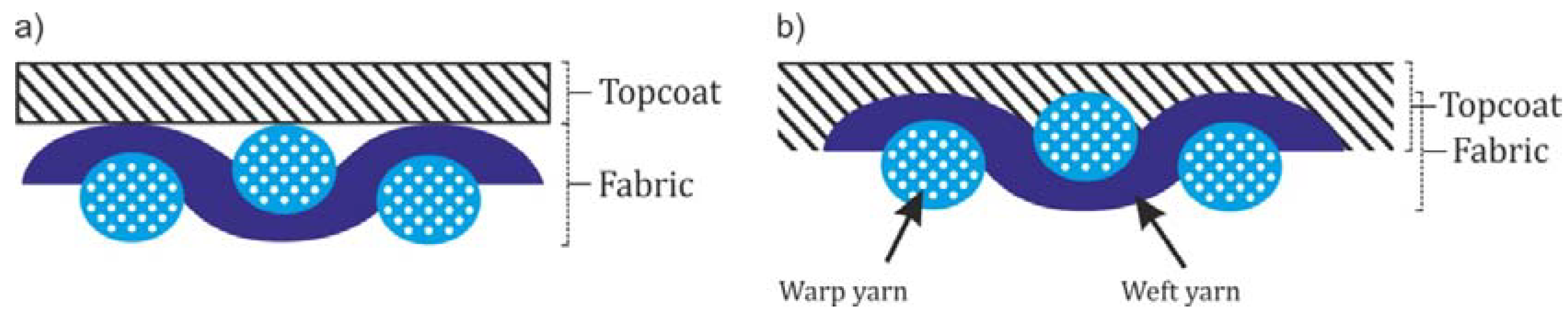
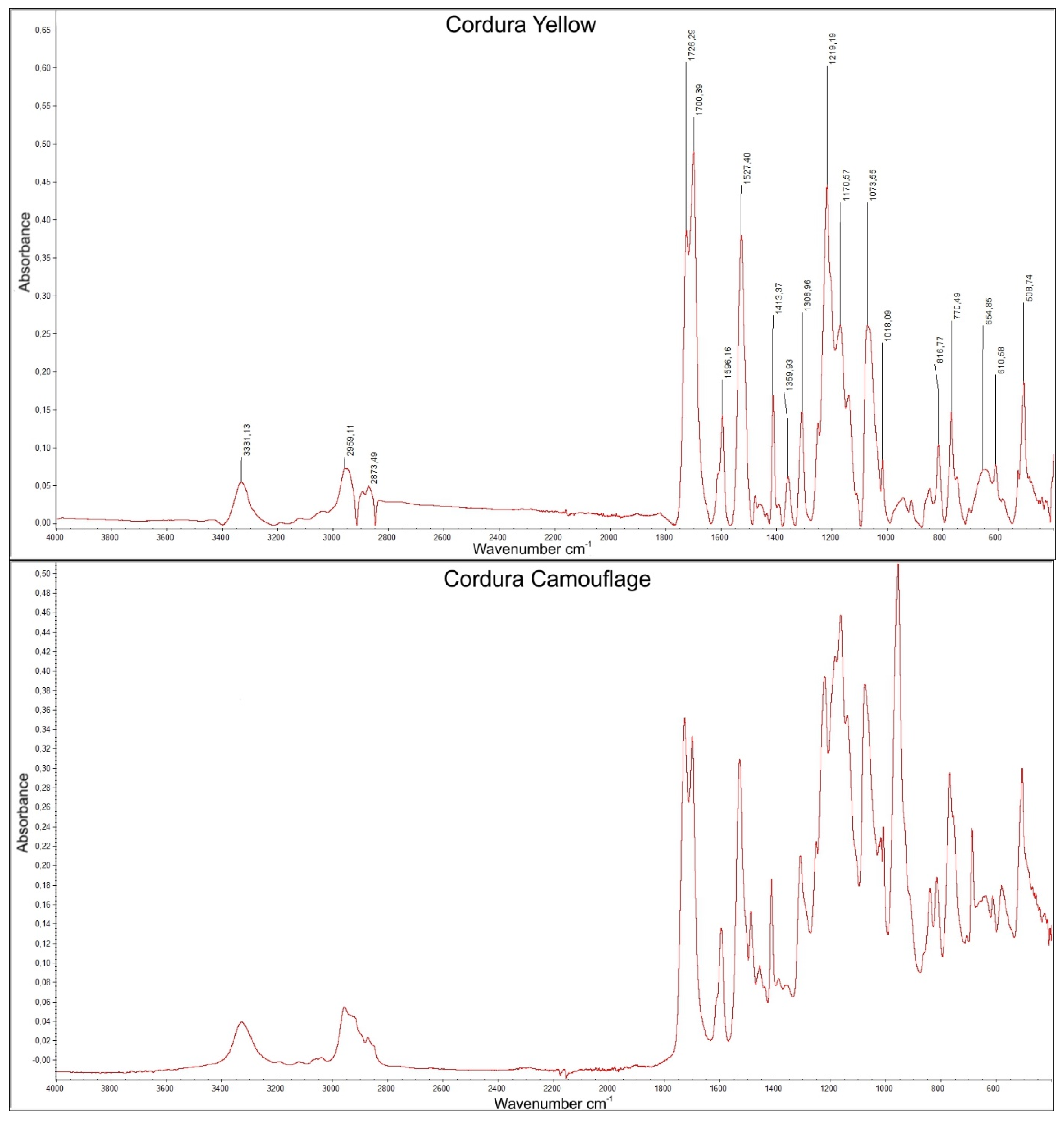
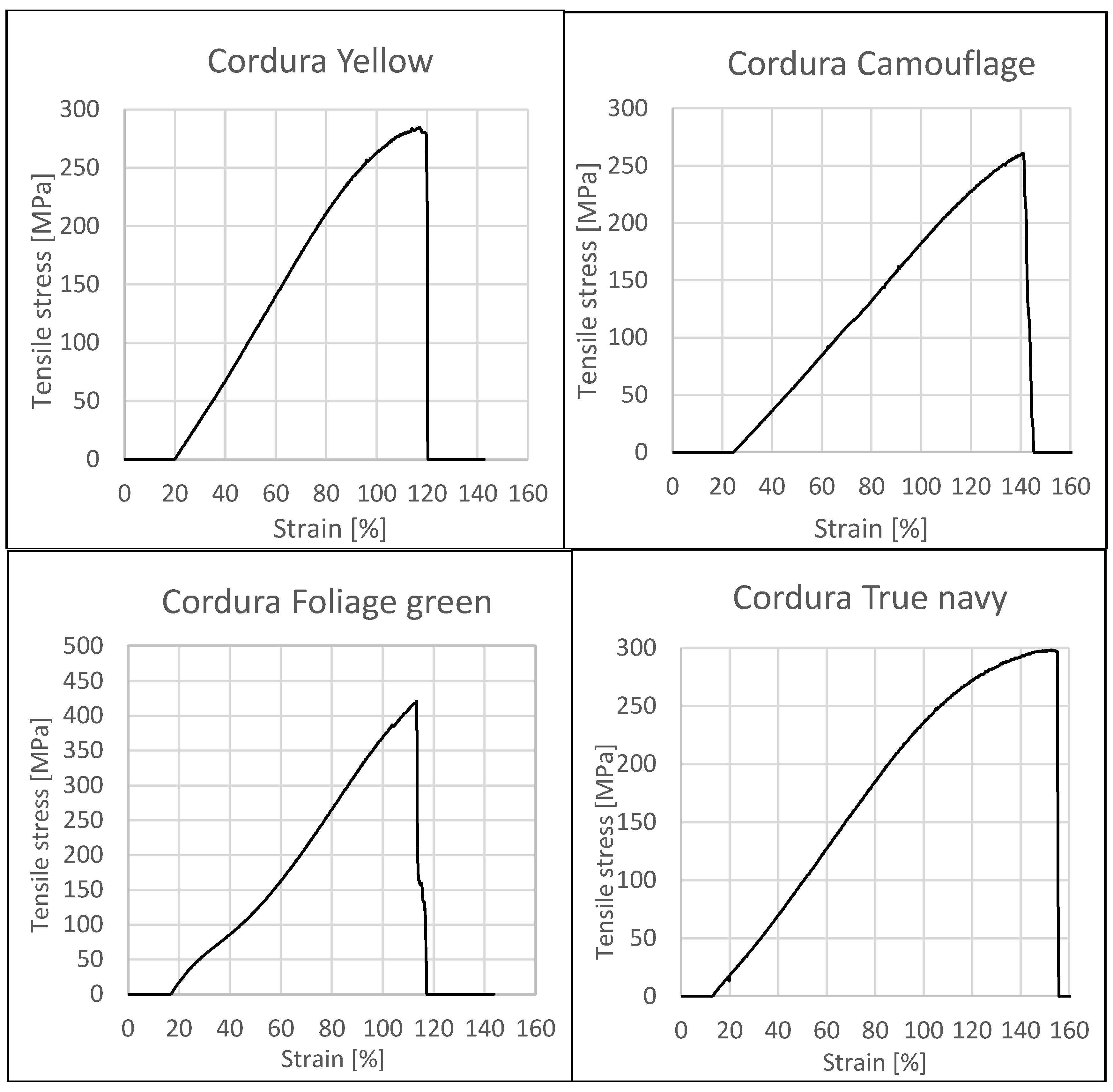
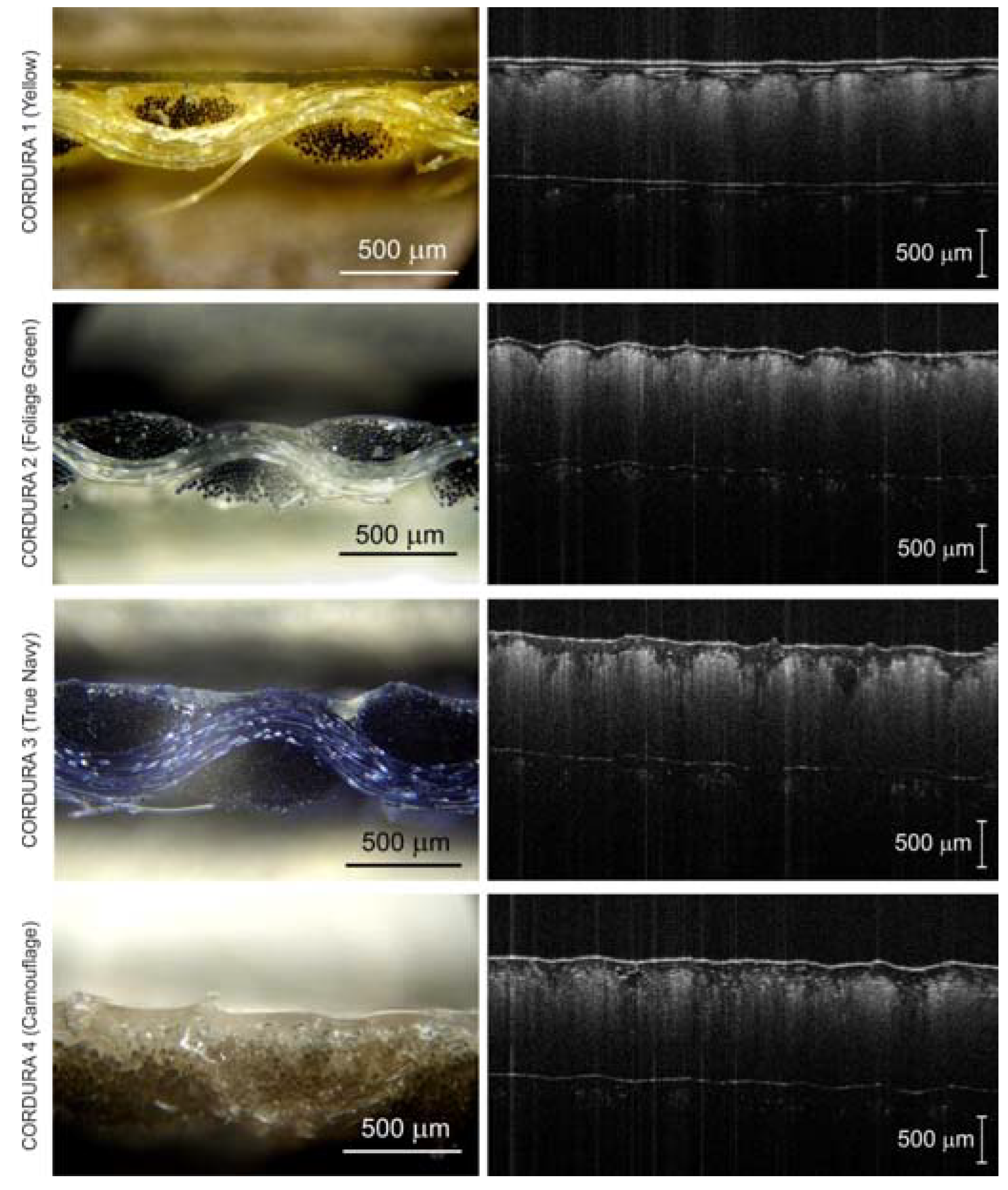
2.1. Cordura Samples
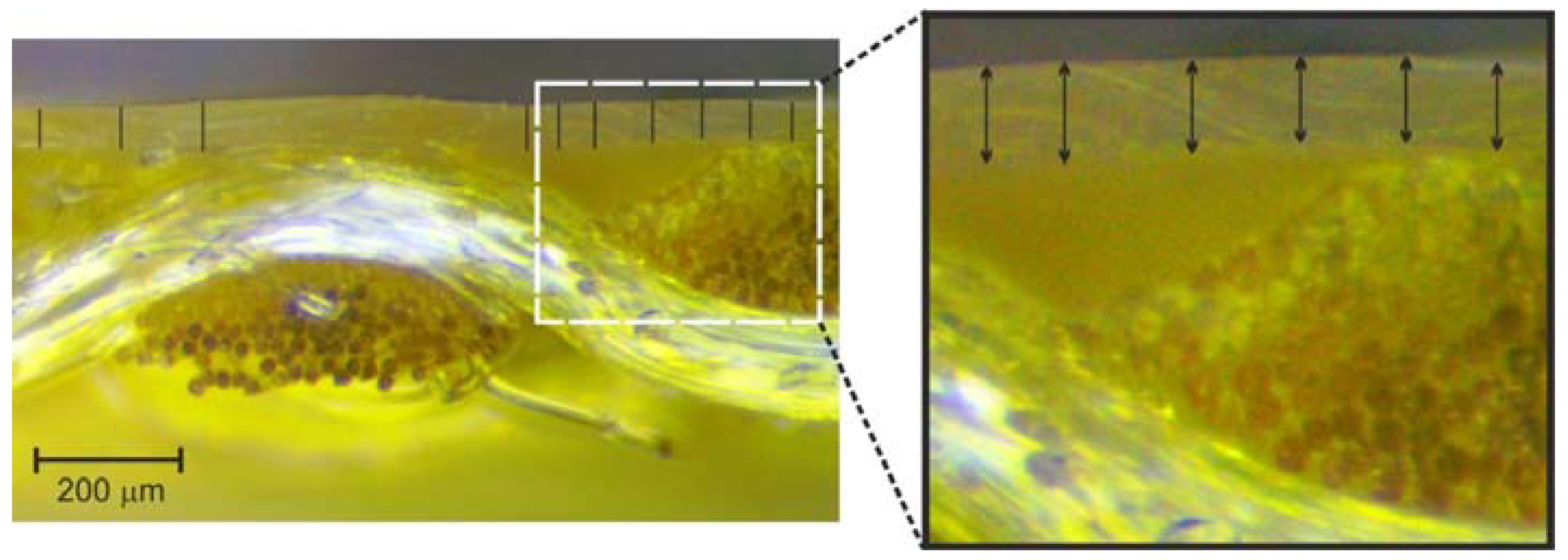
2.2. Measurement with Microscope Images
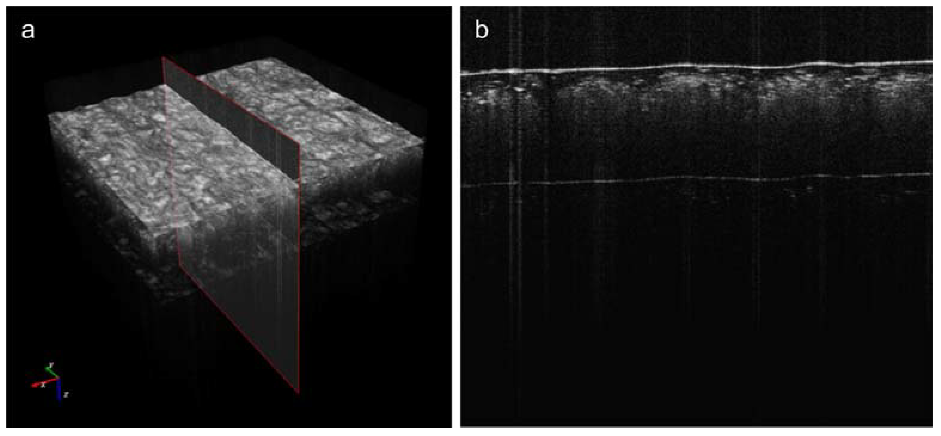
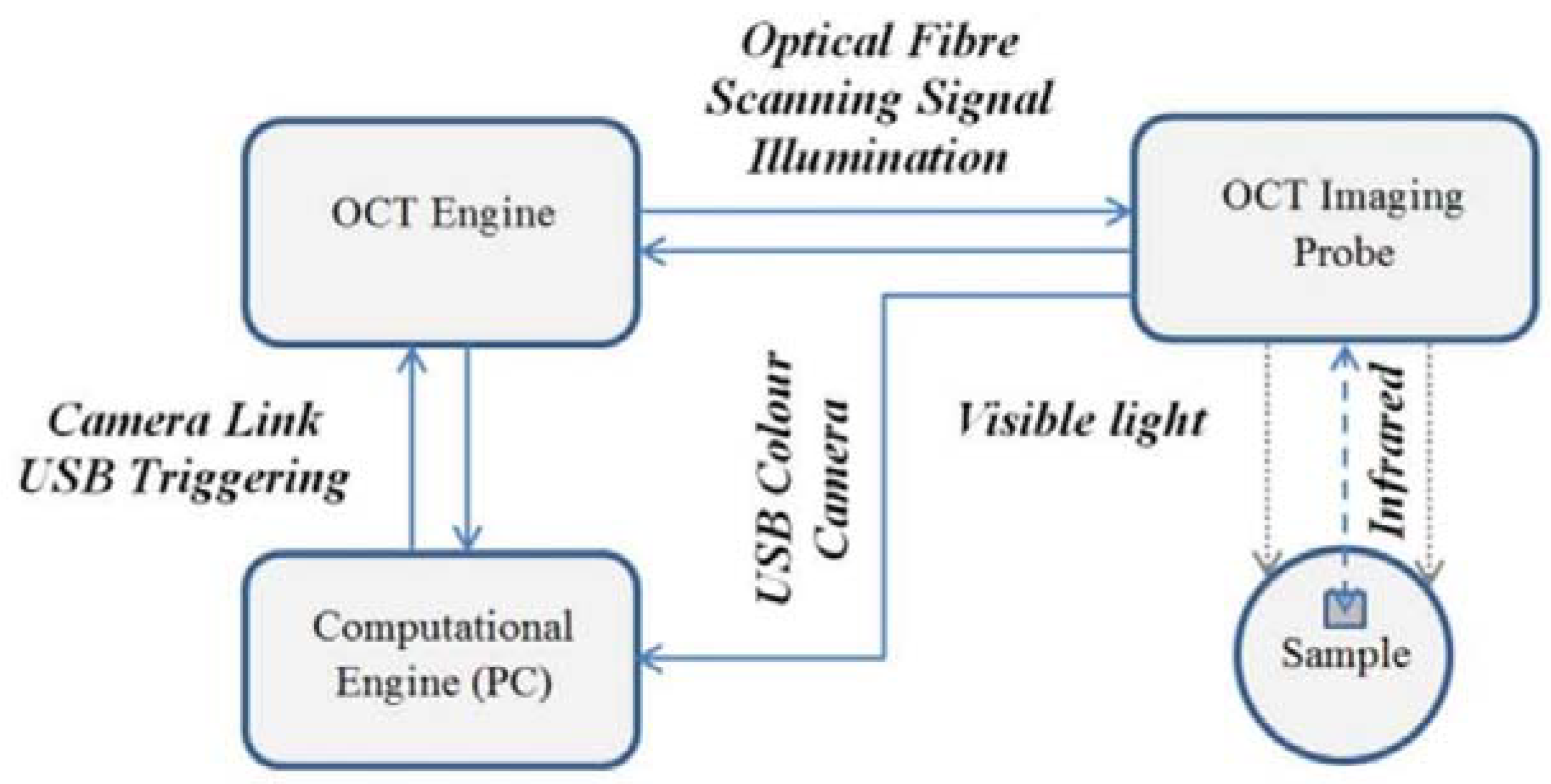
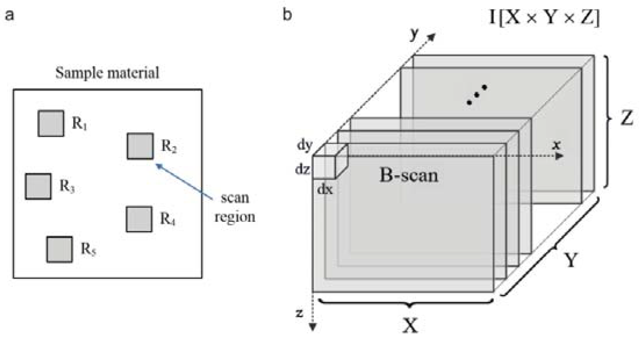
2.3. Acquisition of OCT Images
2.4. Computing Environment
3. Image Analysis
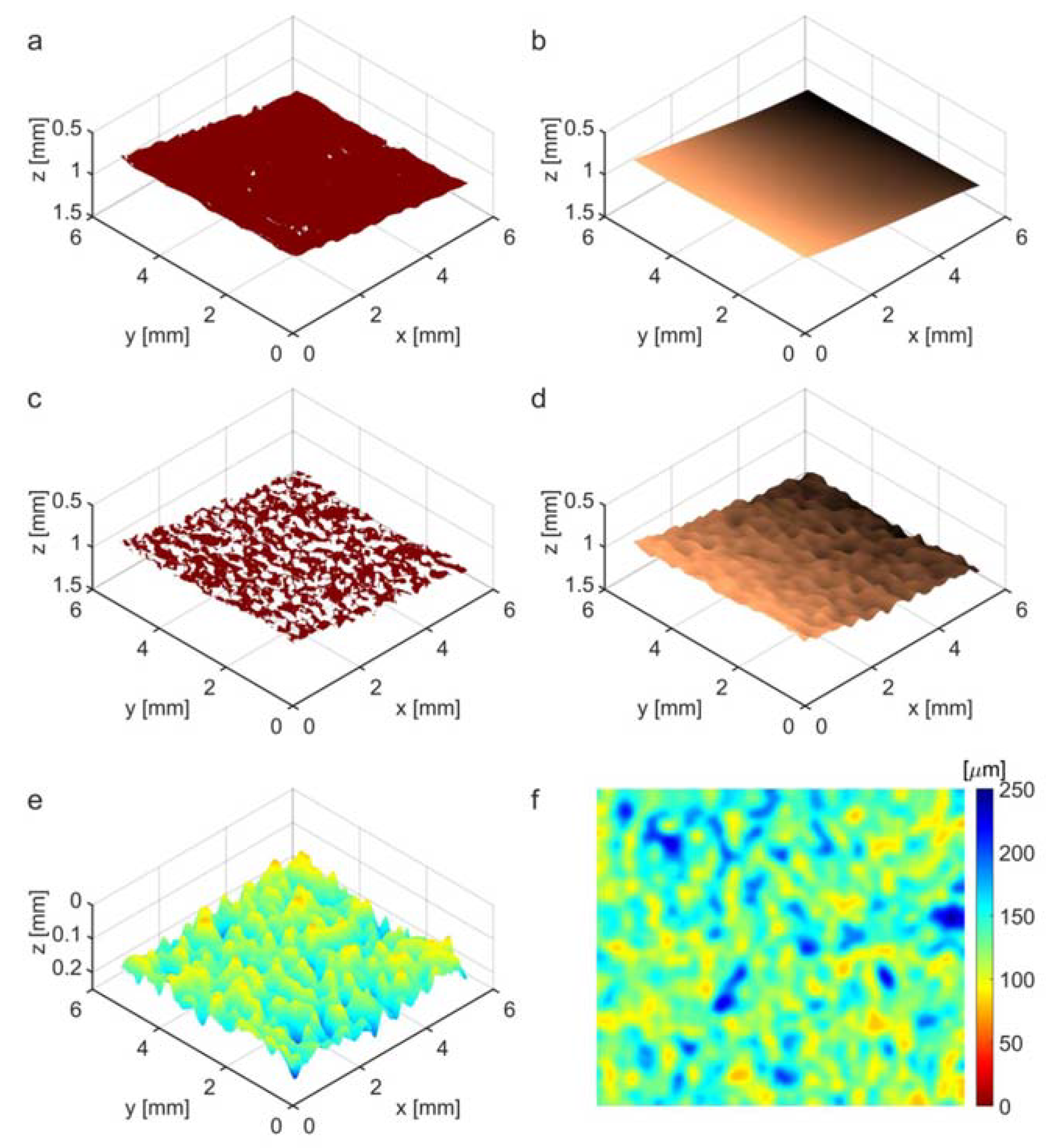
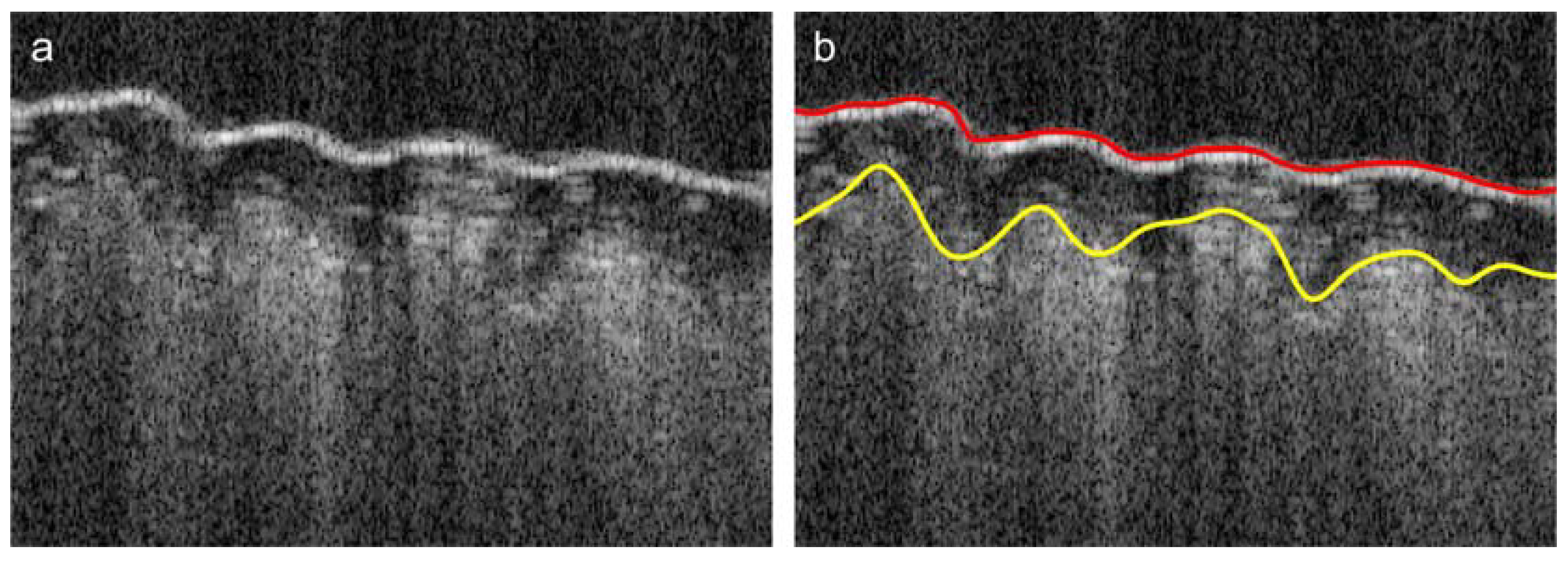
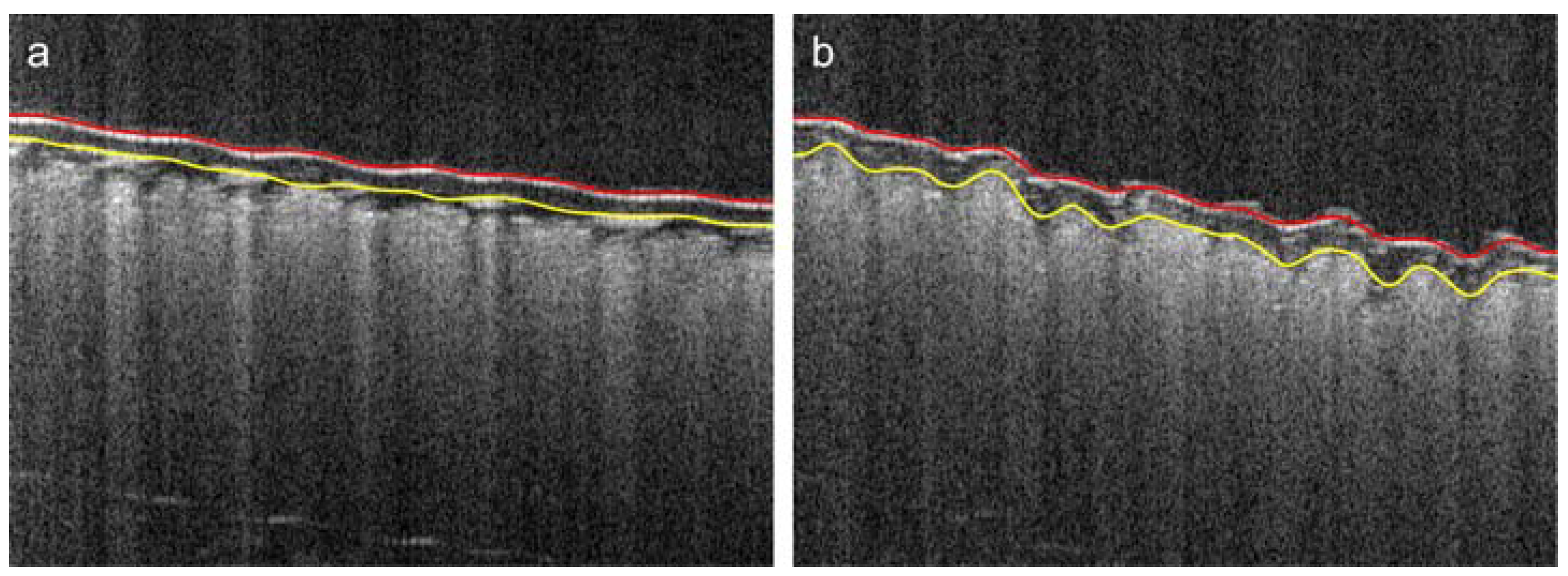
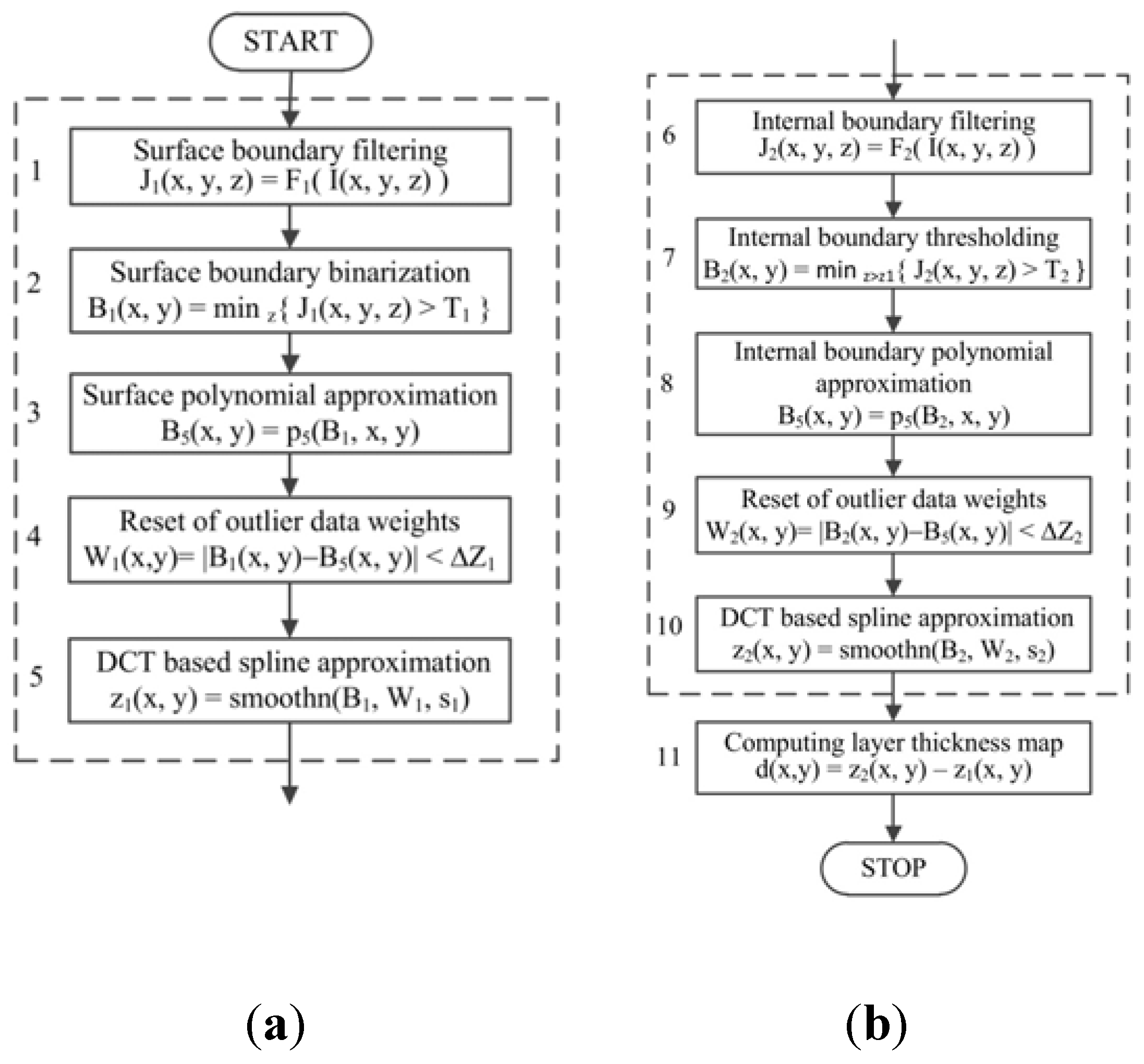
- Detection and approximation of the composite surface boundary in the XY plane of the imaging region (Figure 9a).
- Detection and approximation of the internal boundary of the composite cover layer in the XY plane of the imaging region (Figure 9b).
- Evaluation of the thickness maps of the cover layer by subtraction of the approximated boundaries (Figure 9b).
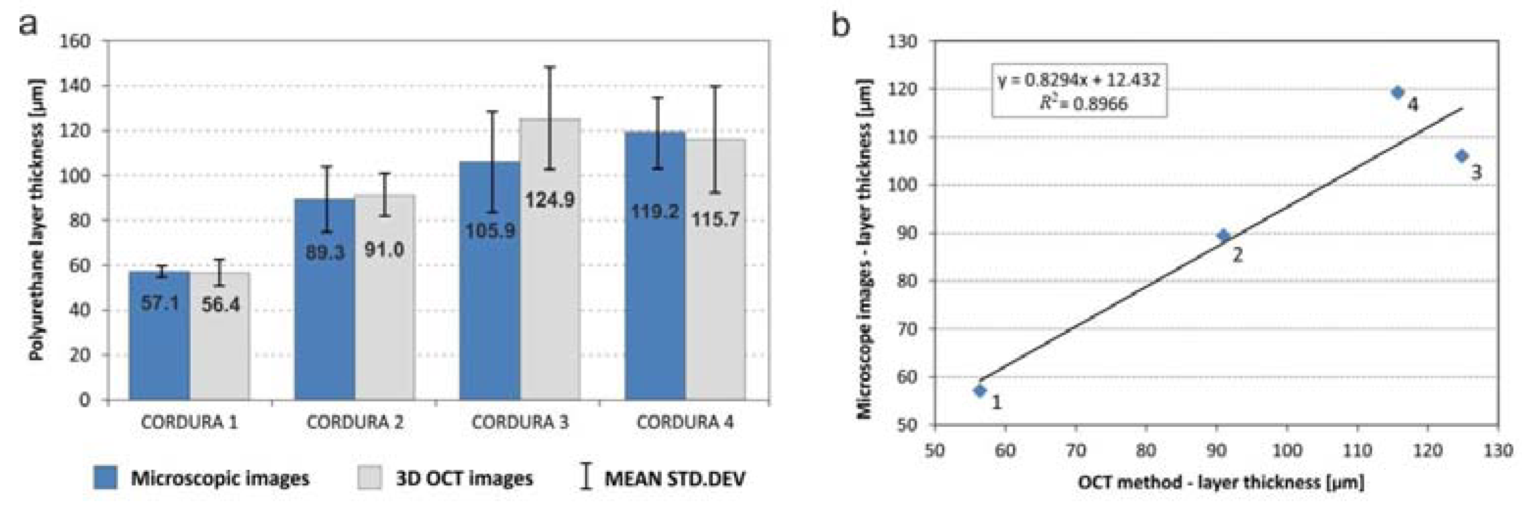
4. Results and Discussion
- = or voxels—MF filter dimensions in Equation (1) respectively for or boundary filtering,
- = or voxels—LoG filter dimensions in Equation (3) respectively for or boundary filtering,
- = voxel—standard deviations of Gaussian smoothing in LoG filter used in Equation (4),
- , —thresholds for the normalized boundary image in Equations (5) and (6), respectively,
- voxels, voxels—initial z-limit for searching the surface and internal boundaries,
- voxels—distance from the approximated surface at which to start searching for the internal boundary,
- , —the smoothing factors in Equations (12) and (14), respectively,
- equal to the doubled standard deviation of in Equation (8),
- voxels—the limit for corrected searching for the internal layer boundary.
5. Conclusions
Author Contributions
Acknowledgments
Conflicts of Interest
References
- Singha, K. A Review on Coating and Lamination in Textiles: Processes and Applications. Am. J. Polym. Sci. 2012, 2, 39–49. [Google Scholar] [CrossRef]
- Kovacevic, S.; Ujevic, D.; Brnada, S. Coated Textile Materials. In Woven Fabric Engineering; Dubrovski, P.D., Ed.; Sciyo: Rijeka, Croatia, 2010; pp. 241–254. [Google Scholar]
- Dembicky, J. Simulation of the coating process. Fibres Text. East. Eur. 2010, 18, 79–83. [Google Scholar]
- Sen, A.K. Coated Textiles: Principles and Applications; CRC Press: Florida, FL, USA, 2001. [Google Scholar]
- Potocic-Matkovic, V.M.; Skenderi, Z. Mechanical properties of polyurethane coated knitted fabrics. Fibres Text. East. Eur. 2013, 21, 86–91. [Google Scholar]
- Kos, I.; Schwarz, I.G.; Suton, K. Influence of warp density on physical-mechanical properties of coated fabric. Procedia Eng. 2014, 69, 881–889. [Google Scholar] [CrossRef]
- Huang, J.; Zhang, J.; Hao, X.; Guo, Y. Study of a new novel process for preparing and co-stretching PTFE membrane and its properties. Eur. Polym. J. 2004, 40, 667–671. [Google Scholar] [CrossRef]
- Visan, A.L.; Alexandrescu, N.; Belforte, G.; Eula, G.; Ivanov, A. Experimental researches on textile laminate materials. Ind. Text. 2012, 63, 315–321. [Google Scholar]
- Masteikaite, V.; Saceviciene, V. Study on tensile properties of coated fabrics and laminates. India J. Fibre Text. Res. 2005, 30, 267–272. [Google Scholar]
- Akovali, G. Advances in Polymer Coated Textiles; Smithers Rapra: Shawbury, UK, 2014. [Google Scholar]
- Cho, J.W.; Jung, J.C.; Chun, B.C.; Chung, Y.C. Water vapor permeability and mechanical properties of fabrics coated with shape-memory polyurethane. J. Appl. Polym. Sci. 2004, 92, 2812–2816. [Google Scholar] [CrossRef]
- Jeong, J.; Lim, Y.; Parka, J. Improving thermal stability and mechanical performance of polypropylene/polyurethane blend prepared by radiation-based techniques. Eur. Polym. J. 2017, 94, 366–375. [Google Scholar] [CrossRef]
- Korzeniewska, E.; Walczak, M.; Rymaszewski, J. Elements of elastic electronics created on textile substrate. In Proceedings of the 24th International Conference on Mixed Design of Integrated Circuits and Systems, Bydgoszcz, Poland, 22–24 June 2017; pp. 447–450. [Google Scholar]
- Goddard, J.M.; Hotchkiss, J.H. Polymer surface modification for the attachment of bioactive compounds. Prog. Polym. Sci. 2007, 32, 698–725. [Google Scholar] [CrossRef]
- Hao, X.; Zhang, J.; Guo, Y. Study of new protective clothing against sars using semi-permeable PTFE/PU membrane. Eur. Polym. J. 2004, 40, 673–678. [Google Scholar] [CrossRef]
- Lam, S.J.; Wong, E.H.; Boyer, C.; Qiao, G.G. Antimicrobial polymeric nanoparticles. Prog. Polym. Sci. 2018, 76, 40–64. [Google Scholar] [CrossRef]
- Munoz-Bonilla, A.; Fernández-García, M. Polymeric materials with antimicrobial activity. Prog. Polym. Sci. 2012, 37, 281–339. [Google Scholar] [CrossRef]
- Pawlak, R.; Korzeniewska, E.; Koneczny, C.; Hałgas, B. Properties of thin metal layers deposited on textile composites by using the pvd method for textronic applications. Autex Res. J. 2017, 17, 229–237. [Google Scholar] [CrossRef]
- Pawlak, R.; Lebioda, M.; Tomczyk, M.; Rymaszewski, J.; Korzeniewska, R.; Walczak, M. Surface heat sources on textile composites—Modeling and implementation. In Proceedings of the 18th International Symposium on Electromagnetic Fields in Mechatronics, Electrical and Electronic Engineering (ISEF), Lodz, Poland, 14–16 September 2017; pp. 1–2. [Google Scholar]
- Korzeniewska, E.; Duraj, A.; Koneczny, C.; Krawczyk, A. Thin film electrodes as elements of telemedicine systems. Prz. Elektrotech. 2015, 91, 162–165. [Google Scholar] [CrossRef]
- Frydrysiak, M.; Korzeniewska, E.; Tesiorowski, Ł. The textile resistive humidity sensor manufacturing via (PVD) sputtering method. Sens. Lett. 2015, 13, 998–1001. [Google Scholar] [CrossRef]
- Stempien, Z.; Kozicki, M.; Pawlak, R.; Korzeniewska, E.; Owczarek, G.; Poscik, A.; Sajna, D. Ammonia gas sensors ink-jet printed on textile substrates. Sensors 2017. [Google Scholar] [CrossRef]
- Bistricic, L.; Baranovic, G.; Leskovac, M.; Bajsic, E.G. Hydrogen bonding and mechanical properties of thin films of polyether-based polyurethane-silica nanocomposites. Eur. Polym. J. 2010, 46, 1975–1987. [Google Scholar] [CrossRef]
- Demirel, E.; Durmaz, H.; Hizal, G.; Tunca, U. A Route toward Multifunctional Polyurethanes Using Triple Click Reactions. J. Polym. Sci. A 2016, 54, 480–486. [Google Scholar] [CrossRef]
- Reddy, K.R.; Raghu, A.V.; Jeong, H.M. Synthesis and characterization of novel polyurethanes based on 4,4′-{1,4-phenylenebis [methylylidenenitrilo]} diphenol. Polym. Bull. 2008, 60, 609–616. [Google Scholar] [CrossRef]
- Reddy, K.R.; Raghu, A.V.; Jeong, H.M. Synthesis and characterization of pyridine-based polyurethanes. Des. Monomers Polym. 2009, 12, 109–118. [Google Scholar] [CrossRef]
- Choi, S.H.; Kim, D.H.; Raghu, A.V.; Reddy, K.R.; Lee, H.I.; Yoon, K.S.; Jeong, H.M.; Kim, B.K. Properties of Graphene/Waterborne Polyurethane Nanocomposites Cast from Colloidal Dispersion Mixtures. J. Macromol. Sci. 2012, 51, 197–207. [Google Scholar] [CrossRef]
- Chen, H.; Yuan, L.; Song, W.; Wu, Z.; Li, D. Biocompatible polymer materials: Role of protein-surface interactions. Prog. Polym. Sci. 2008, 33, 1059–1087. [Google Scholar] [CrossRef]
- Son, D.R.; Raghu, A.V.; Reddy, K.R.; Jeong, H.M. Compatibility of Thermally Reduced Graphene with Polyesters. J. Macromol. Sci. 2016, 55, 1099–1110. [Google Scholar] [CrossRef]
- Han, S.J.; Lee, H.; Jeong, H.M.; Kim, B.K.; Raghu, A.V.; Reddy, K.R. Graphene Modified Lipophilically by Stearic Acid and its Composite with Low Density Polyethylene. J. Macromol. Sci. 2014, 53, 1193–1204. [Google Scholar] [CrossRef]
- Dunkers, J.P.; Parnas, R.S.; Zimba, C.G.; Peterson, R.C.; Flynn, K.M.; Fujimoto, J.G.; Bouma, B.E. Optical coherence tomography of glass reinforced polymer composites. Compos. A 1999, 30, 139–145. [Google Scholar] [CrossRef]
- Dunkers, J.P.; Phela, F.; Sanders, D.P.; Everett, M.J.; Green, W.H.; Hunston, D.L.; Parnas, R.S. The application of optical coherence tomography to problems in polymer matrix composites. Opt. Lasers Eng. 2001, 35, 135–147. [Google Scholar] [CrossRef]
- Gliscinska, E.; Sankowski, D.; Krucinska, I.; Gocławski, J.; Michalak, M.; Rowinska, Z.; Sekulska-Nalewajko, J. Optical coherence tomography image analysis of polymer surface layers in sound-absorbing fibrous composite materials. Polym. Test. 2017, 63, 194–203. [Google Scholar] [CrossRef]
- WP OCT 1300-nm: Ultra Deep Imaging. 2017. Available online: http://wasatchphotonics.com/product-category/optical-coherence-tomography/wp-oct-1300/ (accessed on 12 April 2018).
- Sanders, J.; Kandrot, E. CUDA by Example: An Introduction to General-Purpose GPU Programming, 1st ed.; Addison-Wesley: Boston, MA, USA, 2011. [Google Scholar]
- Image Processing Toolbox. 2016. Available online: http://www.mathworks.com/help/images/ (accessed on 12 April 2018).
- CUDA Toolkit Documentation v9.1.85. 2017. Available online: http://docs.nvidia.com/cuda (accessed on 12 April 2018).
- Schmitt, J.; Xiang, S.; Yung, K. Speckle in optical coherence tomography. J. Biomed. Opt. 1999, 4, 95–105. [Google Scholar] [CrossRef] [PubMed]
- Zgou, Z.; Guo, Z.; Dong, G.; Sun, J.; Zhang, D.; Wu, B. A doubly degenerate diffusion model based on the gray level indicator for multiplicative noise removal. IEEE Trans. Image Process. 2015, 24, 249–258. [Google Scholar]
- Gocławski, J.; Sekulska-Nalewajko, J. A new idea of fast three-dimensional median filtering for despeclinkg of optical coherence tomography images. Image Process. Commun. 2015, 20, 25–34. [Google Scholar] [CrossRef]
- Rogers, S. 2D Weighted Polynomial Fitting and Evaluation. 2017. Available online: https://www.mathworks.com/matlabcentral/fileexchange/13719-2d-weighted-polynomial-fitting-and-evaluation (accessed on 12 April 2018).
- Garcia, D. Robust smoothing of gridded data in one and higher dimensions with missing values. Comput. Stat. Data Anal. 2010, 54, 1167–1178. [Google Scholar] [CrossRef] [PubMed]


| Cordura No. | Trade Name | Manufacturer | Surface Weight [g/m2] |
|---|---|---|---|
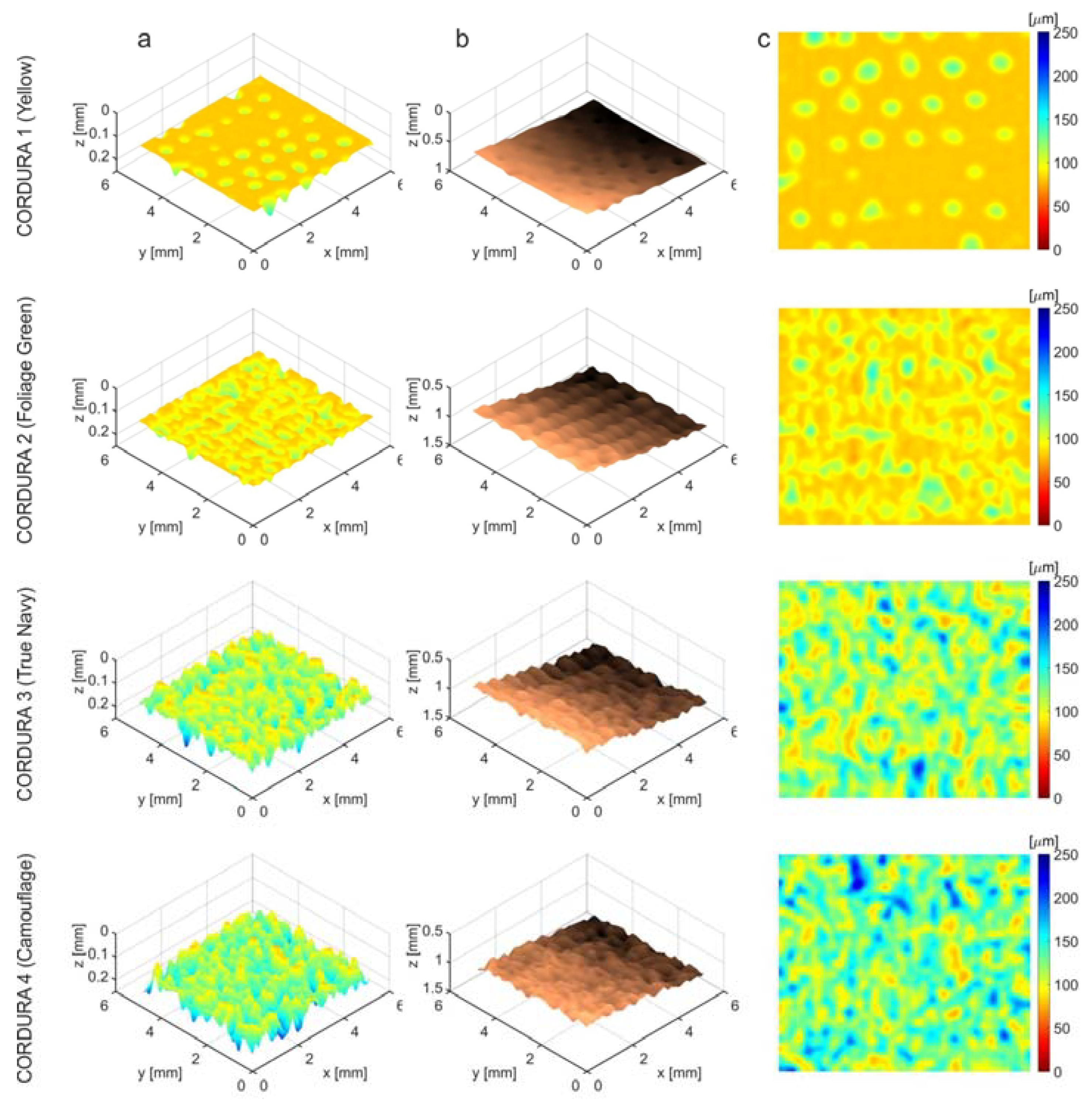
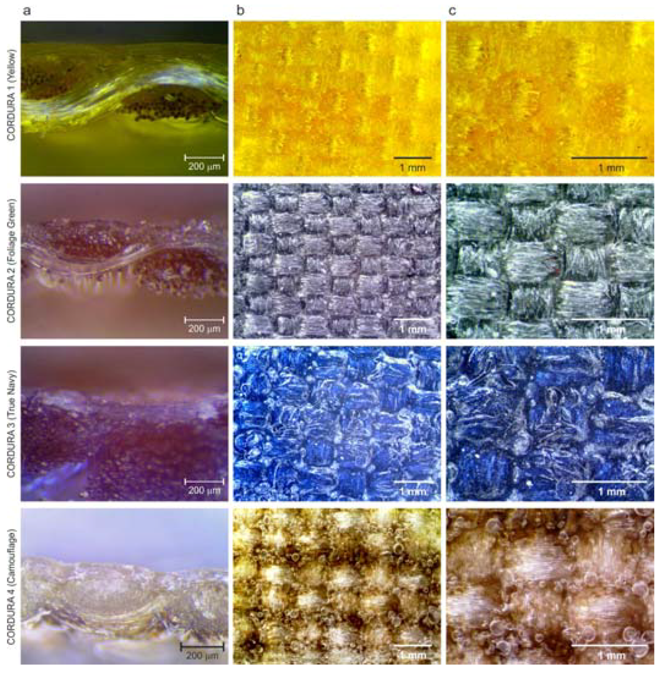
| Cordura 1 | Yellow (unknown serial number) | Miranda Ltd. Turek, Poland | 195 |
| Cordura 2 | CTD1000MS—Foliage Green | Rockwoods Ltd. Loveland, CO, USA | 380 |
| Cordura 3 | CTD1000—True Navy | Rockwoods Ltd. Loveland, CO, USA | 365 |
| Cordura 4 | Camouflage (unknown serial number) | Miranda Ltd. Turek, Poland | 460 |
| Cordura Type | [s] | [s] | [s] | [s] | [s] |
|---|---|---|---|---|---|
| 1 | 22.36 | 1.14 | 7.14 | 15.86 | 46.50 |
| 2 | 22.40 | 1.65 | 6.72 | 46.66 | 77.41 |
| 3 | 22.37 | 1.53 | 6.73 | 35.26 | 65.88 |
| 4 | 21.67 | 1.20 | 7.01 | 23.71 | 53.89 |
© 2018 by the authors. Licensee MDPI, Basel, Switzerland. This article is an open access article distributed under the terms and conditions of the Creative Commons Attribution (CC BY) license (http://creativecommons.org/licenses/by/4.0/).
Share and Cite
Gocławski, J.; Korzeniewska, E.; Sekulska-Nalewajko, J.; Sankowski, D.; Pawlak, R. Extraction of the Polyurethane Layer in Textile Composites for Textronics Applications Using Optical Coherence Tomography. Polymers 2018, 10, 469. https://doi.org/10.3390/polym10050469
Gocławski J, Korzeniewska E, Sekulska-Nalewajko J, Sankowski D, Pawlak R. Extraction of the Polyurethane Layer in Textile Composites for Textronics Applications Using Optical Coherence Tomography. Polymers. 2018; 10(5):469. https://doi.org/10.3390/polym10050469
Chicago/Turabian StyleGocławski, Jarosław, Ewa Korzeniewska, Joanna Sekulska-Nalewajko, Dominik Sankowski, and Ryszard Pawlak. 2018. "Extraction of the Polyurethane Layer in Textile Composites for Textronics Applications Using Optical Coherence Tomography" Polymers 10, no. 5: 469. https://doi.org/10.3390/polym10050469