A Revisit to the Notation of Martensitic Crystallography

Department of Materials Science and Engineering, The Ohio State University, Columbus, OH 43210, USA
Crystals 2018, 8(9), 349; https://doi.org/10.3390/cryst8090349
Submission received: 21 July 2018
/
Revised: 23 August 2018
/
Accepted: 29 August 2018
/
Published: 30 August 2018
(This article belongs to the Special Issue Microstructures and Properties of Martensitic Materials)
Abstract
:As one of the most successful crystallographic theories for phase transformations, martensitic crystallography has been widely applied in understanding and predicting the microstructural features associated with structural phase transformations. In a narrow sense, it was initially developed based on the concepts of lattice correspondence and invariant plane strain condition, which is formulated in a continuum form through linear algebra. However, the scope of martensitic crystallography has since been extended; for example, group theory and graph theory have been introduced to capture the crystallographic phenomena originating from lattice discreteness. In order to establish a general and rigorous theoretical framework, we suggest a new notation system for martensitic crystallography. The new notation system combines the original formulation of martensitic crystallography and Dirac notation, which provides a concise and flexible way to understand the crystallographic nature of martensitic transformations with a potential extensionality. A number of key results in martensitic crystallography are reexamined and generalized through the new notation.
1. Introduction
In the literature, martensitic crystallography is one of the earliest theories of phase transformations [1,2,3,4]. The fundamental concepts and mathematical treatments in martensitic crystallography are widely adopted by other crystallographic theories, such as O-lattice theory, edge-to-edge theory, structural ledge theory, invariant line theory, topological theory, etc. [5,6,7,8,9,10,11]. The starting point of martensitic crystallography is the concept of lattice correspondence, which originated from Bain’s discovery of the transformation path between face-centered cubic (FCC) and body-centered cubic (BCC) crystals in 1924 [12]. After that, two parallel theoretical branches can be distinguished. The first branch is led by the developments of Wechsler-Lieberman-Read (WLR) theory and Bowles-Mackenzie (BM) theory [13,14,15,16], in which the so-called invariant plane strain condition is introduced as a fundamental geometric constraint. Following this line, a few classic books are finished, which not only generalize the geometric constraint to compatibility condition but also establish a mathematical framework in a continuum form [1,2,3,17]. In a narrow sense, the term of classical martensitic crystallography only refers to this branch, which is usually called phenomenological theory of martensitic crystallography. On the other hand, the focus of the second branch is the change of crystal structure and symmetry during martensitic transformations [18,19,20,21]. Originating from lattice discreteness, crystal symmetry and symmetry breaking are investigated through group theory and representation theory, which leads to pathway (or state) degeneracy during martensitic transformations [22,23,24,25,26,27,28,29]. In this branch, the symmetry break is associated with a lattice correspondence connecting the initial and final crystal structures, without decomposed mathematical steps during the transformation. Despite the importance of the two theoretical branches, the connection between them was not well recognized for a long time, since distinctively different mathematical tools are utilized. However, in 2004 the intersection of the two branches was indicated in the work of Bhattacharya et al. [30] on the investigation of the reversibility of martensitic transformations. Following this work, a graph theory approach was developed to systematically analyze the transformation pathway connectivity associated with the symmetry breaking processes, which provided a general understanding of the crystallographic coupling between structural phase transformations and transformation-induced defects [31,32]. However, the mathematical connection between the two branches is still not clearly identified, partially due to the lack of a systematic notation in common. From a historical point of view, it is clear that the scope of martensitic crystallography is greatly broadened during these years, and the study of martensitic crystallography should require a combination of different mathematical tools, including linear algebra, group theory, representation theory, invariant theory, graph theory, etc. Unfortunately, the “languages” used in those mathematical tools are usually different and even inconsistent. The aim of this paper is to suggest a rigorous and consistent notation system (a common language) which can be conveniently utilized in both the above branches of martensitic crystallography theory.
As mentioned by Dirac, “a good notation can be of great value in helping the development of a theory” [33]. As a well-known example, Dirac introduced the bra-ket notation (also called Dirac notation, using symbols of “< > |”) to describe the theoretical construct of quantum mechanics in 1939, with its mathematical precursors in Grassman’s work nearly 100 years before [34]. As a convenient formulation to denote abstract vectors and linear functional in mathematics, Dirac notation plays a significant role on the development and popularization of quantum mechanics, which is broadly adopted in many textbooks. Note that Dirac notation is a mathematical notation for linear algebra, which is not necessarily associated with quantum mechanics. Theoretically, the bra-ket notation is designed for the formulation of a second-rank tensor (matrix), which describes a binary linear relation between two vectors. The advantages of bra-ket notation include: (1) abstract forms of vectors and tensor operators without specifying any basis; (2) an explicit symbol for a basis; (3) the mathematical equivalence between basis vectors and state vectors; (4) the distinction between left and right multiplications of a tensor operator; and (5) the distinction between inner and outer products. As a consequence, the formulations with bra-ket notation have a considerable flexibility in symbolic computation, which directly suggests the basis-independent nature of abstract relations. Dirac notation also has a potential extensionality to describe high-order tensors, in which more types of vectors, additional to bra and ket, could be defined in a similar way.
In the literature, the notation issue of martensitic crystallography has not been well recognized. Since most of the existing works consider the symmetry breaking to be associated with point symmetry only (within one Ericksen-Pitteri neighborhood [20,24,30]), a fixed choice of basis and reference is acceptable. In other words, all of the operators can be represented as conventional matrices in a fixed basis and a fixed reference. However, with several Ericksen-Pitteri neighborhoods taken into account, we have to involve the change among multiple bases originating from the translational symmetry of crystals, which requires a self-explanatory notation system. In the history of martensitic crystallography, there is an enlightening notation system initiated by Bowles and Mackenzie (refer as BM notation thereafter) [15], and further developed by Christian [35]. Using symbols of “( ) [ ];”, BM notation is fundamentally similar to Dirac notation, and it also provides an explicit symbol for a basis. However, brackets in BM notation always appear in pairs [15,35], while bra or ket in Dirac notation can be used individually. In other words, a basis has to be specified in BM notation, which is unnecessary in Dirac notation. In fact, the comparison between BM notation and Dirac notation does imply an antitype of notation in martensitic crystallography. Because of the lack of flexibility, BM notation has not been adopted in group theory and representation theory, which are used for the second theoretical branch.
In this paper, we suggest a new notation system to describe martensitic crystallography. A martensitic transformation between two crystal structures are considered as a binary relation between two structural states, which can also be interpreted as a second-rank tensor operator linking two sets of vectors (in which a state corresponds to a set of vectors). We reexamine the fundamental equations in martensitic crystallography and provide a number of reformulations independent of the choice of basis and reference. A concise and rigorous notation system could be of great value in helping the further development and popularization of martensitic crystallography theory.
2. Mathematical Methods and the New Notation System
For convenience, we use different types of symbols for different types of mathematical objects throughout this paper, as listed in Table 1.
In an n-dimensional vector space, we consider a crystal lattice, which can be fully described by a set of linear-independent lattice vectors:
Let us introduce the double square bracket, , to denote a structural state, with its lattice vector set indicated by A. Such a notation is a direct generalization of Dirac notation [36]. A ket describes a state vector in Dirac notation, while it describes a state vector set (a set of vectors representing a state) in our new notation. For convenience, can be defined as a combination of n column vectors, which leads to an n × n square matrix:
Parallel to the definition of bra-ket notation, can be defined as a combination of n row vectors, which also leads to an n × n square matrix:
can be considered as the transpose of . Up to now, we do not specify the basis in which (or ) is represented. In other words, the structural state of can be represented in any basis we choose, and the matrix representation of (or ) would depend on the choice of basis.
Meanwhile, the set of A itself can be regarded as a basis in the vector space. If is represented in the basis of A, we should expect an identity matrix. To make this relation consistent with the above definition, we have:
where A* is the reciprocal basis of A:
In general, a structural state represented in basis B is described by .
According to the above definitions, the following fundamental relations can be easily proved:
- (i)
- ;
- (ii)
- ;
- (iii)
- ;
- (iv)
- In particular, if A is an orthonormal basis, , so that .
The above definitions and relations are directly generalized from the inner product properties in bra-ket notation. Theoretically, when a structural state is represented in a specific basis, the associated matrix calculations are equivalent to that used in the classical theory of martensitic crystallography. However, the advantage of bra-ket notation comes from the separation of bra and ket, which provides a mathematical flexibility without specifying any basis.
If we apply an identity operator (no deformation) on state , we have:
Parallel to the definition of the outer product, we can rearrange the above equation and obtain:
In general, if we apply a deformation operator on state and obtain state , we have:
The above abstract relation, which is independent of the choice of basis, has not been directly identified in the literature, even though its physical meaning is straightforward, i.e., the lattice described by transforms into through the deformation operator . Theoretically, is a tensor operator associated with two independent bases, e.g., , and there is no constraint on the choice of C1 and C2 bases. For convenience, both state and operator are usually represented in a Cartesian coordinate system (i.e., orthonormal basis), and we use C (with possible subscript) to describe a Cartesian coordinate system. In fact, several different specific representations (tensor or matrix form) of are defined and used in the literature. For example, when C1 = C2, is the same as the deformation gradient matrix defined in continuum mechanics [2,37,38]. When is a symmetric matrix with proper choices of C1 and C2, it is named as the transformation matrix in Bhattacharya’s book [2]. Note that the symmetry of the transformation matrix is caused by the specific choice of bases, which is not an intrinsic nature of martensitic transformations. Both of the above choices of C1 and C2 rely on specific relations between C1 and C2, which are theoretically unnecessary. In the history of martensitic crystallography, the most important representation of leads to the so-called correspondence matrix [1,15,35]. For example, when is FCC and is BCC, C1 and C2 are chosen as the principal bases of the FCC and BCC lattices, respectively.
Note that the above representation of only depends on and , without any prior assumed spatial relationship or unit length relation between C1 and C2. In other words, the correspondence matrix describes a lattice correspondence relation regardless of the lattice parameters of and orientation relationship between the two lattices.
The advantage of the new notation becomes clearer when we consider the left and right multiplications of . A tensor operator on the left describes a uniform deformation on (it could be a mirror operation in a general sense).
The choice of C1 is arbitrary here.
A matrix operation on the right describes another kind of relation between the two bases. For example:
If G is a matrix belonging to the so-called general linear group GLn(Z), it can be proved that and are equivalent crystal lattices [20].
Here we need to clarify the difference between and G. and G describe two kinds of relations between two structural states. is an abstract operator (the outer product of two states), the matrix representation of which depends on the choice of the two associated bases. In contrast, G is a matrix operation (inner product) fully determined by the two states. In fact, the difference between and G originates from the definition of through column vectors (if they are row vectors, the roles of and G will be interchanged).
3. Crystallographic Results through the New Notation
In order to show the utilization of the new notation in martensitic crystallography, we arranged Section 3 in the following way. The symmetry of an individual crystal is shown in Section 3.1, while the symmetry breaking process between two crystals is discussed in Section 3.2. In Section 3.2.1 and Section 3.2.2, the symmetry breaking and pathway connectivity of martensitic transformations are analyzed, respectively, which belong to the second theoretical branch. In Section 3.2.3, kinematic compatibility condition (or invariant plane strain condition) is revisited by using the new notation, which belongs to the first theoretical branch.
3.1. Symmetry of an Individual Crystal
A crystal lattice has both point symmetry and translational symmetry. Here we consider a matrix operation , and all equivalent lattices of can be described by , without specifying any basis.
We consider an arbitrary orthogonal operator, . The point group of can be described as:
In the literature, LA is the so-called lattice group [20,22,26]. By using the property of orthogonal operator , we can eliminate in the definition of LA.
From the above equation, it is clear that the symmetry of a crystal lattice is independent of the choice of basis. is the representation of in A* basis. More mathematical details about the lattice group can be found in the literature [20,21,22,23,24,25,26,27].
Consider a point symmetry operation of lattice , with an operator . We have:
Note that is a point symmetry operator of , while GA is a point symmetry operation matrix in the lattice group of . The above equation establishes a one-to-one correspondence between the operator and matrix GA (for a given lattice ). In other words, and GA describe the same point symmetry of (or GA is another way to describe based on representation theory). However, the representation form of depends on the choice of basis, while GA can be determined without specifying any basis. In the literature of martensitic crystallography, it has not been well recognized that a few critical results are independent of the choice of basis, partially because of the lack of a scientific notation system.
3.2. Transformation between Two Crystal Lattices
From the physical point of view, there are several crystallographic phenomena associated with a martensitic transformation. First, because of the broken symmetry in the parent phase, a few crystallographically equivalent transformation pathways are generated, which leads to equivalent structural states in the product phase. Second, the transformation pathways connect multiple structural states directly or indirectly, which could establish a complex transformation pathway network, especially during forward and backward transformation cycles. Third, the generation of multiple structural states during the phase transformation produces deformed domains in crystalline materials, and the spatial arrangement of the domains raises geometric compatibility issues at the macroscopic level.
Mathematically, a transformation between two lattices, and , can be described as a mapping relation between two structural states:
The lattice groups of and are LA and LB, respectively, as determined through Equation (15). Note that LA and LB are not independent, since and are linked through in Equation (18).
3.2.1. Transformation Pathway Degeneracy
Consider a symmetry operation matrix . is a point symmetry of inherited from if and only if . In other words, considering and , and are the corresponding point symmetry operations if and only if . Furthermore, it can be proved that:
The above relation suggests equivalence between a matrix equation and an operator equation. The operator equation has been used to determined pathway degeneracy in the literature [28,29].
Here we can determine the common symmetry operations in LA and LB, which is in fact an intersection group of LA and LB (also called the stabilizer group in the literature).
During the forward transformation from to , only the symmetry operations in S are preserved, while other symmetry operations originally in LA disappear. During the backward transformation from to , only the symmetry operations in S are preserved, while other symmetry operations originally in LB disappear. As a result, the transformation pathway degeneracy (i.e., the number of equivalent transformation pathways) for and can be determined through Lagrange’s Theorem [28,29,39], as shown in Equations (21) and (22), respectively:
where indicates the order of the group S, i.e., the number of elements in S.
One special case can be easily checked with the above equations, when is an orthogonal operator, i.e., . In this case, , so that . As a result, there is no symmetry loss during the transformation between and , so that and are in fact the same structural states. A typical example of this occurs when is a rotation operator.
3.2.2. Transformation Pathway Connectivity
In the literature, the so-called phase transition graph (PTG) is introduced to capture the pathway connectivity during martensitic transformations [31]. In a PTG, each vertex corresponds to a structural state, while each edge (connecting two vertices) corresponds to a transformation pathway (between two structural states). Combined with previous results, we know that each structural state can be described by a unique matrix (i.e., ), while each edge can be described by a transformation operator (connecting states of and ). Since the definition of the lattice group LA only depends on , different structural states have different lattice groups. Because the representation of the transformation operator depends on the choice of bases, we usually use for convenience, where CA and CB are the principal bases of and , respectively. In order to construct a PTG, we start with an arbitrary state (as the reference) and calculate . Then, we calculate its connected state through the transformation operator and obtain . It is clear that both and are independent of the choice of basis. Theoretically, we can calculate other structural states one by one in this way. In fact, the choice of reference state does not affect the construction of a PTG, since we can always make a change of reference through a right multiplication matrix, e.g., , where is the new reference state and links the two structural states with an equivalent lattice.
3.2.3. Geometric Compatibility
From a mathematical point of view, all of the previous calculations are based on matrix multiplication. However, matrix addition (and subtraction) has to be involved in this part to define a compatibility condition. Note that two states (or two operators) can be added together only if they are represented in the same basis (or bases).
Here we consider the formation of a planar boundary between two neighboring domains in and . The kinematic compatibility condition (or invariant plane strain condition) can be written as [2,30]:
where b is the shear vector and n is the boundary plane normal. can be considered as a one-dimensional basis, with one non-zero vector b and two zero vectors (similar for ).
Since is the reference state (arbitrarily chosen), the above equation can be converted to operator form (with considered):
The above equation can be solved in any basis. One convenient way is to assume that the two lattices are represented in their own bases as and . As a result, the above operator equation can be represented as a matrix equation:
The unknowns to be solved in the above equation are , , and . If CA and CB1 are two Cartesian coordinate systems with the same unit length, is a rotation matrix describing the orientation relationship between the two bases (as well as the two lattices).
For a more general case, we consider the formation of a planar boundary between two neighboring domains in and . The compatibility condition can be written as:
The operator form is:
The representation in the CA basis is:
If the above equation is left multiplied by and right multiplied by , it is reduced to the same form as Equation (25). The mathematical details to solve Equations (25) and (28) are not presented here, but can be easily found in the literature [1,2,3,13,14,15,16].
Even though Equation (27) is clearly basis-independent, we have to specify a basis to solve it (e.g., Equation (28)), because the orientation relationship between the bases is a piece of output information of the kinematic compatibility condition (or invariant plane strain condition), which has to be described in a basis (the choice is arbitrary). In contrast, the solutions of other equations (e.g., Equations (13), (15), (20), (21), and (22)) do not depend on the choices of basis, which is clearly suggested by the equations formulated in our new notation.
4. Summary
Based on the existing knowledge in martensitic crystallography, we suggest a new notation system with the following major features:
- (1)
- A deformation on a crystal lattice is regarded as a linear operation on a structural state.
- (2)
- Abstract forms of states and operators are provided, without specifying any basis.
- (3)
- An explicit symbol is given to elucidate the basis (or bases) associated with a matrix representation of a state (or an operator), which makes all mathematical equations self-explanatory.
- (4)
- A series of key results in martensitic crystallography can be easily proved to be independent of the choice of basis and reference.
The new notation is applied to reexamine the fundamental problems in martensitic crystallography, which leads to concise and abstract formulations. Taking advantage of the convenience of the new notation, we would expect to reformulate martensitic crystallography in a general and rigorous framework with a potential extensionality.
Funding
This research was funded by the U.S. Department of Energy under Grant No. DE-SC0001258.
Acknowledgments
The author thanks Yunzhi Wang and Suliman A. Dregia at The Ohio State University for many fruitful discussions.
Conflicts of Interest
The author declares no conflict of interest.
Appendix A. Case Study of the Square to Hexagonal Transformation in Two Dimensions (2D)
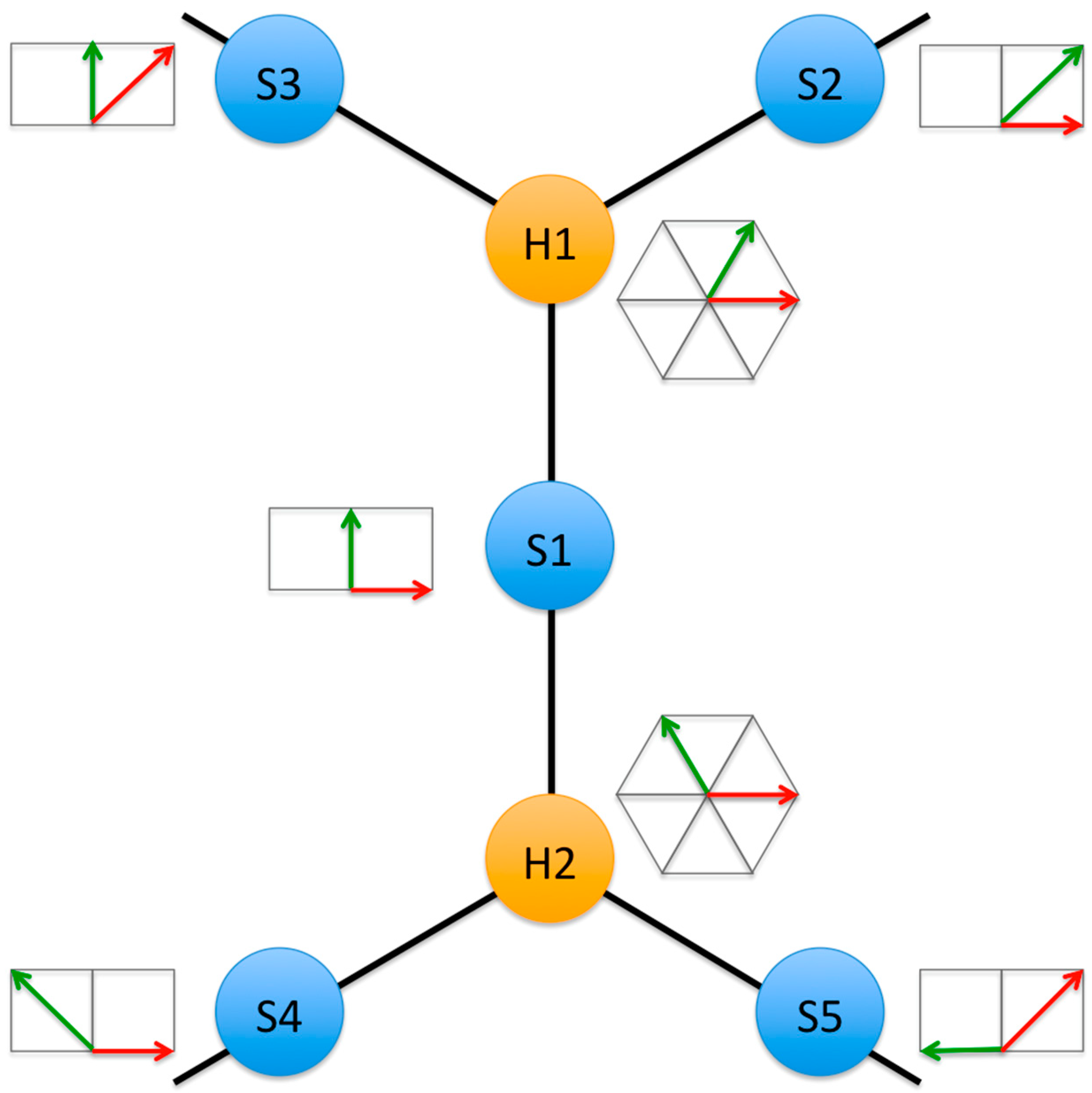
A phase transition graph for the transformation between square and hexagonal lattices is shown in Figure A1. Structural states in a square lattice (i.e., , , , and ) are represented by blue vertices, while structural states in a hexagonal lattice (i.e., and ) are represented by yellow vertices. The intrinsic link among all the states is the lattice correspondence, which is shown by corresponding vector sets. In other words, all of the vectors described by red arrows correspond to each other (similar for all the vectors described by green arrows). Starting from a square lattice, we choose two independent vectors to describe this structural state (as shown by red and green arrows near vertex S1 in Figure A1). Theoretically, the choice of the vector set defines a reference. Starting from S1, we can obtain H1 and H2 after a square to hexagonal transformation, and then S2 ~ S5 after a transformation cycle.
The crystallographic information for each structural state is listed as follows:
The point symmetry in common for and can be determined as:
Figure A1.
Phase transition graph for the square to hexagonal transformation in two dimensions (2D). The red and green arrows in each state describe two independent vectors in a 2D lattice. They also indicate the lattice correspondence among all of the structural states.
Figure A1.
Phase transition graph for the square to hexagonal transformation in two dimensions (2D). The red and green arrows in each state describe two independent vectors in a 2D lattice. They also indicate the lattice correspondence among all of the structural states.

According to Equations (21) and (22), there are two equivalent pathways for the transformation from a square to a hexagonal lattice, and three equivalent pathways from a hexagonal to a square lattice.
Note that all of the above crystallographic results are independent of the choice of basis. For example, we can calculate in S1 basis and S3 basis and compare the results.
References
- Wayman, C.M. Introduction to the Crystallography of Martensitic Transformation; Macmillan: New York, NY, USA, 1964. [Google Scholar]
- Bhattacharya, K. Microstructure of Martensite: Why It Forms and How It Gives Rise to the Shape-Memory Effect; Oxford University Press: New York, NY, USA, 2003. [Google Scholar]
- Khachaturyan, A.G. Theory of Structural Transformations in Solids; Dover Publications: New York, NY, USA, 2008. [Google Scholar]
- Otsuka, K.; Wayman, C.M. Shape Memory Materials; Camb. University Press: New York, NY, USA, 1999. [Google Scholar]
- Bollmann, W. Crystal Defects and Crystalline Interfaces; Springer: Berlin, Germany, 2012. [Google Scholar]
- Zhang, W.Z.; Weatherly, G.C. On the crystallography of precipitation. Prog. Mater. Sci. 2005, 50, 181–292. [Google Scholar] [CrossRef]
- Zhang, M.X.; Kelly, P.M. Crystallographic features of phase transformations in solids. Prog. Mater. Sci. 2009, 54, 1101–1170. [Google Scholar] [CrossRef]
- Furuhara, T.; Howe, J.M.; Aaronson, H.I. Interphase boundary structures of intragranular proeutectoid α plates in a hypoeutectoid Ti-Cr alloy. Acta Metall. Mater. 1991, 39, 2873–2886. [Google Scholar] [CrossRef]
- Dahmen, U. Orientation relationships in precipitation systems. Acta Metall. 1982, 30, 63–73. [Google Scholar] [CrossRef] [Green Version]
- Hirth, J.P.; Pond, R.C.; Hoagland, R.G.; Liu, X.Y.; Wang, J. Interface defects, reference spaces and the Frank–Bilby equation. Prog. Mater. Sci. 2013, 58, 749–823. [Google Scholar] [CrossRef]
- Howe, J.M.; Pond, R.C.; Hirth, J.P. The role of disconnections in phase transformations. Prog. Mater. Sci. 2009, 54, 792–838. [Google Scholar] [CrossRef]
- Bain, E.C. The nature of martensite. Trans. AIME 1924, 70, 25–47. [Google Scholar]
- Wechsler, M.S.; Lieberman, D.S.; Read, T. On the theory of the formation of martensite. Trans. AIME 1953, 197, 1503–1515. [Google Scholar]
- Bowles, J.S.; Mackenzie, J.K. The crystallography of martensite transformations I. Acta Metall. 1954, 2, 129–137. [Google Scholar] [CrossRef]
- Mackenzie, J.K.; Bowles, J.S. The crystallography of martensite transformations II. Acta Metall. 1954, 2, 138–147. [Google Scholar] [CrossRef]
- Bowles, J.S.; Mackenzie, J.K. The crystallography of martensite transformations III. Face-centred cubic to body-centred tetragonal transformations. Acta Metall. 1954, 2, 224–234. [Google Scholar] [CrossRef]
- Bhattacharya, K.; James, R.D. A theory of thin films of martensitic materials with applications to microactuators. J. Mech. Phys. Solids 1999, 47, 531–576. [Google Scholar] [CrossRef]
- Cahn, J.W. The symmetry of martensites. Acta Metall. 1977, 25, 721–724. [Google Scholar] [CrossRef]
- Anderson, P.W.; Blount, E.I. Symmetry considerations on martensitic transformations:” ferroelectric” metals? Phys. Rev. Lett. 1965, 14, 217. [Google Scholar] [CrossRef]
- Ericksen, J.L. Some phase transitions in crystals. Arch. Ration. Mech. Anal. 1980, 73, 99–124. [Google Scholar] [CrossRef]
- Tolédano, P.; Dmitriev, V. Reconstructive Phase Transitions: In Crystals and Quasicrystals; World Scientific Publishing Co.: Singapore, 1996. [Google Scholar]
- Fonseca, I. Variational methods for elastic crystals. Arch. Ration. Mech. Anal. 1987, 97, 189–220. [Google Scholar] [CrossRef]
- Parry, G.P. On the elasticity of monatomic crystals. Math. Proc. Camb. Philos. Soc. 1976, 80, 189–211. [Google Scholar] [CrossRef]
- Pitteri, M. Reconciliation of local and global symmetries of crystals. J. Elast. 1984, 14, 175–190. [Google Scholar] [CrossRef]
- Cayron, C. One-step model of the face-centred-cubic to body-centred-cubic martensitic transformation. Acta Cryst. A 2013, 69, 498–509. [Google Scholar] [CrossRef]
- Conti, S.; Zanzotto, G. A variational model for reconstructive phase transformations in crystals, and their relation to dislocations and plasticity. Arch. Ration. Mech. Anal. 2004, 173, 69–88. [Google Scholar] [CrossRef]
- Müller, U. Symmetry Relationships between Crystal Structures: Applications of Crystallographic Group Theory in Crystal; Oxford University Press: Oxford, UK, 2013; Volume 18. [Google Scholar]
- Cayron, C. Angular distortive matrices of phase transitions in the fcc–bcc–hcp system. Acta Mater. 2016, 111, 417–441. [Google Scholar] [CrossRef] [Green Version]
- Gao, Y.; Shi, R.; Nie, J.F.; Dregia, S.A.; Wang, Y. Group theory description of transformation pathway degeneracy in structural phase transformations. Acta Mater. 2016, 109, 353–363. [Google Scholar] [CrossRef] [Green Version]
- Bhattacharya, K.; Conti, S.; Zanzotto, G.; Zimmer, J. Crystal symmetry and the reversibility of martensitic transformations. Nature 2004, 428, 55–59. [Google Scholar] [CrossRef] [PubMed] [Green Version]
- Gao, Y.; Dregia, S.A.; Wang, Y. A universal symmetry criterion for the design of high performance ferroic materials. Acta Mater. 2017, 127, 438–449. [Google Scholar] [CrossRef]
- Gao, Y.; Casalena, L.; Bowers, M.L.; Noebe, R.D.; Mills, M.J.; Wang, Y. An origin of functional fatigue of shape memory alloys. Acta Mater. 2017, 126, 389–400. [Google Scholar] [CrossRef]
- Dirac, P.A.M. A new notation for quantum mechanics. Math. Proc. Camb. Philos. Soc. 1939, 35, 416–418. [Google Scholar] [CrossRef]
- Grassmann, H.; Kannenberg, L.C. Extension Theory; American Mathematical Society: Providence, RI, USA, 2000. [Google Scholar]
- Christian, J.W. The theory of Transformations in Metals and Alloys; ELSEVIER: Oxford, UK, 2002. [Google Scholar]
- Susskind, L.; Friedman, A. Quantum Mechanics: The Theoretical Minimum; Basic Books: New York, NY, USA, 2014. [Google Scholar]
- Ball, J.M.; James, R.D.; Smith, F.T. Proposed experimental tests of a theory of fine microstructure and the two-well problem. Philos. Trans. R. Soc. Lond. A 1992, 338, 389–450. [Google Scholar] [CrossRef]
- Ball, J.M.; James, R.D. Fine phase mixtures as minimizers of energy. Arch. Rational Mech. Anal. 1987, 100, 13–52. [Google Scholar] [CrossRef]
- Burns, G. Introduction to Group Theory with Applications: Materials Science and Technology; Academic Press: New York, NY, USA, 2014. [Google Scholar]

Table 1.
Mathematical objects and symbols.
| Objects | Symbol Description | Examples |
|---|---|---|
| Set, group | Italic upper-case letter | L |
| Matrix | Bold upper-case letter | G |
| Column vector | Bold lower-case letter | a |
| Tensor operator | Bold upper-case letter with ^ | |
| Reciprocal basis | Superscript * | A* |
| Matrix transpose | Superscript T |
© 2018 by the author. Licensee MDPI, Basel, Switzerland. This article is an open access article distributed under the terms and conditions of the Creative Commons Attribution (CC BY) license (http://creativecommons.org/licenses/by/4.0/).
Share and Cite
MDPI and ACS Style
Gao, Y. A Revisit to the Notation of Martensitic Crystallography. Crystals 2018, 8, 349. https://doi.org/10.3390/cryst8090349
AMA Style
Gao Y. A Revisit to the Notation of Martensitic Crystallography. Crystals. 2018; 8(9):349. https://doi.org/10.3390/cryst8090349
Chicago/Turabian StyleGao, Yipeng. 2018. "A Revisit to the Notation of Martensitic Crystallography" Crystals 8, no. 9: 349. https://doi.org/10.3390/cryst8090349
Note that from the first issue of 2016, this journal uses article numbers instead of page numbers. See further details here.