An Exact Method to Determine the Photonic Resonances of Quasicrystals Based on Discrete Fourier Harmonics of Higher-Dimensional Atomic Surfaces

Abstract

A rigorous method for obtaining the diffraction patterns of quasicrystals is presented. Diffraction patterns are an essential analytical tool in the study of quasicrystals, since they can be used to determine their photonic resonances. Previous methods for approximating the diffraction patterns of quasicrystals have relied on evaluating the Fourier transform of finite-sized super-lattices. Our approach, on the other hand, is exact in the sense that it is based on a technique that embeds quasicrystals into higher dimensional periodic hyper-lattices, thereby completely capturing the properties of the infinite structure. The periodicity of the unit cell in the higher dimensional space can be exploited to obtain the Fourier series expansion in closed-form of the corresponding atomic surfaces. The utility of the method is demonstrated by applying it to one-dimensional Fibonacci and two-dimensional Penrose quasicrystals. The results are verified by comparing them to those obtained by using the conventional super-lattice method. It is shown that the conventional super-cell approach can lead to inaccurate results due to the continuous nature of the Fourier transform, since quasicrystals have a discrete spectrum, whereas the approach introduced in this paper generates discrete Fourier harmonics. Furthermore, the conventional approach requires very large super-cells and high-resolution sampling of the reciprocal space in order to produce accurate results leading to a very large computational burden, whereas the proposed method generates accurate results with a relatively small number of terms. Finally, we propose how this approach can be generalized from the vertex model, which assumes identical particles at all vertices, to a more realistic case where the quasicrystal is composed of different atoms.

1. Introduction

A crystal is defined as a solid having an essentially discrete diffraction pattern [1]. In 1984, Dr. Daniel Shechtman reported that the electron diffraction pattern of a rapidly solidified alloy of aluminum (Al) and manganese (Mn) displayed a discrete spectrum and five-fold rotational symmetry [2]. The discrete diffraction peaks satisfied the definition of a crystal; however, mathematically, five-fold rotational symmetry could not be produced by a strictly periodic lattice [1]. His results were highly controversial and met with great resistance in the academic community, since it was a commonly-held belief that all crystals possessed translational symmetry. Over the next decade, several other groups reported similar observations, and this new class of crystals that lacked periodicity came to be known as quasicrystals (QCs). In recent years, there has been considerable interest in utilizing quasicrystalline morphologies in a wide range of applications, such as surface-enhanced Raman scattering (SERS) substrates [3], electronic band gap materials [4,5,6], ultra-wideband antenna arrays [7,8,9] and broadband plasmonic enhancement [10,11,12].

The diffraction patterns of QC lattices consist of discrete, Bragg-like peaks. The presence of discrete Bragg peaks suggests that, similar to periodic lattices, QCs possess photonic resonances. Additionally, due to their unique properties, QC lattices can possess multiple photonic resonances in close proximity. These properties of QC lattices make them excellent candidates for a wide variety of broadband optical applications, such as SERS substrates or broadband absorbers. Recently, plasmon-assisted coatings have been proposed to enhance the efficiency of solar cells [13]. Using QC plasmonic lattices in solar cells can enhance the absorption spectra. Moreover, due to the higher orders of symmetry, the response will be more isotropic and polarization insensitive [14].

A significant obstacle in studying QCs is the lack of analytical tools to accurately and efficiently model them. An indispensable tool for analyzing the resonant properties of QCs is their diffraction pattern. The diffraction patterns of QCs have been successfully used to predict their photonic resonances [12,15,16]. It has been shown that discrete peaks in the diffraction pattern can be associated with vectors in the reciprocal space, referred to as “reciprocal vectors” (RVs). These RVs can be directly associated with photonic resonances of QC lattices [16,17]. Thus, obtaining accurate diffraction patterns for QCs is essential, since they can be used to predict their resonances.

There is a close relationship between QCs and certain aperiodic tilings of the one-dimensional (1D) and two-dimensional (2D) plane [1]. Aperiodic tilings are generated from a set of prototiles and placing the prototiles next to each other according to a given set of matching rules. Alternatively, aperiodic tilings can be generated using a process known as Stone inflation. Stone inflation, also sometimes referred to as inflate-and-substitute, specifies how each prototile is first expanded by a given factor and then subdivided into smaller prototiles [18]. Other examples include the Danzer [1] aperiodic tiling, which possesses seven-fold rotational symmetry and the Ammann–Beenker aperiodic tiling with eight-fold rotational symmetry [18]. Converting an aperiodic tiling to a point lattice simply requires placing points at the vertices of the tiling.

The Fourier diffraction pattern of a QC is traditionally obtained by applying a Fourier transform (FT) to a finite-sized point lattice based on the QC morphology and subsequently sampling the reciprocal space to capture all of the diffraction spots. This traditional approach can often lead to inaccurate results due to the fact that the reciprocal space of QCs is densely filled [19]. To obtain an accurate diffraction pattern, two requirements must be taken into account:

(1)

The approach attempts to capture the properties of an infinite structure with a finite lattice. Thus, the truncated lattice must be large enough to display the long-range order characteristics of the QC.

(2)

The reciprocal space of QCs is densely filled [19]; thus, the sampling of the FT must be performed with a very fine resolution to capture all of the diffraction spots.

Besides the fact that this approach is often computationally expensive, it can produce inaccurate results since it attempts to capture the properties of an infinite structure by only considering a finite subset of it. Another challenge that will be examined later is that using larger and larger lattices as indicated by Requirement #1 will lead to narrower, delta-like peaks in the reciprocal space that can only be detected by increasing the sampling rate in #2, which further compounds the computational burden of this approach. We will demonstrate this problem more clearly in the next section.

In this paper, we present a novel and rigorous method to generate the diffraction patterns of QCs based on the so-called higher dimensional approach, which captures all of the properties and symmetries of the entire infinite structure by a single unit cell in higher dimensional space [20]. The QC lattices are generated by taking 1D or 2D irrational slices of higher dimensional periodic hyper-lattices. Formally, this method is referred to as the cut-and-project method [20]. The dimensionality of the hyper-lattice corresponds to the rotational symmetry of the QC. While mathematically more involved, this approach elegantly captures all of the symmetries of the QC lattice within a unit cell of the hyper-lattice [18].

Here, we present a rigorous method of obtaining the diffraction pattern of a QC based on the Fourier series (FS) expansion of the higher dimensional unit cell, which leads to discrete harmonics. Unlike the traditional methods, which apply a FT to a finite-sized supper-lattice, our method is capable of capturing the exact diffraction pattern corresponding to an infinite QC lattice. To demonstrate the validity of our approach, we present two examples. First, we consider a 1D Fibonacci QC, which can be obtained as an irrational slice of a 2D periodic lattice. Next, we consider a 2D Penrose QC, which can be obtained either as a 2D slice of a 5D hyper-cubic lattice [20] or as a 2D slice of a 4D root lattice $A_4$ [21]. Here, we employ the 4D root lattice in our derivations, since it reduces the computational burden of the problem.

2. Quasicrystals

As was noted earlier, crystals are identified by their discrete diffraction pattern. Mathematically, there is a close relationship between diffraction patterns and the FT of point lattices. The Dirac delta function introduces a convenient way to represent a set of scatterers as a summation of infinitesimal points. We start by considering $\Lambda =\left\{{\overrightarrow{x}}_1,{\overrightarrow{x}}_2,\dots \right\}$ as a discrete set of points in n-dimensional Euclidean space $E^n$ where ${\overrightarrow{x}}_k$ is an n-dimensional vector representing the location of the k-th point in Λ. The FT of this lattice denoted by $\widehat{f}\left(\overrightarrow{s}\right)$ is obtained from the following integral:

$$\widehat{f}\left(\overrightarrow{s}\right)={\int }_{R^n}f\left(\overrightarrow{x}\right)exp\left(-2\pi i\overrightarrow{x}·\overrightarrow{s}\right)\mathrm{d}\overrightarrow{x}$$

(1)

where $i=\sqrt{-1}$. It can easily be shown that for an infinite periodic lattice, the FT in Equation (1) becomes a discrete periodic impulse train or in essence, it becomes a FS. A periodic point lattice is said to possess translational symmetry, since a translation mapping by any integer summation of lattice vectors will map the lattice onto itself. Another property associated with crystals is their rotational symmetry. The rotational symmetry of a crystal is defined in terms of the rotational symmetry of its diffraction pattern. Thus, if the diffraction pattern of a point set is unchanged by a $\frac{2\pi }{n}$ rotation, the point set is said to possess n-fold rotational symmetry. According to the crystallographic restriction theorem, rotational symmetries of order five and those greater than six are impossible for diffraction patterns of periodic lattices existing in 2D and 3D space [1].

The Fibonacci QC is an example of a 1D QC. A Fibonacci sequence can be obtained iteratively from the alphabet set $\left\{A,B\right\}$, using the substitution rule: $A\to AB$, $B\to A$. Traditionally, $F_n$ denotes the Fibonacci sequence obtained after n iterative substitutions starting with $F_0=B$ [18]:

$$F_0=B,F_1=A,F_2=AB,F_3=ABA,\cdots$$

(2)

Generating a Fibonacci point lattice from a Fibonacci sequence is accomplished by assigning a thickness α, β to A and B, respectively, such that $\frac{\alpha }{\beta }=\tau$ where $\tau =\left(1+\sqrt{5}\right)/2$ is the golden ratio [1] and placing points at all junctions. Figure 1 shows the normalized diffraction pattern of a Fibonacci lattice with 4181 point scatterers, which corresponds to $F_{18}$, as defined in Equation (2). The diffraction pattern is obtained as the magnitude of the FT defined in Equation (1) where the reciprocal space region $-10\le s\le 10$ has been sampled at 100,001 equidistant points.

The Penrose QC, which is obtained from the Penrose aperiodic tiling, is an example of a 2D QC. The Penrose aperiodic tiling was discovered by Sir Roger Penrose in 1974 [22]. The Penrose lattice prototiles consist of a narrow (vertex angles $\pi /4$ and $4\pi /5$), shown in Figure 2a, and a wide (vertex angles $2\pi /5$ and $3\pi /5$) rhombi tile, shown in Figure 2b, of identical sides. The tiling, shown in Figure 2c, is obtained based on specific matching rules, which requires aligning arrows and double arrows, while pacing prototiles next to each other. As noted earlier, the tiling is converted to a point lattice simply by placing points at the vertices of the tiling. Figure 3 shows the normalized FT (magnitude) of a Penrose lattice of 711 point scatterers obtained from a Penrose tiling with tile-side of a. The diffraction pattern displayed in Figure 3 has been sampled at 501 points along $\frac{-4\pi }{a}<k_x<\frac{4\pi }{a}$ and 501 points along $\frac{-4\pi }{a}<k_y<\frac{4\pi }{a}$ for a total of ${501}^2\approx 251\times {10}^3$ points. As can be seen from Figure 3, the diffraction pattern displays five-fold rotational symmetry, which is forbidden in periodic lattices.

3. Higher Dimensional Approach

As noted earlier, the first observation of QCs was reported in X-ray diffraction patterns of rapidly solidified Al-Mn alloys, which displayed icosahedral symmetry, that is inconsistent with translational symmetry [2]. After this discovery, extensive studies took place to clarify the underlying aperiodic structure. Eventually, the most accurate models were obtained using the higher dimensional approach to derive the structure model of these icosahedral QCs [23], which completely explained their X-ray and neutron diffraction intensity. The atomic configuration was derived from a 3D section of periodic atomic surfaces in 6D space [24]. Thus, the so-called higher dimensional approach is the most rigorous method to study QCs.

The higher dimensional approach is based on the fact that a QC lattice in n-dimensional physical space $E^n$ with k-fold rotational symmetry $(k>n)$ can be embedded in a k-dimensional hyper-lattice in $E^k$ [20]. The higher dimensional space is thus referred to as the embedding space. The cut-and-project method [20], which is based on the higher dimensional approach, thus generates a QC lattice in n-dimensional space as an irrational slice of an integer hyper-lattice in $E^k$. In the cut-and-project method, the hyper-lattice is projected onto two orthogonal subspaces of dimensions n and $k-n$. The n-dimensional space ${\mathcal{E}}^{\parallel }$ is referred to as the parallel or external subspace and corresponds to the physical space. The $(k-n)$-dimensional subspace ${\mathcal{E}}^{\perp }$ is referred to as the perpendicular or internal subspace and corresponds to the unphysical space. Here, it is important to note that for a QC with k-fold rotational symmetry, k is not always the minimum dimension for the embedding space. The minimum dimension of the embedding space for a QC with k-fold rotational symmetry is $\phi \left(k\right)$, where $\phi \left(k\right)$ is Euler’s totient function, which is the number of all positive integers less than or equal to k that are relatively prime to k [18].

The higher dimensional approach elegantly restores all hidden symmetries of QCs into the unit cell of the hyper-lattice. This approach has been used to accurately calculate the band diagram of a Fibonacci photonic QC by applying Bloch’s theorem to the higher dimensional unit cell [25]. More recently, this approach has also been used to accurately and efficiently analyze diffraction from QC gratings by applying Floquet’s theorem to a higher dimensional unit cell [26]. In both cases, the results were obtained using the previously-discussed super-cell approximation approach with its stated shortcomings.

Traditionally, the diffraction patterns of QCs are obtained by first taking the FT of finite-sized point lattices and then sampling the reciprocal space to detect the peaks. We discussed the requirements for obtaining accurate diffraction patterns in the previous section and also briefly alluded to the fact that the true increased computational burden of using a larger lattice is much greater than initially expected. This is due to the fact that by definition, a crystal has a discrete diffraction pattern. By a discrete diffraction pattern, we essentially mean that the diffraction pattern is a summation of weighted Dirac delta functions. Thus, as the number of points in a crystalline (or quasicrystalline) lattice gets larger, the diffraction peaks become narrower and sharper, at infinity becoming delta functions, which in turn require sampling the reciprocal space at a higher rate to detect them, further compounding the computational burden of the problem.

4. Diffraction Patterns Based on Fourier Series Expansion of Higher Dimensional Atomic Surfaces

In [23], it was noted that the diffraction pattern of a QC can be regarded as the projection of the Fourier spectrum of the hyper-lattice onto the physical space. Here, we exploit this idea to obtain the diffraction pattern of a QC from the FS expansion of the higher dimensional unit cell rather than the FT of a finite-sized super-cell. We demonstrate the method for a Fibonacci QC and a Penrose QC. The validity of the results is confirmed by comparing them to the FT of very large periodic super-cells.

4.1. Fibonacci QC

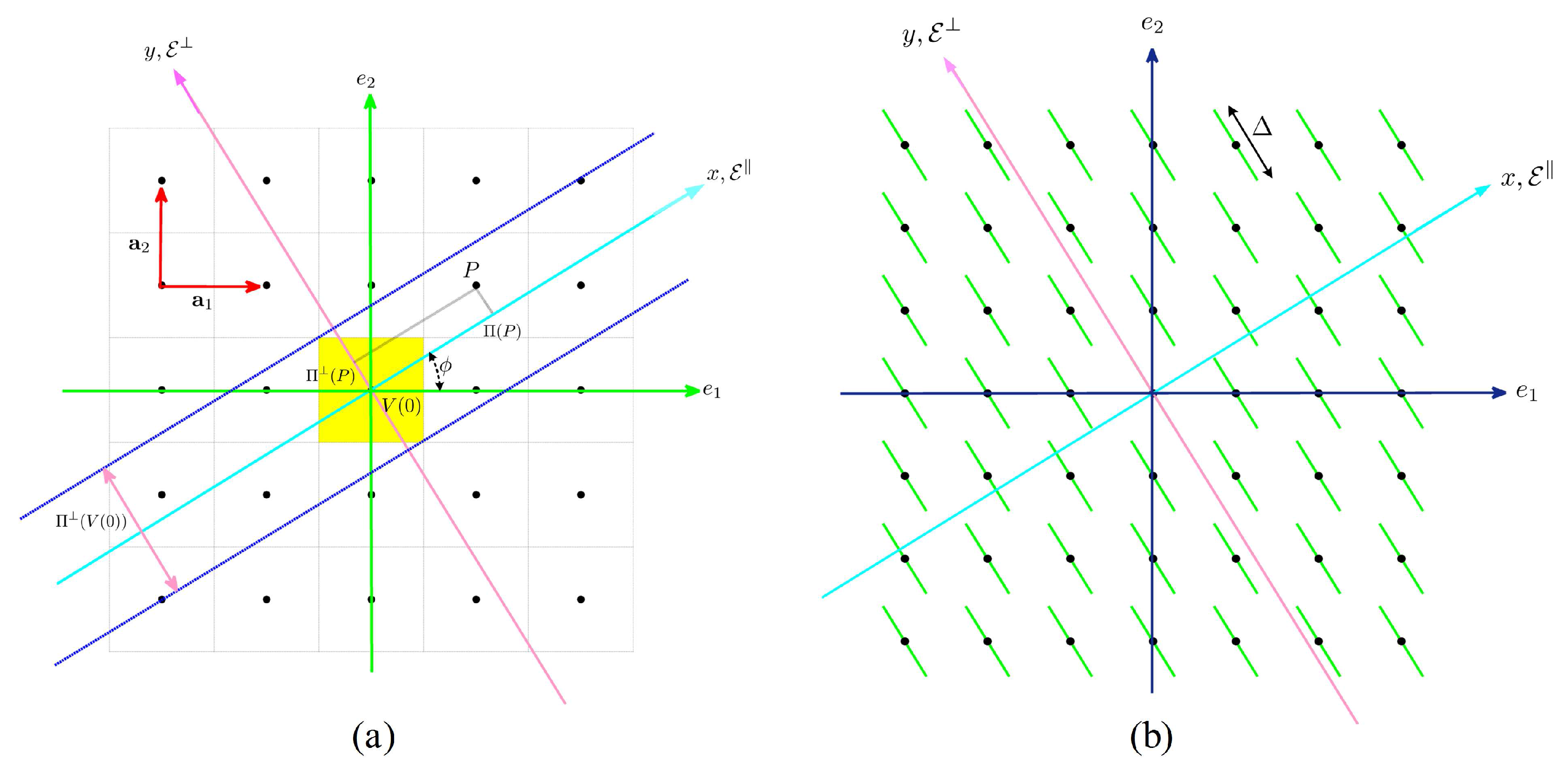
The Fibonacci QC lattice can be obtained using the cut-and-project method by taking a 1D irrational slice of a 2D periodic lattice [1], such as that shown in Figure 4a. The primitive lattice vectors are unit vectors along $e_1$ and $e_2$ denoted respectively by ${\mathbf{a}}_1$ and ${\mathbf{a}}_1$, as shown in Figure 4a, where without loss of generality, we have assumed that the lattice constant is unity. As a result, every lattice point can be represented by a set of integers. This is referred to as an integer lattice and denoted by ${\mathcal{I}}_2^p$, where the subscript 2 corresponds to the dimensionality of the lattice. The Voronoï cell at the origin is highlighted and denoted by $V\left(0\right)$.

We start by defining a new orthonormal basis with unit vectors $\widehat{\mathbf{x}}$ and $\widehat{\mathbf{y}}$ directed along x and y, as shown in Figure 4a. As can be seen, the unit vectors $\widehat{\mathbf{x}}$ and $\widehat{\mathbf{y}}$ are obtained by rotating the unit vectors ${\widehat{\mathbf{e}}}_1$ and ${\widehat{\mathbf{e}}}_2$ by an angle φ, where $tan\varphi =1/\tau$. It can easily be shown that the transformation from the ${\widehat{\mathbf{e}}}_1{\widehat{\mathbf{e}}}_2$ basis to the $\widehat{\mathbf{x}}\widehat{\mathbf{y}}$ basis can be obtained by the unitary mapping $\mathbf{M}$:

$$\mathbf{M}=\left(\begin{array}{cc}\kappa \tau & \kappa \\ \kappa & -\kappa \tau \end{array}\right)$$

(3)

where $\kappa =\frac{1}{\sqrt{1+{\tau }^2}}$. Using this mapping, the subspace x is referred to as the parallel or external subspace and is denoted by ${\mathcal{E}}^{\parallel }$. The parallel subspace corresponds to the physical space. Subspace y is referred to as the perpendicular or internal subspace and is denoted by ${\mathcal{E}}^{\perp }$. The perpendicular subspace corresponds to the unphysical space. As shown in Figure 4a, for every lattice point, P, its projection onto the parallel subspace ${\mathcal{E}}^{\parallel }$ is denoted by $\Pi \left(P\right)$, and its projection onto the perpendicular subspace ${\mathcal{E}}^{\perp }$ is denoted by ${\Pi }^{\perp }\left(P\right)$. A Fibonacci lattice can now be obtained by the projection of lattice points onto the parallel subspace ${\mathcal{E}}^{\parallel }$. However, not all lattice points are projected onto the parallel subspace, and a selection criterion is used to determine the set of lattice points that should be projected to obtain a Fibonacci QC lattice. The selection window is shown in Figure 4a as the region between two parallel lines above and below the x-axis. This region corresponds to lattice points who’s orthogonal projection onto the perpendicular subspace, denoted by ${\Pi }^{\perp }\left(P\right)$, falls inside the perpendicular projection of the Voronoï cell at the origin, which is denoted by ${\Pi }^{\perp }\left(V\left(0\right)\right)$ in Figure 4a.

An alternative way to generate QC lattices using the cut-and-project method is by decorating the lattice points with an atomic surface (AS) [18,27]. ASs are projections of the higher dimensional unit cell onto the perpendicular subspace. The points of intersection of the decorated hyper-lattice with the parallel subspace yield the QC lattice. Figure 4b shows the decorated hyper-lattice for the Fibonacci QC. The ASs are line segments of length $\Delta =sin\varphi +cos\varphi$.

Since the decorated hyper-lattice is periodic with lattice vectors ${\widehat{\mathbf{a}}}_1$ and ${\widehat{\mathbf{a}}}_2$, it can be expanded in terms of a FS:

$$\rho (e_1,e_2)=\sum _{\mathbf{G}}{c}_{\mathbf{G}}exp\left[i\mathbf{G}·\mathbf{r}\right]$$

(4)

where the sum is over all RVs $\mathbf{G}$ defined as:

$$\mathbf{G}=m_1{\mathbf{a}}_1^{*}+m_2{\mathbf{a}}_2^{*}{m}_1,m_2\in \mathbb{Z}$$

(5)

such that ${\mathbf{a}}_1^{*}$ and ${\mathbf{a}}_2^{*}$ are the primitive RVs, which are related to lattice vectors ${\widehat{\mathbf{a}}}_1$ and ${\widehat{\mathbf{a}}}_2$ by ${\mathbf{a}}_m^{*}·{\widehat{\mathbf{a}}}_k=2\pi {\delta }_{mk}$ where ${\delta }_{mk}$ is the Kronecker delta function and $\mathbf{r}=e_1{\widehat{\mathbf{a}}}_1+e_2{\widehat{\mathbf{a}}}_2$ is the position vector. It is customary to use an equal number of terms for each dimension, which we denote by N, leading to a total number of ${(2N+1)}^2$ terms in the FS. The value of the Fourier expansion coefficient $c_{\mathbf{G}}$ in Equation (4) is given by:

$$c_{\mathbf{G}}=\int {\int }_U\rho (e_1,e_2)exp\left(-i\mathbf{G}·\mathbf{r}\right)\mathrm{d}{e}_1\mathrm{d}{e}_2$$

(6)

where the integration is performed over the area of a unit cell. It is more convenient to evaluate the integral in Equation (6) in the $xy$ basis using a change of variables:

$$c_{\mathbf{G}}=\int {\int }_U\tilde{\rho }(x,y)e^{-2i\pi \kappa \left(m_1\tau x+m_{1}y+m_{2}x-m_2\tau y\right)}\mathrm{d}x\mathrm{d}y$$

(7)

where $\tilde{\rho }(x,y)$ is the AS in the $xy$ basis and can be expressed as $\tilde{\rho }(x,y)=\delta \left(x\right)\text{rect}\left(\frac{y}{\Delta }\right)$. Using this expression, we arrive at the following result for $c_{\mathbf{G}}$:

$$c_{\mathbf{G}}=\left\{\begin{array}{cc}\Delta \hfill & \text{if}\left|\mathbf{G}\right|=0\hfill \\ \frac{sin\left[\Delta \pi \kappa \left(m_1-m_2\tau \right)\right]}{\pi \kappa \left(m_1-m_2\tau \right)}\hfill & \text{if}\left|\mathbf{G}\right|\ne 0\hfill \end{array}\right.$$

(8)

Equation (8) gives the value of the Fourier harmonic $c_{\mathbf{G}}$ for the RVs $\mathbf{G}$ as defined in Equation (5). The RVs are defined with respect to the lattice vectors ${\widehat{\mathbf{a}}}_1$ and ${\widehat{\mathbf{a}}}_2$. We can also express the RVs in terms of the parallel and perpendicular subspaces as $\mathbf{G}=G_{\parallel }\widehat{\mathbf{x}}+G_{\perp }\widehat{\mathbf{y}}$ where $G_{\parallel }$ is the projection of $\mathbf{G}$ onto the parallel subspace and $G_{\perp }$ is the projection of $\mathbf{G}$ onto the perpendicular subspace. Thus, for the RVs $\mathbf{G}$ as defined in Equation (5), $G_{\parallel }$ and $G_{\perp }$ are:

$$\begin{array}{cc}\hfill G_{\parallel }& =2\pi \kappa \left(m_1\tau +m_2\right)\hfill \\ \hfill G_{\perp }& =2\pi \kappa \left(m_1-m_2\tau \right)\hfill \end{array}$$

(9)

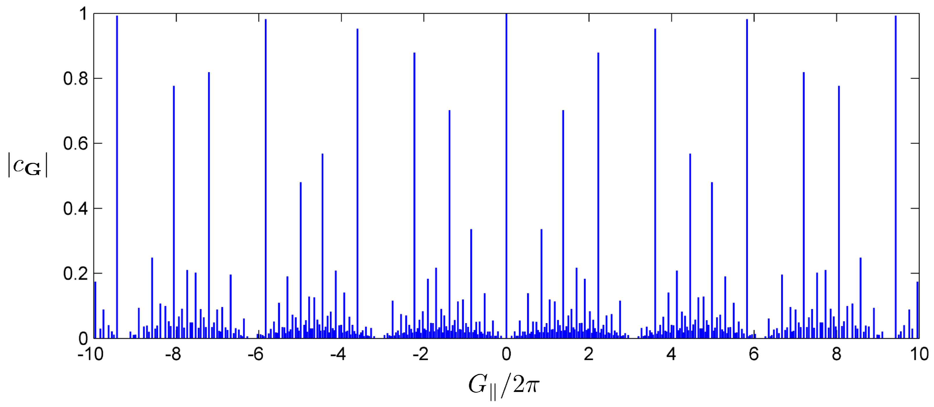
As it was noted earlier, the parallel subspace corresponds to the physical space. Hence, in the same manner that the 1D QC lattice was obtained by taking a slice of the decorated hyper-lattice along the parallel subspace, we can obtain the diffraction pattern of the QC by taking a slice of the reciprocal space of the hyper-lattice. Thus, only the parallel components of the RVs and their corresponding Fourier harmonics are considered. 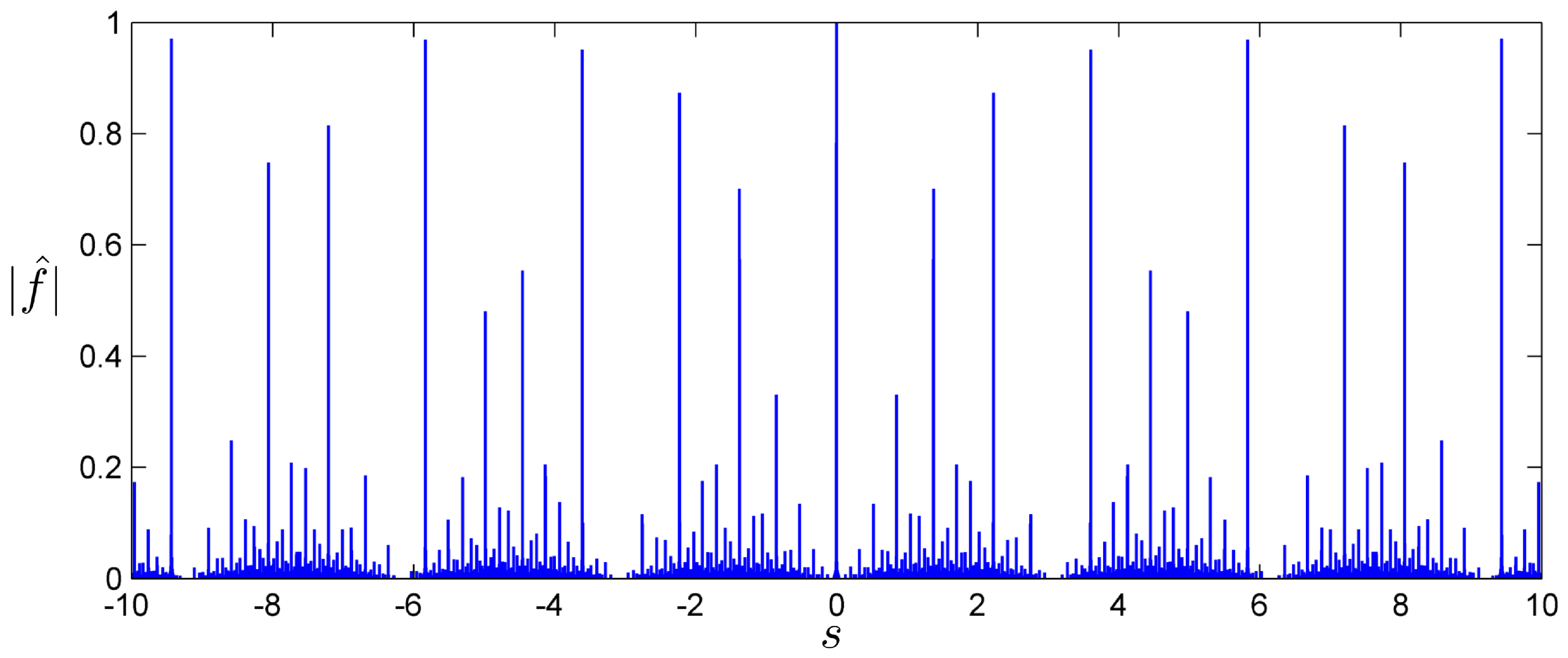Figure 5 shows the normalized diffraction pattern of the Fibonacci QC using this method. A FS expansion with 441 terms $\left(N=10\right)$ has been applied to the hyper-lattice ASs, and the resulting Fourier harmonics have been plotted versus the parallel components of the RVs. The results shown in Figure 5 can be verified by comparing them to Figure 1, which obtained the diffraction pattern by taking the FT of a very large super-cell structure.

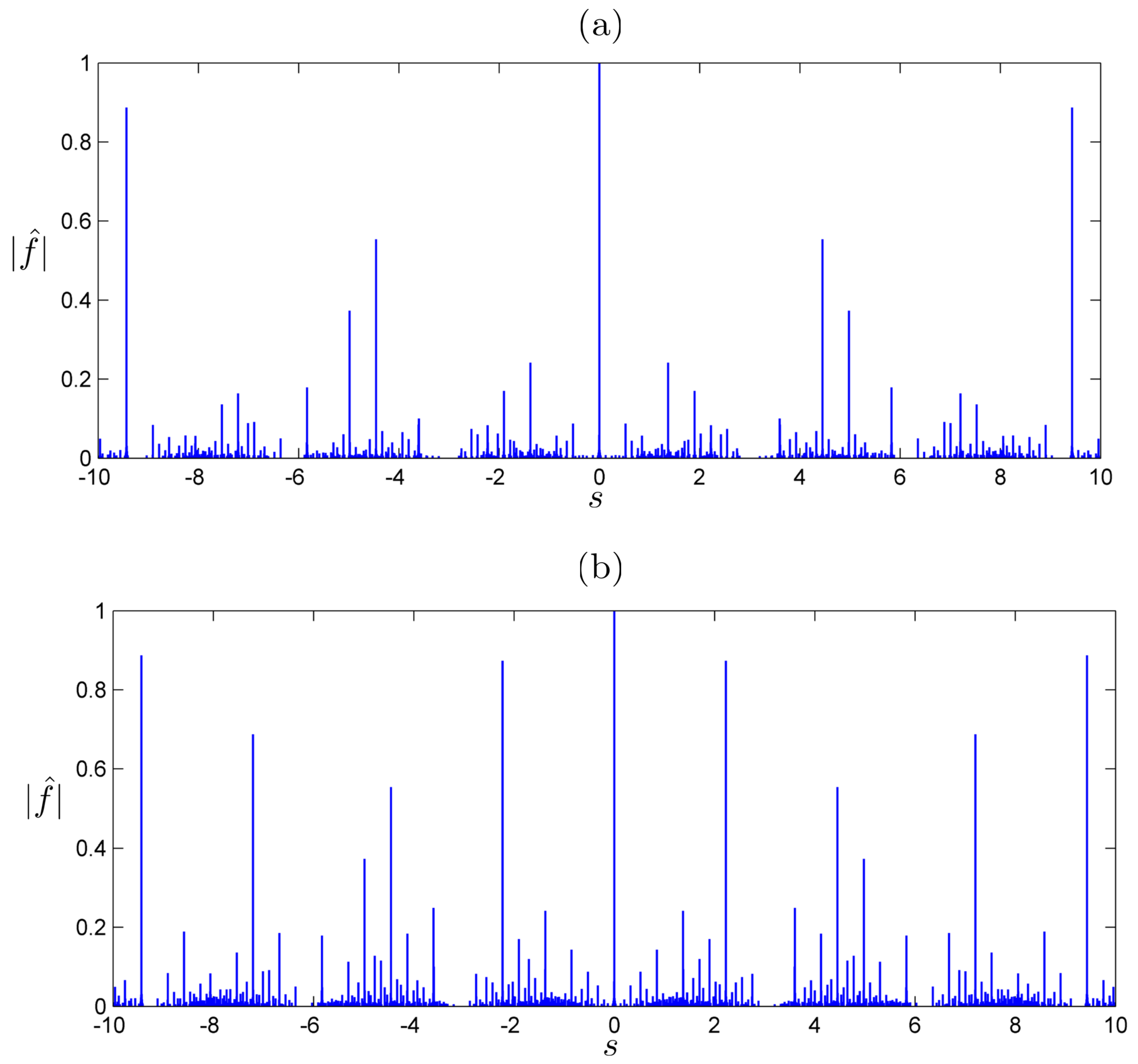
Figure 1 was obtained by evaluating the FT of a 2585 lattice at 100,001 points in the reciprocal space. As was noted, when taking the FT of a very large, but finite point lattice, it is critically important to use a very high resolution in sampling the reciprocal space, since otherwise, some strong peaks might be missed. This point is demonstrated in Figure 6. Both Figure 6a and Figure 6b correspond to the FT (magnitude) spectra of the 2585 Fibonacci lattice, which was considered previously. The only difference is that in Figure 6a, the reciprocal space has been sampled at 10,001 points, and in Figure 6b, it has been sampled at 20,001 points. As can be seen, both of these patterns lack many of the peaks shown Figure 1, which was sampled at 100,001 points.

4.2. Penrose QC

Using the cut-and-project method, the Penrose QC lattice can be obtained as a 2D slice of a 5D periodic hyper-lattice. Obtaining the Penrose QC as a 2D slice of the 5D space is known as the canonical projection, which means that the unit cell of the hyper-lattice is a 5D hyper-cube. Using this method, the hyper-cube points are mapped onto a 2D parallel space and a 3D perpendicular space. However, as was noted previously, the minimum dimension of the embedding space for a QC with k-fold rotational symmetry is $\phi \left(k\right)$, where $\phi \left(k\right)$ is Euler’s totient function and $\phi \left(5\right)=4$. Since lower dimensionality reduces the computational burden of the problem, we use the minimal space embedding to obtain our results. An important distinction between the 5D embedding and the 4D embedding is that in the case of the 4D embedding, the hyper-lattice is non-orthogonal. The 4D non-orthogonal hyper-lattice is known as the $A_4$ root lattice, and the 4D unit cell is a hyper-rhombohedral [20]. A complete discussion of the derivation of the 4D lattice is given in [18,21]. Here, we only state the results, which are important for this work. We consider the 4D Euclidean space with the standard orthonormal Euclidean basis $\left\{{\widehat{\mathbf{e}}}_1,{\widehat{\mathbf{e}}}_2,{\widehat{\mathbf{e}}}_3,{\widehat{\mathbf{e}}}_4\right\}$. The primitive lattice vectors for the $A_4$ root lattice are given by:

$$\begin{array}{cc}\hfill {\mathbf{d}}_1& =\frac{2}{\sqrt{5}}{\left[\left(c_1-1\right),s_1,\left(c_2-1\right),s_2\right]}^T\hfill \\ \hfill {\mathbf{d}}_2& =\frac{2}{\sqrt{5}}{\left[\left(c_2-1\right),s_2,\left(c_4-1\right),s_4\right]}^T\hfill \\ \hfill {\mathbf{d}}_3& =\frac{2}{\sqrt{5}}{\left[\left(c_3-1\right),s_3,\left(c_6-1\right),s_6\right]}^T\hfill \\ \hfill {\mathbf{d}}_4& =\frac{2}{\sqrt{5}}{\left[\left(c_4-1\right),s_4,\left(c_8-1\right),s_8\right]}^T\hfill \end{array}$$

(10)

where $c_j=cos\left(\frac{2j\pi }{5}\right)$ and $s_j=sin\left(\frac{2j\pi }{5}\right)$. The parallel subspace ${\mathcal{E}}^{\parallel }$ is the plane spanned by ${\widehat{\mathbf{e}}}_1{\widehat{\mathbf{e}}}_2$, and the perpendicular subspace ${\mathcal{E}}^{\perp }$ is the plane spanned by ${\widehat{\mathbf{e}}}_3{\widehat{\mathbf{e}}}_4$. The AS consists of four pentagons in the perpendicular subspace ${\mathcal{E}}^{\perp }$, which we denote by $A,B,C,$ and D. The $A,B,C,$ and D of the AS are respectively centered at points ${\mathbf{d}}_s/5,2{\mathbf{d}}_s/5,3{\mathbf{d}}_s/5,$ and $4{\mathbf{d}}_s/5$, where ${\mathbf{d}}_s={\mathbf{d}}_1+{\mathbf{d}}_2+{\mathbf{d}}_3+{\mathbf{d}}_4$ is the body diagonal of the unit cell. The mapping matrix $\mathbf{M}$ from the lattice basis to the Euclidean basis is:

$$\mathbf{M}=\frac{2}{\sqrt{5}}\left(\begin{array}{cccc}{c}_1-1& c_2-1& c_3-1& c_4-1\\ s_1& s_2& s_3& s_4\\ c_2-1& c_4-1& c_6-1& c_8-1\\ s_2& s_4& s_6& s_8\end{array}\right)$$

(11)

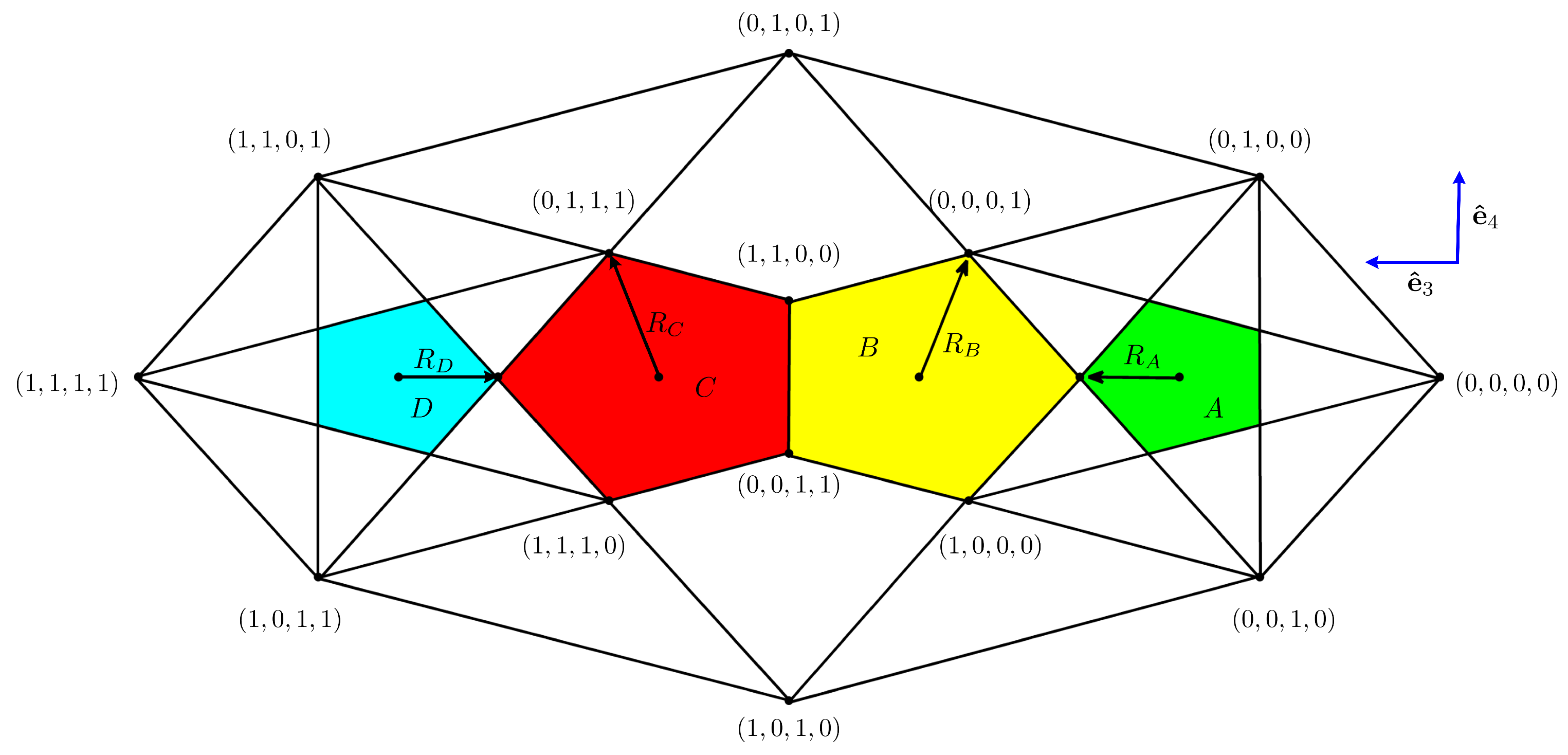
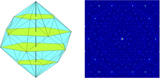
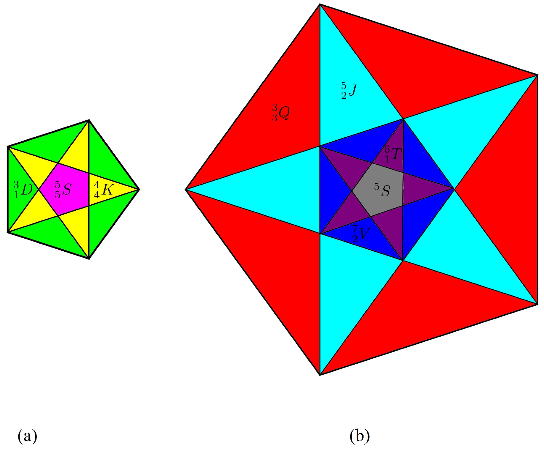
Figure 7 shows the projection of the hyper-rhombohedral unit cell onto the perpendicular space ${\mathcal{E}}^{\perp }$. Each vertex is denoted by its coordinate in the $\left\{{\mathbf{d}}_1,{\mathbf{d}}_2,{\mathbf{d}}_3,{\mathbf{d}}_4\right\}$ basis. The four ASs have been highlighted and the perpendicular space basis vectors ${\widehat{\mathbf{e}}}_3$ and ${\widehat{\mathbf{e}}}_4$ have been shown for reference. The radii of the pentagons are [18]:

$$R_A=R_D=\frac{2}{{\tau }^2\sqrt{5}},R_B=R_C=\frac{2}{\tau \sqrt{5}}$$

(12)

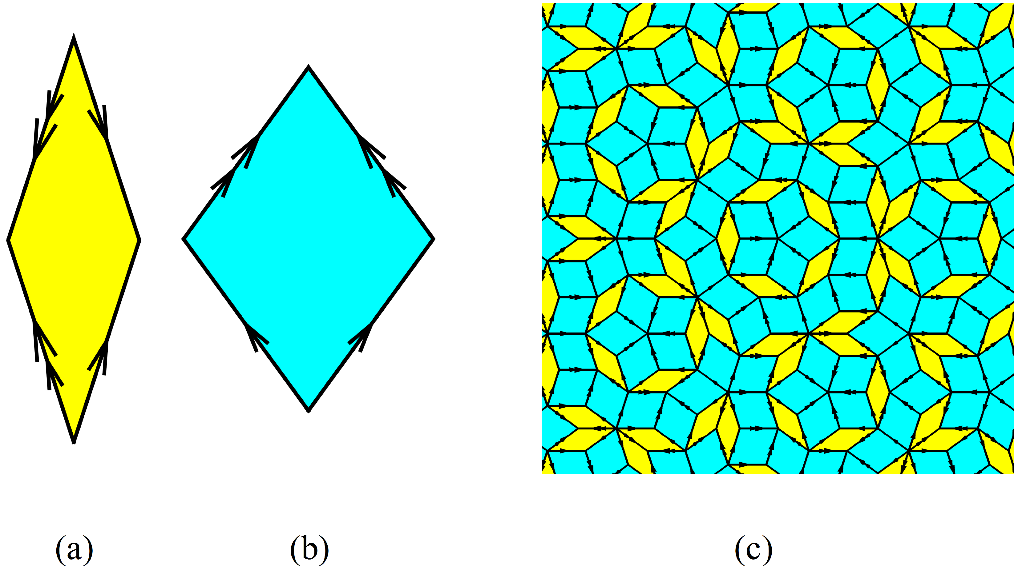
Taking a 2D slice along the parallel space of the 4D hyper-lattice will generate a Penrose QC lattice, where the tile side is $2{\tau }^2/\sqrt{5}$ [18].

At this point, it is desired to obtain the FS expansion of our higher dimensional unit cell. To accomplish this goal, the periodic AS can be expanded in terms of Fourier harmonics:

$$\rho (r_1,r_2,r_3,r_4)=\sum _{\mathbf{G}}{c}_{\mathbf{G}}exp\left[i\mathbf{G}·\mathbf{r}\right]$$

(13)

where the sum is over all RVs $\mathbf{G}$ defined as:

$$\mathbf{G}=m_1{\mathbf{d}}_1^{*}+m_2{\mathbf{d}}_2^{*}+m_3{\mathbf{d}}_3^{*}+m_4{\mathbf{d}}_4^{*}{m}_1,\dots ,m_4\in \mathbb{Z}$$

(14)

and $\mathbf{r}$ is the 4D position vector given by:

$$\mathbf{r}=r_1{\mathbf{d}}_1+r_2{\mathbf{d}}_2+r_3{\mathbf{d}}_3+r_4{\mathbf{d}}_4{d}_1,\dots ,d_4\in \mathbb{R}$$

(15)

As before, for practical reasons, the infinite expansion is truncated to the finite set of RVs defined as:

$$\mathbf{G}=\left\{m_1{\mathbf{d}}_1^{*}+m_2{\mathbf{d}}_2^{*}+m_3{\mathbf{d}}_3^{*}+m_4{\mathbf{d}}_4^{*}:\left|m_1\right|,\dots \left|m_4\right|\le N\right\}$$

(16)

which leads to a total of ${\left(2N+1\right)}^4$ terms. The value of the Fourier harmonic coefficient $c_{\mathbf{G}}$ in Equation (4) can be determined from:

$$c_{\mathbf{G}}=\frac{1}{\left|det\left(\mathbf{M}\right)\right|}\int \left\{\rho (r_1,r_2,r_3,r_4)exp\left(-i\mathbf{G}·\mathbf{r}\right)\mathrm{d}{r}_1\mathrm{d}{r}_2\mathrm{d}{r}_3\mathrm{d}{r}_4\right\}$$

(17)

where the integration is performed over the 4D $A_4$ root lattice. The term $\left|det\left(\mathbf{M}\right)\right|$ corresponds to the volume of the unit cell, which due to non-orthogonality, is not unity and must be accounted for. It is more convenient to evaluate the integral in Equation (17) in the $\left\{{\widehat{\mathbf{e}}}_1,{\widehat{\mathbf{e}}}_2,{\widehat{\mathbf{e}}}_3,{\widehat{\mathbf{e}}}_4\right\}$ basis. Applying a change of variables to Equation (17), we arrive at:

$$c_{\mathbf{G}}=\int \left\{\tilde{\rho }(e_1,e_2,e_3,e_4)e^{-2\pi i\left(m_1{d}_1+m_2{d}_2+m_3{d}_3+m_4{d}_4\right)}\mathrm{d}{e}_1\mathrm{d}{e}_2\mathrm{d}{e}_3\mathrm{d}{e}_4\right\}$$

(18)

where $\tilde{\rho }(e_1,e_2,e_3,e_4)$ is the AS in the $\left\{{\widehat{\mathbf{e}}}_1,{\widehat{\mathbf{e}}}_2,{\widehat{\mathbf{e}}}_3,{\widehat{\mathbf{e}}}_4\right\}$ basis. As shown in Figure 7, the AS surface of the 4D hyper-lattice consists of four pentagons, which lie in the perpendicular space ${\mathcal{E}}^{\perp }$. The centers for ASs $A,B,C$ and D in the $\left\{{\widehat{\mathbf{e}}}_1,{\widehat{\mathbf{e}}}_2,{\widehat{\mathbf{e}}}_3,{\widehat{\mathbf{e}}}_4\right\}$ basis, respectively, are $\left(\vartheta ,0,\vartheta ,0\right),\left(2\vartheta ,0,2\vartheta ,0\right),\left(3\vartheta ,0,3\vartheta ,0\right)$ and $\left(4\vartheta ,0,4\vartheta ,0\right)$, where $\vartheta =\frac{-2}{\sqrt{5}}$. The AS of the 4D hyper-lattice can be represented as the sum of four pentagonal ASs, as shown in Figure 7. The linearity property of the FS expansion can be exploited to evaluate the expansion for each ASs separately. Evaluating individual FS terms requires performing double integration over the area of a pentagon. While this could be performed numerically, we were able to derive analytical expressions, which improved the calculation time by almost three orders of magnitude. The derivations for the analytical results are included in the Appendix. Using these results, we can now evaluate the Fourier harmonic coefficient $c_{\mathbf{G}}$ for each RV $\mathbf{G}$ in closed-form. However, as was done in the case of the Fibonacci QC, we only need to consider the parallel component of each RV, which corresponds to the physical space. For RV $\mathbf{G}$ as defined in Equation (14), the parallel space component, denoted by ${\mathbf{G}}_{\parallel }$, is a 2D vector in the $e_1{e}_2$ plane given by:

$${\mathbf{G}}_{\parallel }=\frac{2\pi }{\sqrt{5}}\left[\begin{array}{c}{m}_1{c}_1+m_2{c}_2+m_3{c}_3+m_4{c}_4\\ m_1{s}_1+m_2{s}_2+m_3{s}_3+m_4{s}_4\end{array}\right]$$

(19)

such that the first element of the ${\mathbf{G}}_{\parallel }$ corresponds to projection along ${\widehat{\mathbf{e}}}_1$ and the second element corresponds to projection along ${\widehat{\mathbf{e}}}_2$, where at this point, we can associate ${\widehat{\mathbf{e}}}_1$ and ${\widehat{\mathbf{e}}}_2$ with the Cartesian dimensions of the physical space.

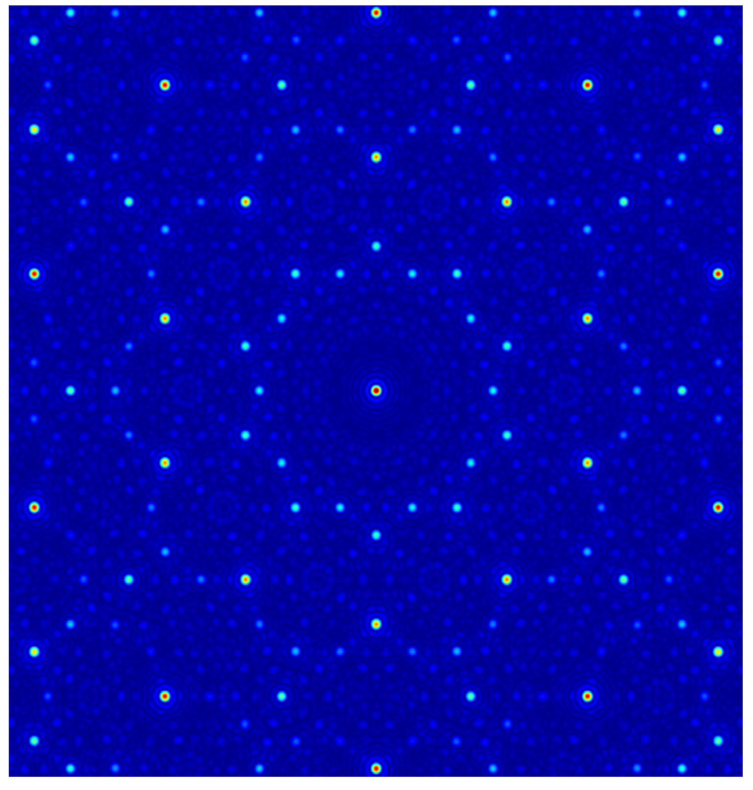
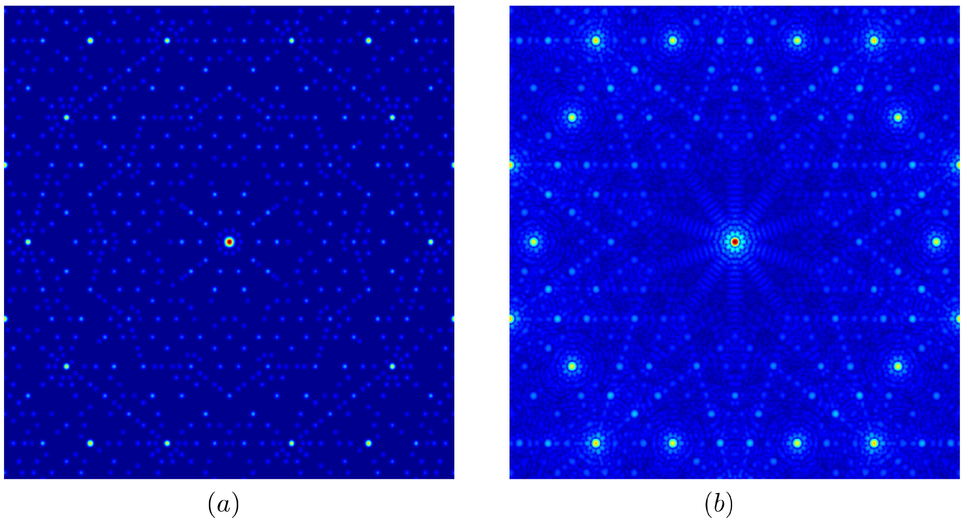
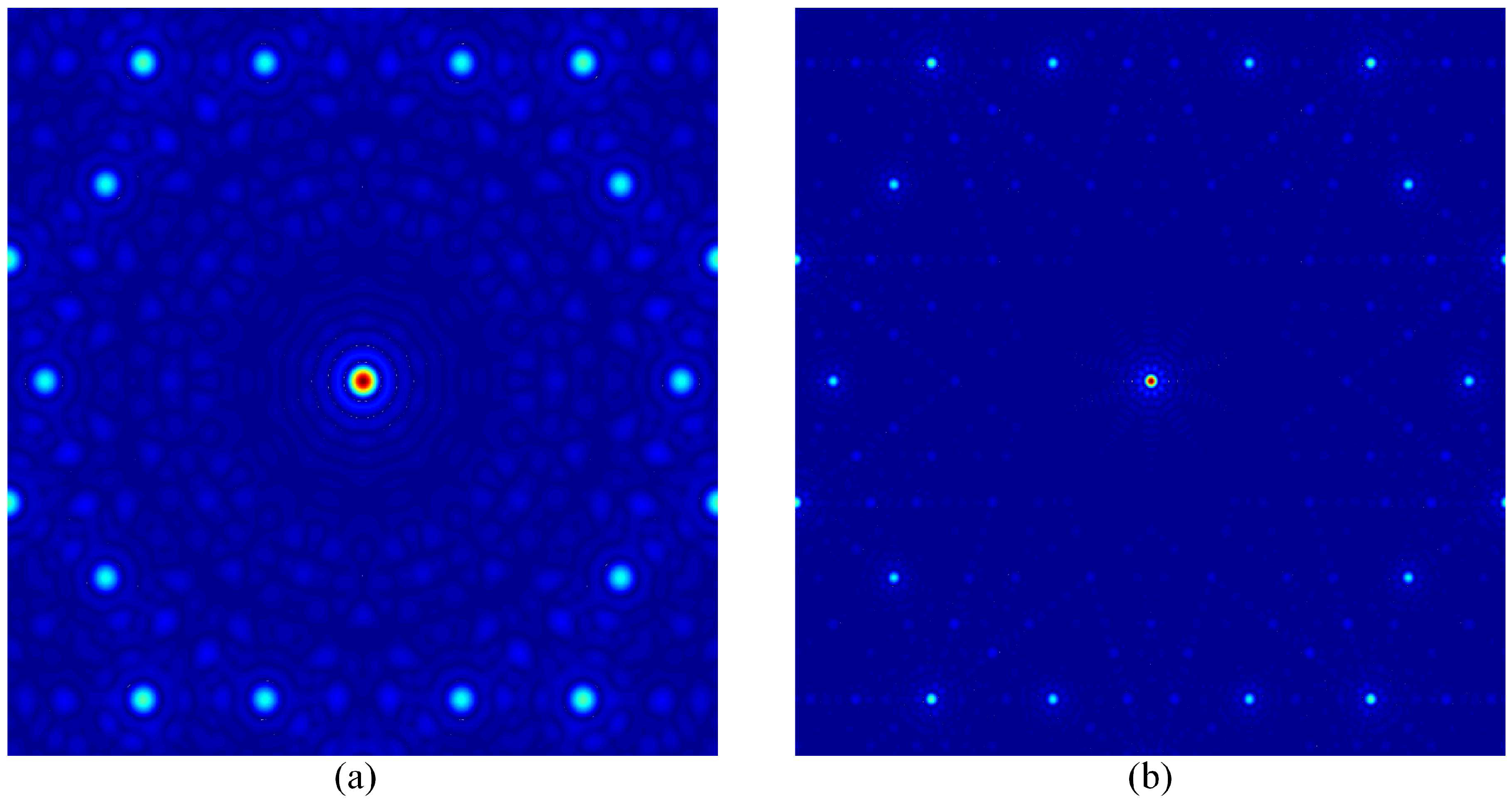
As noted earlier, a QC possess a discrete diffraction pattern. Figure 8a shows the magnitude of the normalized FT of a Penrose lattice with 731 points obtained from a Penrose tiling with prototile sides of $2{\tau }^2/\sqrt{5}$. Moreover, this prototile side corresponds to the lattice obtained by taking a 2D slice of the 4D hyper-lattice. As can be seen from Figure 8a, while there are several bright spots in the pattern, the pattern is not truly discrete, since there are ripples surrounding the bright spots. This is due to the finite size of the super-cell lattice. Figure 8b shows the magnitude of the normalized FT of a Penrose lattice with 1961 points. Compared to Figure 8a, the diffraction pattern in Figure 8b displays a much better discrete nature. However, while increasing the size of the super-lattice increases the accuracy of the diffraction pattern, it will also require much finer sampling in the reciprocal space since the diffraction peaks will become more delta-like with a very narrow width. Thus, a very fine sampling of the reciprocal space is required to capture all of the diffraction spots, which further increases the computational burden of the problem. The diffraction pattern in Figure 8b was obtained by sampling 3001 points along each dimension of the reciprocal space for a total of roughly nine million points.

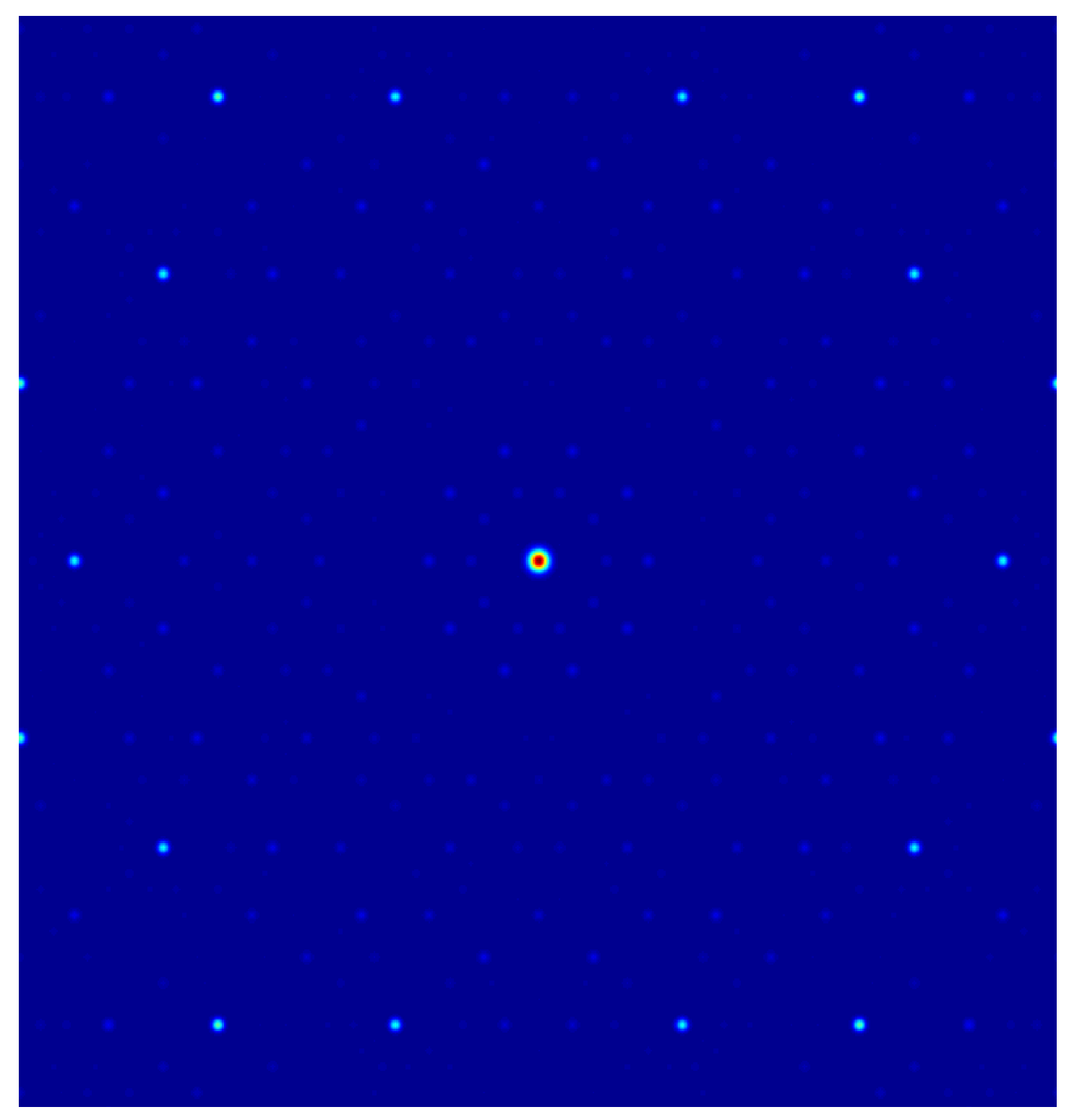
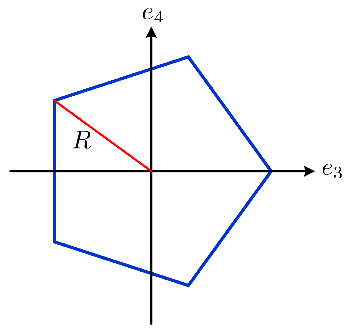
Figure 9 shows the normalized diffraction pattern of the Penrose QC obtained from the FS expansion of the 4D hyper-lattice with 279,841 terms $(N=11)$. Here, we note some important details regarding Figure 9. First, due to the very large number Fourier harmonics, we have performed a thresholding and only plotted Fourier harmonics above a certain threshold. We have used the threshold of $-40$ dB in Figure 9. Secondly, since it is extremely difficult to discern delta-like peaks in the diffraction pattern due to their infinitesimal width, to better visualize the discrete peaks, we have used Gaussian pulses of the form $A{e}^{\left(\alpha R^2\right)/A}$, where A is the amplitude of the Fourier harmonic expansion coefficient, R is the Euclidean distance from the location of the Fourier harmonic in the reciprocal space and α is some arbitrary positive decay constant.

Comparing Figure 8b with Figure 9, we can see that many of their features are identical. Both figures have been normalized, and as a result, it is difficult to discern peaks with a smaller magnitude. To overcome this issue, instead of plotting the normalized magnitude of the diffraction peaks, we plot the square root of the normalized magnitude. This non-linear mapping has the effect of enhancing smaller peaks, which allows for a better comparison of finer details. This comparison is illustrated in Figure 10. The square root of the normalized FS expansion harmonics obtained from the expansion of the ASs in the 4D hyper-lattice are displayed in Figure 10a, while Figure 10b plots the square root of the normalized FT of a Penrose super-lattice. As can be seen, these plots display many of the finer features not visible in Figure 8b and Figure 9. One of the most striking features seen in Figure 10a, which is not present in Figure 10b, is the discrete nature of the diffraction pattern. This phenomenon is particularly noticeable in the region surrounding the origin, where in Figure 10a, a series of discrete peaks are present, whereas in Figure 10b, a series of ripples surround the origin. The presence of ripples surrounding the bright spots in FT patterns can lead to inaccurate results in several ways. First, they can mask weaker diffraction peaks, as can be seen in Figure 10b, in the region surrounding the origin. Moreover, they also can lead to the appearance of spurious spots in the pattern (in-phase addition).

5. From the Vertex Model to Natural QCs

During our derivations, we assumed identical particles at all vertices. We call this the vertex model. This assumption is valid for many optical and photonic structures based on QC morphologies [12,14,16,17]. However, in natural QCs, this is not the case, and different atoms are placed at different vertices. Hence, an important question arises, which is, can this methodology be extended to natural QCs where the vertex model is no longer valid? Here, we show that our approach can be generalized to all types of QCs where ASs are decorated with different atoms.

To demonstrate the validity of our approach, let us consider the Penrose lattice with icosahedral symmetry. The Penrose lattice prototiles consist of a narrow rhombus tile (vertex angles $\pi /4$ and $4\pi /5$) shown in Figure 2a and a wide rhombus tile (vertex angles $2\pi /5$ and $3\pi /5$) shown in Figure 2b of identical sides. The tiling, shown in Figure 2c, is obtained by placing prototiles next to each other based on specific matching rules, which requires aligning arrows and double arrows. A close inspection of Figure 2c shows eight distinct types of vertices in the tiling denoted by ${}_1{}^{3}D$, ${}_2{}^{5}J$, ${}_4{}^{4}K$, ${}_1{}^{6}T$, ${}_2{}^{7}V$, ${}_5{}^{5}S$, ${}^{5}S$ and ${}_3{}^{3}Q$, as shown in Figure 11. For each vertex, the subscript corresponds to the number of double arrows surrounding it, and the superscript corresponds to the number of tiles surrounding it [28]. In fact, each of these vertices can be associated with a specific portion of the four pentagonal atomic surfaces, as shown in Figure 7. AS segments corresponding to each vertex type are shown in Figure 12, and the frequency of each vertex is directly proportional to its corresponding atomic surface [28].

In our vertex model, we assume identical particles at all vertices. Hence, to evaluate $c_{\mathbf{G}}$ in Equation (18), the integration was performed uniformly over all ASs. As noted before, this is valid for many optical and photonic structures based on QC morphologies; however, in natural QCs, this is not the case, and different atomic surfaces are decorated with different atoms. To account for different atoms at different vertices, the integration in Equation (18) must include a weighing factor for different regions of ASs corresponding to different vertices. While this has not been completely investigated, we believe that the weighing factor should be proportional to the mass of the atom occupying the atomic surface.

6. Conclusions

We have presented a rigorous method to obtain and analyze the diffraction properties of QC lattices. Previously, the diffraction patterns of QCs have been obtained by taking the FT of very large super-lattices. The first problem with using super-lattices is that they attempt to capture the properties of a QC by only considering a finite subset of an infinite structure. As a result, very large super-lattices are required to produce accurate results, which significantly increases the computational burden of the problem. Furthermore, as the size of the super-lattice is increased, the diffraction pattern becomes more discrete with delta-like peaks. Thus, the sampling in the reciprocal space must be performed with a very fine resolution to capture all of the diffraction spots.

Our method is based on the cut-and-project technique, which constructs QC lattices as lower dimensional slices of higher dimensional periodic hyper-lattices. The periodicity of the higher dimensional hyper-lattice makes it possible to expand the associated unit cell in terms of Fourier harmonics, which leads to a discrete spectrum. Unlike the super-lattice approach, our method is exact and captures all of the properties of the complete infinite QC structure.

The utility of the proposed method was demonstrated for two important QCs; the 1D Fibonacci and the 2D Penrose QCs. In both cases, we showed that it was possible to derive analytical expressions for the Fourier harmonics of the higher dimensional ASs. These findings were validated by comparing them to results obtained via the conventional approach based on evaluating the FT of very large hyper-lattices. Besides the large computational burden associated with applying a FT to super-lattices, we also demonstrated that such methods can lead to inaccurate results due to the continuous nature of the FT, which can generate spurious modes (due to the coherent addition of ripples) or null some modes (due to the destructive addition of ripples). Finally, we proposed how our approach can be generalized from the vertex model, which assumed identical particles at all vertices, to a more realistic case where different ASs are occupied by different atoms.

References

1. Senechal, M. Quasicrystals and Geometry; Cambridge University Press: Cambridge, UK, 1996. [Google Scholar]
2. Shechtman, D.; Blech, I.; Gratias, D.; Cahn, J.W. Metallic phase with long-range orientational order and no translational symmetry. Phys. Rev. Lett. 2013, 53, 1951–1953. [Google Scholar] [CrossRef]
3. Gopinath, A.; Boriskina, S.V.; Reinhard, B.M.; Negro, L.D. Deterministic aperiodic arrays of metal nanoparticles for surface-enhanced Raman scattering (SERS). Opt. Express 2009, 17, 3741–3753. [Google Scholar] [CrossRef] [PubMed]
4. Villa, A.D.; Galdi, V.; Capolino, F.; Pierro, V.; Enoch, S.; Tayeb, G. A comparative study of representative categories of EBG dielectric quasi-crystals. IEEE Antennas Wirelss Propagat. Lett. 2006, 5, 331–334. [Google Scholar] [CrossRef]
5. Wang, X.; Werner, D.; Turpin, J. Investigation of scattering properties of large-scale aperiodic tilings using a combination of the characteristic basis function and adaptive integral methods. IEEE Trans. Antenn. Propag. 2013, 61, 3149–3160. [Google Scholar] [CrossRef]
6. Mittra, R. (Ed.) Computational Electromagnetics: Recent Advances and Engineering Applications; Springer: New York, NY, USA, 2014; Chapter 12.
7. Spence, T.G.; Werner, D.H. Design of broadband planar arrays based on the optimization of aperiodic tilings. IEEE Trans. Antenn. Propag. 2008, 56, 76–86. [Google Scholar] [CrossRef]
8. Namin, F.; Petko, J.S.; Werner, D.H. Analysis and design optimization of robust aperiodic micro-UAV swarm-based antenna arrays. IEEE Trans. Antenn. Propag. 2012, 60, 2295–2308. [Google Scholar] [CrossRef]
9. Gross, F.B. (Ed.) Frontiers in Antennas: Next Generation Design & Engineering; McGraw-Hill: New York, NY, USA, 2011; Chapter 1.
10. Gopinath, A.; Boriskina, S.V.; Feng, N.; Reinhard, B.M.; Negro, L.D. Photonic-plasmonic scattering resonances in deterministic aperiodic structures. Nano Lett. 2008, 8, 2423–2431. [Google Scholar] [CrossRef] [PubMed]
11. Namin, F.; Wang, X.; Werner, D.H. Reflection and transmission coefficients for finite-sized aperiodic aggregates of spheres. J. Opt. Soc. Am. B 2013, 30, 1008–1016. [Google Scholar] [CrossRef]
12. Namin, F.A.; Yuwen, Y.A.; Liu, L.; Panaretos, A.H.; Werner, D.H.; Mayer, T.S. Efficient design , accurate fabrication and effective characterization of plasmonic quasi-crystalline arrays of nano- spherical particles 2016. Sci. Rep. 2016, 6, 22009. [Google Scholar] [CrossRef] [PubMed]
13. Pala, R.A.; White, J.; Barnard, E.; Liu, J.; Brongersma, M.L. Design of plasmonic thin-film solar cells with broadband absorption enhancements. Adv. Mat. 2009, 21, 3504–3509. [Google Scholar] [CrossRef]
14. Bauer, C.; Kobiela, G.; Giessen, H. 2D quasiperiodic plasmonic crystals. Sci. Rep. 2012, 2, 681. [Google Scholar] [CrossRef] [PubMed]
15. Kaliteevski, M.A.; Brand, S.; Abram, R.A.; Krauss, T.F.; Millar, P.; Rue, R.M.D.L. Diffraction and transmission of light in low-refractive index Penrose-tiled photonic quasicrystals. J. Phys. Condens. Matter 2001, 13, 10459–10470. [Google Scholar] [CrossRef]
16. Matsui, T.; Agrawal, A.; Nahata, A.; Vardeny, Z.V. Transmission resonances through aperiodic arrays of subwavelength apertures. Nature 2007, 446, 517–521. [Google Scholar] [CrossRef] [PubMed]
17. Agrawal, A.; Matsui, T.; Vardeny, Z.V.; Nahata, A. Terahertz transmission properties of quasiperiodic and aperiodic aperture arrays. J. Opt. Soc. Am. B 2007, 24, 2545–2555. [Google Scholar] [CrossRef]
18. Steurer, W.; Deloudi, S. Crystallography of Quasicrystals: Concepts, Methods and Structures; Springer: Berlin, Germany, 2009. [Google Scholar]
19. Achanta, V.G. Plasmonic quasicrystals. Prog. Quant. Electron. 2015, 39, 1–23. [Google Scholar] [CrossRef]
20. Janssen, T.; Chapuis, G.; de Boissieu, M. Aperiodic Crystals: From Modulated Phases to Quasicrystals; Oxford University Press: Oxford, UK, 2007. [Google Scholar]
21. Baake, M.; Kramer, P.; Schlottmann, M.; Zeidler, D. Planar patterns with fivefold symmetry as sections of periodic structures in 4-space. Int. J. Mod. Phys. B 1990, 04, 2217–2268. [Google Scholar] [CrossRef]
22. Penrose, R. The role of aesthetics in pure and applied mathematical research. Inst. Math. Appl. Bull. 1974, 10, 266–271. [Google Scholar]
23. Yamamoto, A.; Hiraga, K. Structure of an icosahedral Al-Mn quasicrystal. Phys. Rev. B 1988, 37, 6207. [Google Scholar] [CrossRef]
24. Ishihara, K.N.; Yamamoto, A. Penrose patterns and related structures. I. Superstructure and generalized Penrose patterns. Acta Crystallogr. Sect. A 1988, 44, 508–516. [Google Scholar] [CrossRef]
25. Rodriguez, A.W.; McCauley, A.P.; Avniel, Y.; Johnson, S.G. Computation and visualization of photonic quasicrystal spectra via Bloch’s theorem. Phys. Rev. B 2008, 77, 104201. [Google Scholar] [CrossRef]
26. Namin, F.A.; Werner, D.H. Rigorous analysis of diffraction from quasicrystalline gratings via Floquet’s theorem in higher-dimensional space. ACS Photonics 2014, 1, 212–220. [Google Scholar] [CrossRef]
27. Dubois, J. Useful Quasicrystals; World Scientific: Hackensack, NJ, USA, 2005. [Google Scholar]
28. Pavlovitch, A.; Kléman, M. Generalised 2D Penrose tilings: structural properties. J. Phys. A 1987, 20, 687. [Google Scholar] [CrossRef]
Figure 1. Normalized FT (magnitude) of a Fibonacci lattice with 4181 points. The reciprocal space region 10 s 10 has been sampled at 100,001 points.
Crystals 06 00093 g001
Figure 2. (a) The narrow prototile (vertex angles π / 4 and 4 π / 5 ) and (b) the wide prototile (vertex angles 2 π / 5 and 3 π / 5 ) of the Penrose tiling; (c) the tiling obtained based on specific matching rules, which requires aligning arrows and double arrows, while placing prototiles next to each other.
Crystals 06 00093 g002
Figure 3. The normalized FT (magnitude) of the Penrose point lattice.
Crystals 06 00093 g003
Figure 4. 2D embedding of the Fibonacci quasicrystal (QC) showing (a) the selection window for the 2D hyper-lattice projection and (b) the decorated hyper-lattice of a Fibonacci QC with atomic surfaces (ASs) of length Δ.
Crystals 06 00093 g004
Figure 5. Diffraction pattern of the Fibonacci QC obtained by Fourier series (FS) expansion of the higher dimensional unit cell, as shown in Figure 4b. Fourier harmonics (magnitude) are plotted versus the parallel component of the corresponding reciprocal vectors (RVs).
Crystals 06 00093 g005
Figure 6. Normalized FT (magnitude) of a Fibonacci lattice with 2585 points. The reciprocal space region 10 s 10 has been sampled at 10,001 points in (a) and at 20,001 points in (b).
Crystals 06 00093 g006
Figure 7. Projection of 4D hyper-rhombohedral unit cell onto the perpendicular space E . The four ASs have been highlighted, and the perpendicular space basis vectors e ^ 3 and e ^ 4 have been shown for reference.
Crystals 06 00093 g007
Figure 8. Normalized FT (magnitude) of a Penrose lattice with 371 points in (a) and with 1961 points in (b).
Crystals 06 00093 g008
Figure 9. Diffraction pattern of the Penrose QC obtained from the FS expansion of a 4D hyper-lattice with 2 × 11 + 1 4 = 279,841 terms. The magnitude of the Fourier harmonics is plotted versus the parallel space component of the RVs.
Crystals 06 00093 g009
Figure 10. (a) Square root of the normalized FS harmonics (magnitude) of the Penrose QC obtained using the expansion of the 4D hyper-lattice; (b) square root of the normalized FT (magnitude) of a Penrose super-lattice.
Crystals 06 00093 g010
Figure 11. Eight distinct types of vertices in the Penrose tiling, as shown in Figure 2c, denoted by D 1 3 , J 2 3 , K 4 4 , T 1 6 , V 2 7 , S 5 5 , S 5 and Q 3 3 .
Crystals 06 00093 g011
Figure 12. (a) The portions of atomic surface D corresponding to vertices D 1 3 , S 5 , K 4 4 ; (b) portions of atomic surface C corresponding to vertices Q 3 3 , J 2 5 , T 1 6 , V 2 7 and S 5 . Those in B and A are related by an inversion center.
Crystals 06 00093 g012