Article

Second-Harmonic Generation in Membrane-Type Nonlinear Acoustic Metamaterials

by
Jiangyi Zhang
1,
Vicente Romero-García
1,
Georgios Theocharis
1,
Olivier Richoux
1,*,
Vassos Achilleos
1 and
Dimitris J. Frantzeskakis
2
1
LUNAM Université, Université du Maine, CNRS, LAUM UMR 6613, Av. O. Messiaen, Le Mans 72085, France
2
Department of Physics, National and Kapodistrian University of Athens, Panepistimiopolis, Zografos, Athens 15784, Greece
*
Author to whom correspondence should be addressed.
Crystals 2016, 6(8), 86; https://doi.org/10.3390/cryst6080086
Submission received: 11 April 2016 / Revised: 21 July 2016 / Accepted: 25 July 2016 / Published: 29 July 2016
(This article belongs to the Special Issue Phononic Crystals)

Abstract

:
We study analytically and numerically the second-harmonic generation in a one-dimensional nonlinear acoustic metamaterial, composed of an air-filled waveguide periodically loaded by clamped elastic plates. Based on the transmission line approach, we derive a nonlinear dynamical lattice model which, in the continuum approximation, leads to a nonlinear dispersive wave equation. By applying the perturbation method to the latter, we derive the analytical expressions for the first- and second-harmonics, which are in excellent agreement with the numerical simulations of the nonlinear dynamical lattice model. Apart from the case of dispersionless nonlinear propagation and the Fubini solution, special attention is payed to the role of dispersion. In that regard, it is found that, once dispersion comes into play, second-harmonic beatings in space due to phase-mismatch can be identified. Our results provide many opportunities for the development of new periodic acoustic structures featuring both nonlinearity and dispersion.

Graphical Abstract

1. Introduction

Phononic crystals and acoustic metamaterials have been widely popularized since the beginning of the 21st century because of the exotic properties they offer, including subwavelength focusing, cloaking, and extraordinary transmission among others [1]. These materials are composite structures designed to tailor acoustic wave dispersion through Bragg’s scattering and local resonances. One of the main properties of the phononic crystals and acoustic metamaterials is that—thanks to their periodic structure—they exhibit phononic band gaps, namely ranges of frequencies where no propagation occurs (i.e., linear acoustic waves are evanescent). The existence of band gaps has been studied in theory and observed experimentally for the first time in periodic acoustic waveguides by Sugimoto [2] and Bradley [3]. In 2000, Liu et al. [4] paved the way to acoustic metamaterials through phononic crystals that exhibited spectral gaps with lattice constants two orders of magnitude smaller than the relevant acoustic wavelength. The formation of band gaps in these acoustic metamaterials is based on the idea of the inclusion of locally resonant structures. These, in turn, usually determine the properties of acoustic metamaterials, rather than their composition.
Most of the works in the field of phononic crystals and acoustic metamaterials are restricted in the linear regime, and they do not consider the nonlinearity of the medium. Nevertheless, as the amplitude of the wave excitation is increased, the response of the metamaterial becomes nonlinear. This may give rise to different phenomena including, for instance, harmonic generation [5,6] and emergence of solitons [7], namely robust localized waves propagating undistortedly due to a balance between dispersion and nonlinearity. Nonlinear acoustic metamaterials are very good candidates to analyze the combined effects of nonlinearity and dispersion, occurring, e.g., in the beating of higher generated harmonics, because of mismatched phases or the existence of solitons [8,9].
In the context of electromagnetic (EM) metamaterials, there exist many works devoted to the nonlinear behavior [10,11,12,13,14]. Typically, metamaterials can be realized or modeled by a quasi-lumped transmission line (TL), with elementary cells consisting of a series inductor and a shunt capacitor, the dimensions of which are much less than the wavelength of the operating frequency. The TL approach is a powerful tool for studying nonlinear phenomena in EM metamaterials, such as soliton formation and nonlinear propagation [11,12,13,14]. In the context of acoustic metamaterials, one may similarly employ an acoustic circuit modeling, in which the voltage corresponds to the acoustic pressure and the current to the volume velocity flowing through the waveguide, in order to characterize the nonlinear propagation. On the other hand, the linear TL description of acoustic metamaterials has gained considerable attention the last few years [15,16,17,18,19]. However, studies on nonlinear phenomena in such settings are rather limited [9].
In this work, we consider an acoustic metamaterial composed of an air-filled waveguide, periodically side-loaded by clamped elastic plates. For such a system, it is well known that the elastic plates are incorporated as resonant elements and are considered to be in series in the electro-acoustic analogy [15,16,17,18,19]. Nonlinear wave propagation in this dispersive structure is theoretically and numerically studied. The paper is structured as follows. Based on the nonlinear transmission line theory, in Section 2, we introduce the 1D nonlinear lattice model, and employing the continuum approximation, we derive the nonlinear dispersive wave equation. Linear and nonlinear properties of the model, namely the dispersion relation and the case of dispersionless nonlinear propagation, are respectively studied in Section 3 and Section 4. In Section 5, by applying a perturbation method, we study the second-harmonic generation, while the effect of dispersion is studied in detail in Section 6. Finally, in Section 7, we present our conclusions and discuss future research directions.

2. Electro-Acoustic Analogue Modeling

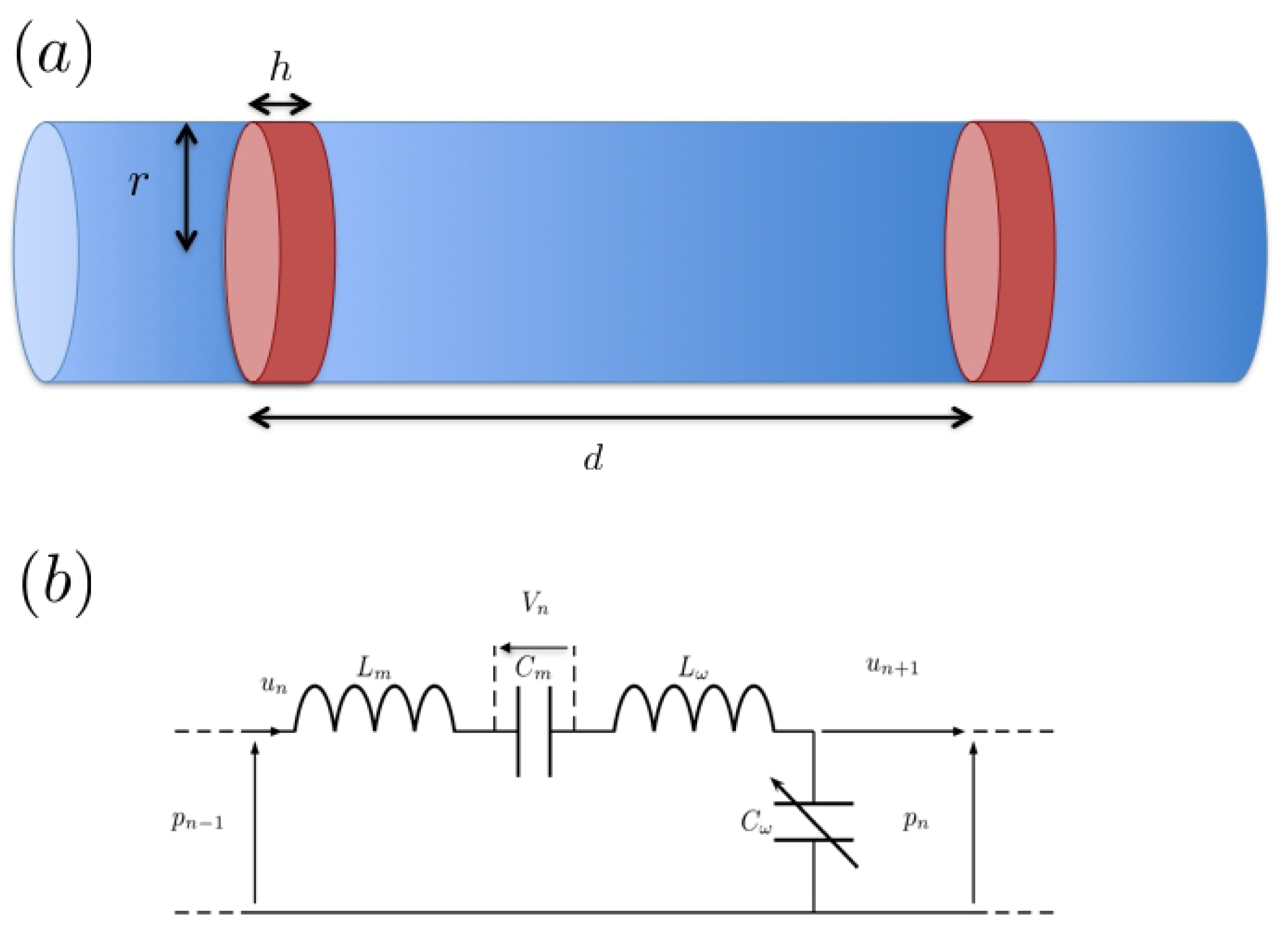
We consider low-frequency wave propagation in an acoustic waveguide periodically loaded with elastic plates. The frequency range considered is well below the first cut-off frequency of the higher propagative modes in the waveguide, therefore the problem is considered as one-dimensional. The distance between the plates is d and the plates have a thickness h and radius r, as shown in Figure 1a.
In order to theoretically analyze this system, in this work, we adopt the electro-acoustic analogy. Using physical acoustics, one has to treat our setting by solving two nonlinear partial differential equations for the pressure and velocity field coupled at specific points (where the resonators are located) with a number of ordinary differential equations that describe the dynamics of the resonators (in our case the clamped elastic plates). This kind of modeling is very hard to treat analytically and one has only to rely on numerical simulations. On the contrary, one could use the electro-acoustical analogy to derive a nonlinear discrete wave equation, describing wave propagation in an equivalent electrical transmission line, which can be solved perturbatively in the continuum limit. Such an approach provides an efficient way to treat the nonlinearity and greatly simplifies the problem, allowing for straightforward analytical treatment by means of standard techniques that are used in other physical systems. Then, in this work, the voltage v and the current i of the equivalent electrical transmission line corresponds to the acoustic pressure p and to the volume velocity u flowing through the waveguide cross-section, respectively.
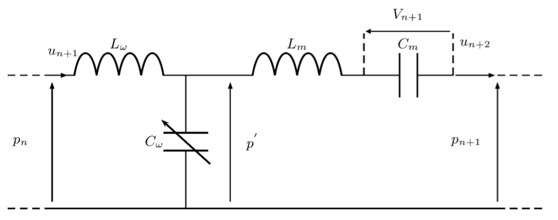
Following the TL approach, we start our consideration with the unit-cell circuit of the equivalent TL model of this setting. There are two different forms for the unit-cell circuit, as shown in Figure 1b and Figure A1 (see Appendix). Here, we only introduce the first one. The other circuit is introduced in the Appendix [18,19].
The unit-cell is composed of two parts, one corresponding to the propagation in the tube and the other one to the elastic plate. The resonant elastic plate can be modeled by an L C circuit, namely the series combination of an inductance L m and a capacitance C m , given by
L m = ρ m h S , C m = 1 ω m 2 L m ,
where ρ m is the plate density, S represents the cross-section area of the plate, while ω m = 2 π f m is the resonance frequency of the plate, with
f m = 0 . 4694 h r 2 E ρ m ( 1 ν 2 ) ,
where r is the radius of the elastic plate, E is the Young’s modulus and ν is the Poisson ratio [18,19]. We consider elastic plates made of rubber, with ρ m = 1420 kg/m 3 , E = 2 . 758 GPa and ν = 0 . 34 . The part of the unit-cell circuit that corresponds to the waveguide is modeled by the inductance L ω and shunt capacitance C ω ; the linear parts of these elements are given by
L ω 0 = ρ 0 d S , C ω 0 = S d ρ 0 c 0 2 ,
where ρ 0 and c 0 are, respectively, the density and the sound velocity of the fluid in the waveguide that has a cross section S = π r 2 .
In this work, we consider the response of the elastic plate to be linear and the propagation in the waveguide weakly nonlinear. This is a reasonable approximation, since the amplitudes used in this work are not sufficient to excite nonlinear vibrations of the elastic plate [9,20]. Due to the compressibility of the air, the wave celerity is a nonlinear term, c N L . Thus, we consider that the capacitance C ω is nonlinear and depends on the pressure p. Approximating the celerity as c N L c 0 1 + β 0 p / ρ 0 c 0 2 , where β 0 is the nonlinear parameter for the case of air (that is β 0 = 1 . 2 ), the pressure-dependent capacitance C ω can be expressed as
C ω = C ω 0 C ω p n ,
C ω = 2 β 0 ρ 0 c 0 2 C ω 0 .
The inductance remains in the same form as in the linear part, L ω 0 = L ω . Next, we will derive an evolution equation for the pressure in the n-th cell of the lattice as follows.
First, we note that the advantage of the considered unit-cell circuit is that the inductances L ω and L m are in a series connection and, thus, can be substituted by the inductance L = L ω + L m (see Figure 1b). Applying Kirchoff’s voltage law for two successive cells yields
p n 1 p n = L d d t u n + V n ,
p n p n + 1 = L d d t u n + 1 + V n + 1 ,
where V n is the voltage produced by the capacitance of the elastic plates C m . Subtracting the two equations above, we obtain the differential-difference equation (DDE)
δ ^ 2 p n = L d d t u n u n + 1 + V n V n + 1 ,
where δ ^ 2 p n p n + 1 2 p n + p n 1 . Then, Kirchhoff’s current law yields
u n u n + 1 = C ω d d t p n ,
with
u n = C m d d t V n and u n + 1 = C m d d t V n + 1 .
Subtracting Equation (10) and employing Equation (9), we obtain
u n u n + 1 = C m d d t V n V n + 1 = C ω d d t p n .
Then, recalling that the capacitance C ω depends on the pressure (cf. Equation (4)), we express V n V n + 1 as
V n V n + 1 = C ω C m p n = C ω 0 C m p n C ω C m p n 2 .
Next, substituting Equations (9) and (12) into Equation (8), we obtain the following evolution equation for the pressure
δ ^ 2 p n = L d d t C ω d d t p n + C ω 0 C m p n C ω C m p n 2 .
To this end, employing Equation (4), we can rewrite the above equation as follows:
δ ^ 2 p n L C ω 0 d 2 p n d t 2 C ω 0 C m p n + L C ω 2 d 2 p n 2 d t 2 + C ω C m p n 2 = 0 .
In this article, we have numerically integrated the nonlinear lattice model, Equation (14), by using the function ode45 of Matlab which is based on the Runge Kutta method, with an initial condition, p 1 = sin ( ω t ) at x = 0 , where ω = 2 π f is the angular frequency of the driver. For each simulation, we ensure the validity of the Courant–Friedrichs–Lewy (CFL) condition, c d t d x 1 , where c is the phase velocity, d t and d x are the time step and length interval, respectively. We also pay attention to the length of the system, which should be long enough to avoid reflections in the analyzed signal.

2.1. The Continuum Approximation

For our analytical considerations, we will focus on the continuum limit of Equation (14), corresponding to n and d 0 (but with n d being finite); in such a case, the pressure becomes p n ( t ) p ( x , t ) , where x = n d is a continuous variable, and
p n ± 1 = p ± d p x + d 2 2 2 p x 2 ± d 3 3 ! 3 p x 3 + d 4 4 ! 4 p x 4 + O ( d 5 ) ,
i.e., the difference operator δ ^ 2 is approximated by δ ^ 2 p n d 2 p x x + d 4 12 p x x x x . Keeping the O ( d 4 ) derivative term, the PDE contains also the weak dispersion that originates from the periodicity of the elastic plates array as we will see later on. Terms of the order O ( d 5 ) and higher are neglected, and subscripts denote partial derivatives. This way, Equation (14), becomes the following PDE:
d 2 p x x + d 4 12 p x x x x L C ω 0 p t t C ω 0 C m p + 1 2 L C ω p 2 t t + C ω C m p 2 = 0 .
It is also convenient to express our model in dimensionless form; this can be done upon introducing the normalized variables τ and χ and normalized pressure p, which are defined as follows: τ is time in units of ω B 1 , where ω B = π c 0 / d is the Bragg frequency; χ is space in units of c / ω B , where the velocity is given by
c = c 0 1 + α , α = h ρ m d ρ 0 ,
and p is pressure in units of p 0 = ρ 0 c 0 2 . Then, Equation (16) is reduced to the following dimensionless form:
p τ τ p χ χ γ p χ χ χ χ + m 2 p = 2 β 0 m 2 p 2 + β 0 p 2 τ τ ,
where parameters m 2 and γ are given by
m 2 = α 1 + α ω m ω B 2 , γ = 1 12 π 2 ( 1 + α ) .
It is interesting to identify various limiting cases of Equation (18). First, in the linear limit ( β 0 = 0 , or p 2 1 ) , and in the absence of plates ( m 2 0 , and without considering higher order spatial derivatives), Equation (18) is reduced to the linear wave equation, p τ τ p χ χ = 0 . In the linear limit, in the presence of plates and in the long wavelength approximation ( k 0 , and without considering higher order spatial derivatives), Equation (18) takes the form of the linear Klein–Gordon equation [7], p τ τ p χ χ + m 2 p = 0 , with the parameter m playing the role of mass. Finally, in the nonlinear regime, but when plates are absent, Equation (18) is reduced to the well-known Westervelt equation, p τ τ p χ χ β 0 p 2 τ τ = 0 , which is a common nonlinear model describing 1D acoustic wave propagation [21].

3. The Linear Dispersion Relation

We now consider the linear limit of Equation (18) and the respective dispersion relation. Assuming propagation of plane waves, of the form p e x p [ i ( k χ ω τ ) ] , we obtain the following dispersion relation connecting the wavenumber k and frequency ω
D ( ω , k ) = ω 2 + k 2 γ k 4 + m 2 = 0 .
For D ( ω , k ) = 0 , this is the familiar dispersion relation of the linear Klein–Gordon model. It is clear that Equation (20) suggests the existence of a gap at low frequencies, i.e., for 0 ω < m , with the cut-off frequency defined by the parameter m. For m < ω < ω B , there exists a band, with the dispersion curve ω ( k ) having the form of hyperbola, which asymptotes (according to Equation (20)) to unity, which is the normalized velocity associated with the wave equation p τ τ p χ χ = 0 . The term γ k 4 accounts for the influence of the periodicity of the lattice (originating from the term δ ^ 2 p n ) to the dispersion relation. Although this term appears to lead to instabilities for large values of k, both Equations (18) and (20) are used in our analysis only in the long wavelength limit where k is sufficiently small.
Since all quantities in the above dispersion relation are dimensionless, it is also relevant to express it in physical units. In particular, taking into account that the frequency ω p h and wavenumber k p h in physical units are connected with their dimensionless counterparts through ω = ω p h / ω B and k = k p h c ω B , we can express Equation (20) in the following form:
ω p h 2 + k p h 2 c 2 γ k p h 4 c 4 ω B 2 + m 2 ω B 2 = 0 .
Solving Equation (21) analytically with respect to k p h , we can then determine the frequency f = ω p h / 2 π as a function of the wavenumber k p h 
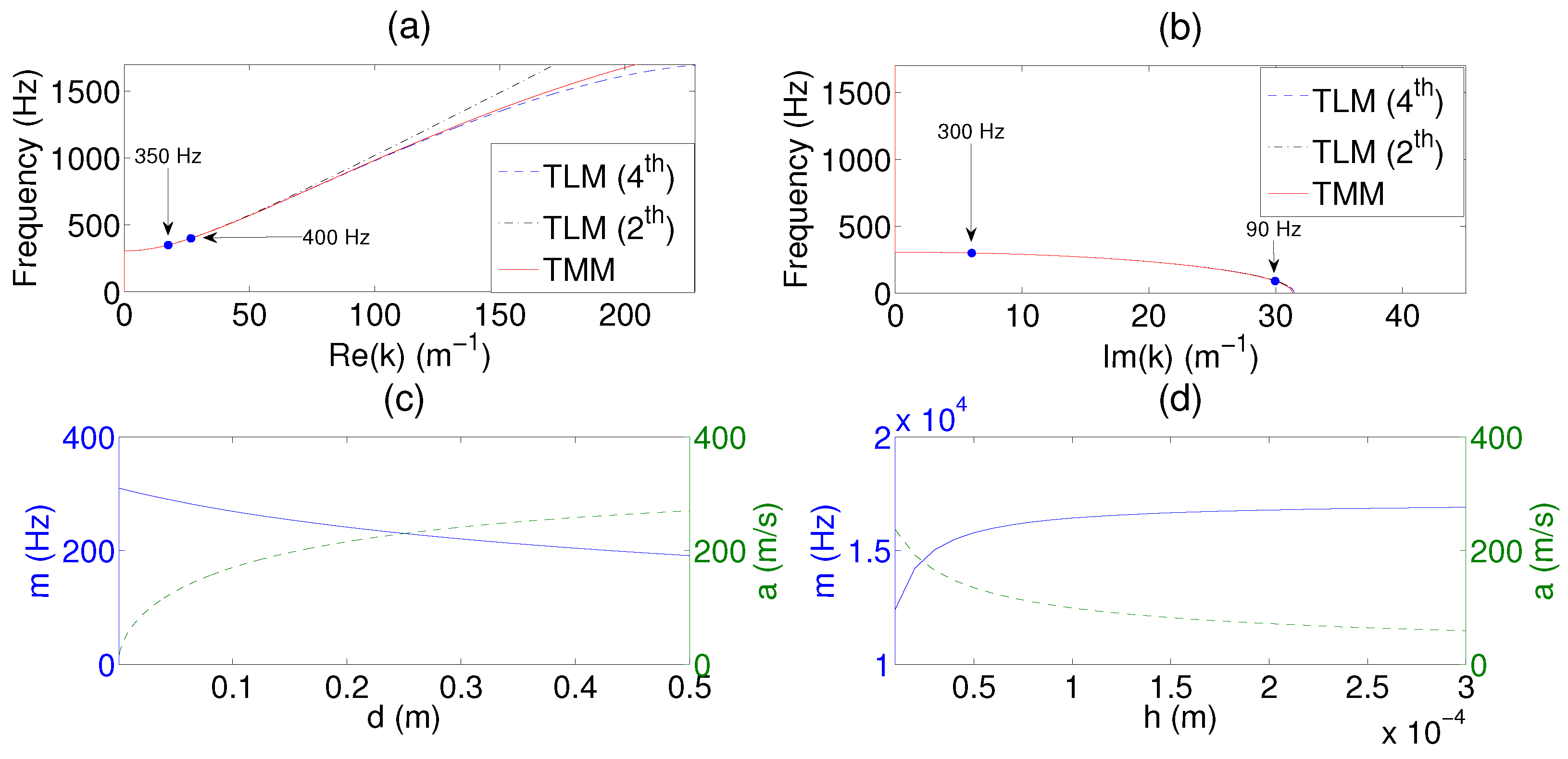
, and plot the resulting dispersion relation. The real and imaginary parts of the dispersion relation are respectively plotted in Figure 2a,b for a metamaterial composed of elastic plates made of rubber with thickness h = 2 . 78 × 10 4 m and with a periodicity d = 0 . 01 m. The dispersion relation features the band gap from 0 Hz to m ω B 2 π Hz due to the combined effect of the resonance of the plate and of the geometry of the system. The upper limit of this band gap is found to be sufficiently smaller than the Bragg band frequency f B = c 0 / 2 d = 17163 Hz, with c 0 = 343 . 26 m/s. The propagating band has two parts: a strongly dispersive and a weakly dispersive one. In the lower weakly dispersive region, there is a “quasi-linear” dispersion with the slope a = c 0 1 + α (which is identical to the velocity c in Equation (17)), and the upper weakly dispersive region is due to the periodicity of lattice. Both the periodicity of the system d and the thickness of the elastic plates could influence the first cut-off frequency m and the slope a of the “quasi-linear” dispersion, as shown in the Figure 2c,d. The first cut-off frequency m is inversely proportional to the periodicity of the lattice d and proportional to the thickness of the elastic plates h, while the slope a of the “quasi-linear” dispersion increases with the increase of d and the decrease of h. Due to periodicity, the band structure of our system exhibits a Bragg band gap with an upper edge k d = π located at 17 . 163 kHz. The lower edge of the gap, however, also depends on α (describing the impedance mismatch and the filling fraction) and is located much lower at 1 . 988 kHz. Due to the dispersion around this lower band gap edge, the 4th order spatial derivative term is needed to describe the system in a good accuracy. To further illustrate the importance of the higher order dispersive term, in Figure 2a we additionally show a curve corresponding to the case without it ( γ = 0 ).
On the other hand, the red lines in the Figure 2a,b show the respective results (for the lossless case under consideration) for the dispersion relation, as obtained using the transfer matrix method (TMM) [3]
cos ( k p h d ) = cos ( ω p h c 0 d ) + i Z m 2 Z 0 sin ( ω p h c 0 d ) ,
where Z m = i ω p h L m 1 / ω p h C m is the impedance of the plate for the lossless case in the long wavelength approximation, and Z 0 = ρ 0 c 0 / S the acoustic characteristic impedance of the waveguide. Comparing the dispersion relation obtained by using TMM, with the one resulting from the continuum approximation, Figure 2a,b, we find an excellent agreement between these two in the regime of low frequencies, namely sufficiently lower to the Bragg frequency.

4. Dispersionless Nonlinear Propagation

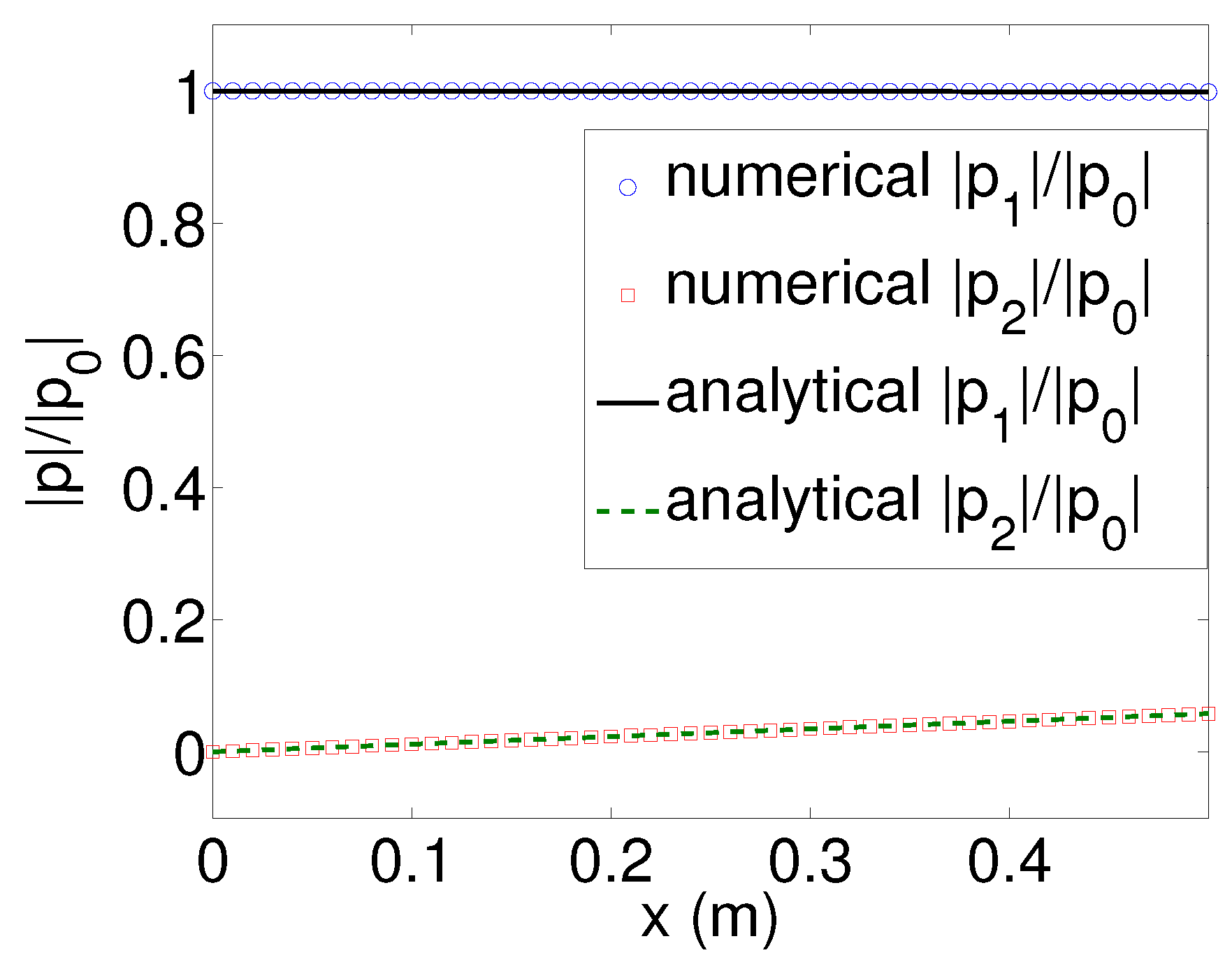
We now consider the nonlinear regime, without dispersion due to the periodicity of the lattice and the resonance of the plates, i.e., the well-known Westervelt equation. As the large-amplitude wave propagates, the amplitude of the fundamental component | p 1 | will decrease continuously as the energy is transferred to the nonlinearly generated higher-harmonic components ( | p 2 | , etc. ). The growth of the higher harmonics is displayed in the pre-shock region which is defined by σ 1 , where σ = x / x s h is a dimensionless shock formation distance. The shock distance,
x s h = ρ c 3 2 π f β p 0 ,
is proportional to the velocity and inversely proportional to the pressure amplitude and source frequency for a fixed medium. Here, the source condition is p ( 0 , t ) = p 0 sin ω t , where p 0 = 0 . 04 P 0 (with P 0 being the atmospheric pressure), and sin ω t is periodic in time with fundamental frequency f = 400 Hz. If this initial state propagates in a dispersionless waveguide—cf. Figure 3—its shock distance will be around 4 m. In the near source region, the pertinent Fubini solution has certain asymptotic properties [21]. The amplitude of the second harmonic component increases linearly to the propagation distance:
| p 1 | / | p 0 | = 1 1 8 σ 2 + O ( σ 4 ) ,
| p 2 | / | p 0 | = 1 2 σ + O ( σ 3 ) .
As shown in Figure 3, the numerical results (circles) are in a good agreement with the Fubini solution (solid lines).

5. Combining Dispersion and Nonlinearity: Perturbation Method

Now, we study the second-harmonic generation in the presence of the periodic array of the elastic plates, namely in the presence of dispersion. Our analysis relies on the determination of approximate solutions of Equation (18) by using a perturbative approach.
We now express p as an asymptotic series in ϵ
p = ϵ p 1 + ϵ 2 p 2 + ϵ 3 p 3 + ,
where 0 < ϵ 1 is a formal small parameter. Here, the introduced ϵ is the acoustic Mach number, defined as ϵ = p 0 ρ c 2 , where p 0 is the amplitude of the incident wave. Then, substituting Equation (26) into Equation (18), we obtain a hierarchy of equations at various orders in ϵ. Of particular importance in our analysis are the equations at the first two orders, which are as follows.
At the leading order, O ( ϵ 1 ) , the resulting equation is
2 p 1 τ 2 2 p 1 χ 2 γ 4 p 1 χ 4 + m 2 p 1 = 0 ,
which possesses plane wave solution of the form
p 1 = 1 2 exp ( i θ ) + c . c . cos ( θ ) ,
where c.c. denotes complex conjugate, θ = ω τ k ( ω ) χ is the phase, while parameters k and ω satisfy the dispersion relation Equation (20). Next, we consider the equation at the order O ( ϵ 2 ) ,
2 p 2 τ 2 2 p 2 χ 2 γ 4 p 2 χ 4 + m 2 p 2 = 2 β 0 m 2 p 1 2 + β 0 2 p 1 2 τ 2 .
Substituting Equation (28) into Equation (29), and using the identity cos 2 ( θ ) = cos ( 2 θ ) + 1 / 2 , we rewrite Equation (29) as follows:
2 p 2 τ 2 2 p 2 χ 2 γ 4 p 2 χ 4 + m 2 p 2 = m 2 2 ω 2 β 0 cos 2 θ .
The solution of this equation is the sum of the general solution p 2 h of the homogeneous equation and the particular solution p 2 p of the inhomogeneous equation, namely p 2 = p 2 h + p 2 p , where the corresponding waves for these two solutions are the free and forced waves respectively; these solutions read
p 2 h = p 2 h ( x = 0 ) cos ( 2 ϕ ) = 1 2 p 2 h ( x = 0 ) exp ( i 2 ϕ ) + c . c . ,
p 2 p = m 2 2 ω 2 D ( 2 ω , 2 k ) β 0 cos 2 θ = 1 2 m 2 2 ω 2 D ( 2 ω , 2 k ) β 0 exp ( i 2 θ ) + c . c . ,
where 2 ϕ = 2 ω τ k ( 2 ω ) χ , and k ( 2 ω ) is the wavenumber of the free wave at second harmonic frequency. As long as 2 k ( ω ) k ( 2 ω ) , which is the case in dispersive media, the forced and free waves have different phase speeds, i.e., they are phase-mismatched. Since there is no second harmonic at x = 0 , we can set
p 2 h ( x = 0 ) = m 2 2 ω 2 D ( 2 ω , 2 k ) β 0 .
Thus, the evolution of the second harmonic field p 2 can directly be found as a combination of Equations (32) and (31):
p 2 = 2 m 2 2 ω 2 D ( 2 ω , 2 k ) β 0 sin Δ k 2 χ sin ( 2 ω τ k eff χ ) ,
where k eff is the effective wave number,
k eff = 2 k ( ω ) + k ( 2 ω ) / 2 ,
while Δ k is the detuning parameter that describes the asynchronous second harmonic generation,
Δ k = k ( 2 ω ) 2 k ( ω ) = k 2 2 k 1 .
Obviously, in the linear limit ( β 0 = 0 ), p 2 
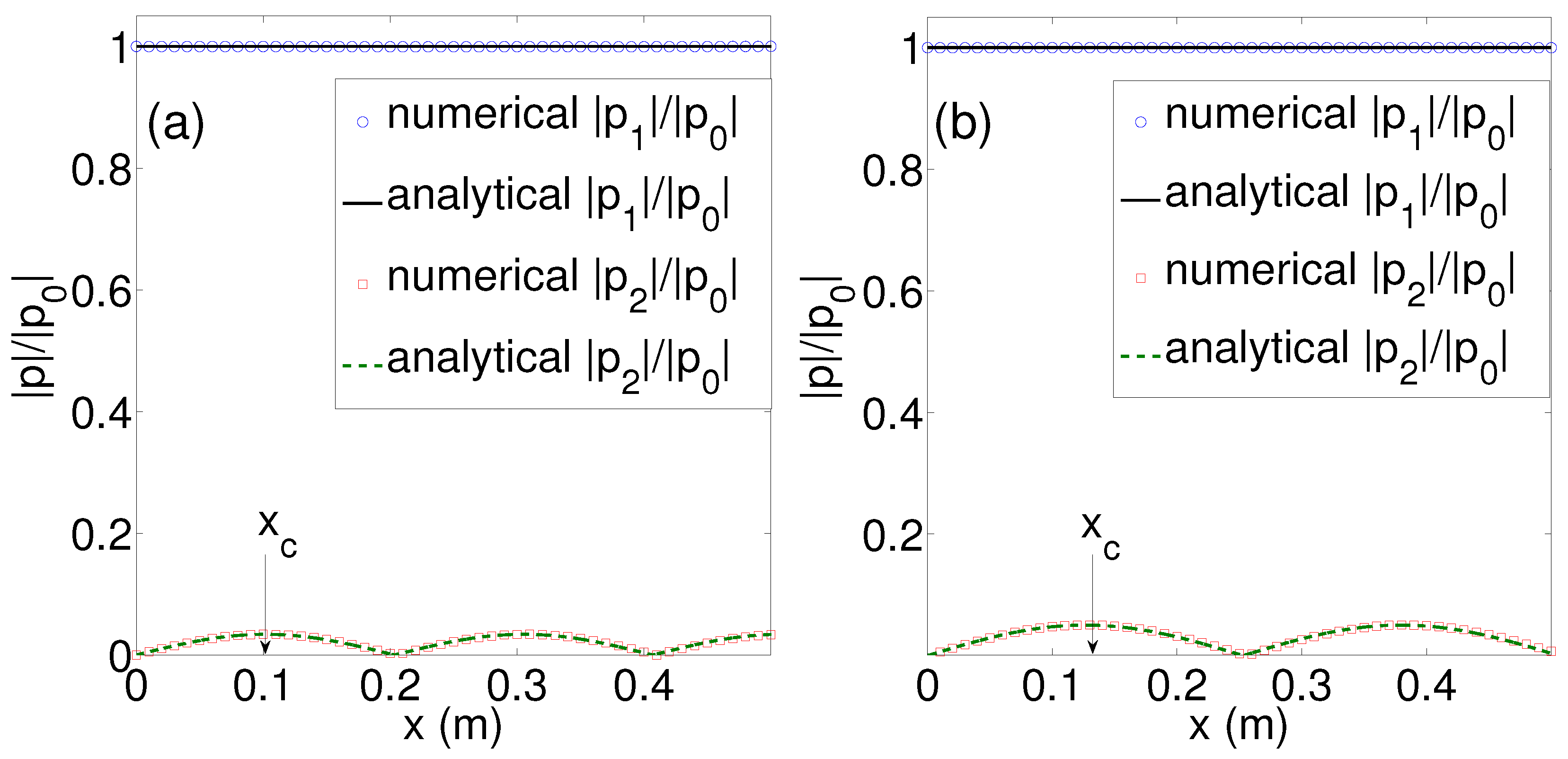
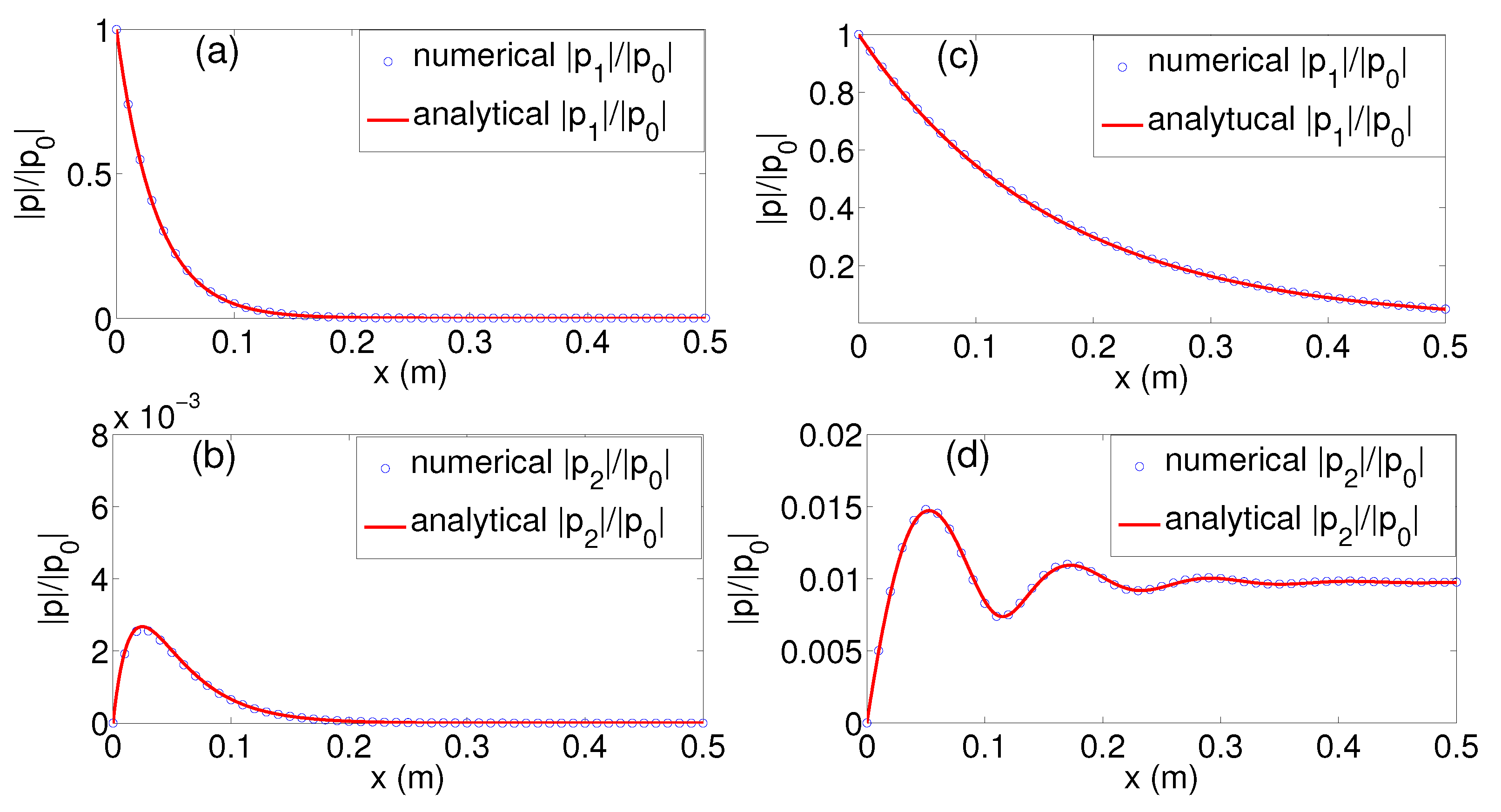
turns to 0, i.e., the generated second harmonic is due to the nonlinear effect. We can also find the second harmonic beatings in space, sin Δ k 2 χ in Equation (34). The position of the maximum of the beating can be related to the second-harmonic phase-mismatching frequency as
x c ( n ) = π Δ k n = π k ( n ω ) n k ( ω ) .
Therefore, as Δ k increases, the second harmonic beating spatial period, and also its maximum amplitude, decreases.

6. Results

Now, we study numerically the role of dispersion on harmonic generation, in the 1D acoustic metamaterial composed of elastic plates, and compare the numerical results to the analytical findings of Section 5. There are two cases, corresponding to the propagating driver and evanescent driver, which will be investigated separately below.

6.1. Driving Frequency in the Pass Band

We start by studying the case where both the fundamental component and the second harmonic component are in the pass band. We numerically integrate the weakly nonlinear lattice model, Equation (14), using an initial condition p 1 ( x = 0 ) of a cosinusoidal form, and also determine the spectrum of the solution by using the Fast Fourier Transform (FFT). Blue circles and red squares in Figure 4 show the evolution of the amplitude of the fundamental and second-harmonic components, respectively, as the wave propagates in the dispersive structure, as obtained numerically. As shown in the last section, if the distance between two cells is very small (here, we choose d = 0 . 01 m), the asymptote, a , in such a dispersive system will be very small—cf. green dotted line in Figure 2c—thus, the shock distance has a very small value. This means that the higher-harmonic generation process is achieved much closer to the source, compared to the Fubini solution (see Figure 3). The second-harmonic component p 2 / | p 0 | no longer increases linearly because of the presence of dispersion induced by the elastic plates. Notice that p 2 / | p 0 | develops beatings in space due to the phase mismatch. The fundamental wave vector of our source k 1 (frequency ω) generates a forced wave 2 k 1 (frequency 2 ω ), while the free wave that our system allows to propagate is k 2 . The difference between 2 k 1 and k 2 (because of the dispersion relation) introduces a phase mismatch, which means that the second harmonic generation is asynchronous. We can, therefore, clearly observe the beatings in Figure 4, where the analytical solutions have an excellent agreement with the numerical ones. This perfect agreement breaks down if we consider a driving frequency with a second harmonic higher than 1 kHz, since the continuous dispersion relation, see Equation (20), deviates from the discrete one. Additionally, since we have considered a weakly nonlinear regime, the agreement between numerics and our approximation is found to break down for amplitudes larger than 10 kPa. When we increase the frequency from 350 Hz to 400 Hz, Δ k decreases, x c increases, the second-harmonic beatings spatial period—and also its maximum amplitude—increase, see Equation (34). During the nonlinear propagation in the dispersive system, cumulative nonlinear effects generate harmonics of the fundamental frequency, and we can control this process by tuning the dispersion relation with either the properties of the array or that of the plates.

6.2. Driving Frequency in the Bandgap

When the driving frequency is in the band gap, its second harmonic may be located either in the gap band (evanescent) or in the pass band (propagating). In the former case, the second harmonic is damped, and its decay rate is given by the imaginary part of the dispersion relation. In the latter case, the second harmonic is propagating through the structure. Both cases are analyzed below.
We start by studying the case where both the fundamental component and its second harmonic are in the band gap. In this case, the dispersion relation does not support real solutions, so the corresponding wave number is imaginary, namely k ( ω ) = i k 1 , with k 1 the imaginary part of the wavenumber, given by the dispersion relation. When k 1 is very large, for example at f = 90 Hz, cf. Figure 5a, the fundamental component p 1 decreases exponentially very quickly, namely p 1 exp [ Im ( k ) x ] . The second harmonic component is generated at the beginning of the structure but is very small. In this case, k ( 2 ω ) = i k 2 , with k 2 the imaginary part of the wavenumber given by the dispersion relation for 2 ω . The generated frequency 2 f = 180 Hz is still in the band gap, the corresponding Im ( k ) is smaller than that of the fundamental frequency, but still very large. Therefore, we can find a very small p 2 / | p 0 | at the beginning of the structure, which eventually decreases to zero, see Figure 5b.
If the driving frequency is close to the first cut-off frequency, the frequency of the generated second-harmonic will be in the pass band. In this case, p 1 / | p 0 | decays slowly during the propagation because the imaginary part of k is very small, cf. Figure 5c, where f = 300 Hz, while the generated second-harmonic component is propagating, cf. Figure 5d. We can also find the second-harmonic beatings at the beginning due to the phase mismatch (the difference between 2 k 1 and k 2 ). Comparing to the result shown in Figure 4, the beating spatial period is smaller because of a bigger Δ k . The fundamental component is evanescent and, therefore, there will not be phase mismatch for p 2 (only k 2 propagates), i.e., we can hardly observe the beatings for p 2 / | p 0 | after 0 . 4 m, as shown in Figure 5d.

7. Conclusions

In conclusion, we have theoretically and numerically studied the nonlinear propagation and second-harmonic generation in 1D acoustic metamaterial composed of an air-filled tube with a periodic array of elastic plates. Based on the electro-acoustic analogy, we proposed the transmission line approach to derive a nonlinear lattice model, which was analyzed by both numerical and analytical techniques. Considering the continuum limit of the lattice model, we derived a nonlinear dispersive wave equation, in the form of a nonlinear Klein–Gordon model, which reduces—at certain limits—to other well-known acoustic wave models (such as the Westervelt equation). In the linear limit, we derived from this model the dispersion relation which, in the low frequency regime, was found to be in excellent agreement with the one obtained by the transfer matrix method. We have shown that, during the nonlinear propagation, cumulative nonlinear effects generate harmonics of the fundamental frequency. Dispersion introduces phase mismatch between at higher harmonics, which is the responsible of the beating effect. We used a perturbative approach to study analytically the effect of dispersion on the harmonic generation. Analytical and numerical results were found to be in excellent agreement.
There are many future research directions that may follow these preliminary results. First, it would be interesting to investigate if the combined effects of nonlinearity and dispersion may give rise to the emergence of solitons in the system (i.e., nonlinear waves that propagate undistorted when nonlinearity and dispersion are exactly counterbalanced). Second, taking into account the presence of inherent losses in the metamaterial structures under consideration, a study of the interplay between nonlinearity, dispersion and losses would be very relevant. It would also be interesting to extend our work to higher-dimensional settings, as well as to study nonlinear propagation in double negative metamaterials, waveguides periodically loaded with a combination of elastic plates and Helmholtz resonators.

Acknowledgments

This work has been funded by the Metaudible project, Agence Nationale de la Recherche, ANR-13-BS09-0003, co-funded by ANR and Fondation de Recherche pour l’Aéronautique et l’Espace (FRAE). Dimitris J. Frantzeskakis (D.J.F.) acknowledges warm hospitality at Laboratoire d’Acoustique de l’Université du Maine (LAUM), Le Mans, where most of his work was carried out.

Author Contributions

Vicente Romero-García (V.R.-G.), Georgios Theocharis (G.T.) and Olivier Richoux (O.R.) conceived the idea. Jiangyi Zhang (J.Z.) performed the analytics and the numerics. J.Z., V.R.-G., G.T., O.R., Vassos Achilleos (V.A.) and D.J.F. participate in the discussions and writing the article.

Conflicts of Interest

The authors declare no conflict of interest.

Appendix

Here, we analyze another variant of the unit-cell circuit, shown in Figure A1. Our purpose is to show that this variant leads to the same DDE model, Equation (14).
Figure A1. A variant of the unit-cell circuit for the nonlinear elastic plates lattice model: short segment of the waveguide before the elastic plate.
Crystals 06 00086 g006
First, Kirchoff’s voltage law leads to the equations
p n 1 p n = L ω d d t u n + L m d d t u n + 1 + V n ,
p n p n + 1 = L ω d d t u n + 1 + L m d d t u n + 2 + V n + 1 ,
which, when substracted, yield
δ ^ 2 p n = L ω d d t u n u n + 1 + L m d d t u n + 1 u n + 2 + V n V n + 1 .
Then, Kirchhoff’s current law yields
u n + 1 u n + 2 = C ω d d t p ,
where C ω depends now on p (and not on p n ) in this variant of the unit-cell circuit, where p is given by
p = p n + L ω d d t u n + 1 = p n 1 L m + 1 C m d 2 d t 2 d d t u n + 2 .
Additionally, current and voltage in the capacitor C m are connected by the equations
u n + 2 = C m d d t V n + 1 , u n + 1 = C m d d t V n .
Subtracting the two above equations, and using Equation (A4), we obtain
u n + 1 u n + 2 = C m d d t V n V n + 1 = C ω d d t p .
Thus, V n V n + 1 is expressed as follows:
V n V n + 1 = C ω C m p .
To this end, substituting the above results into Equation (A3) yields
δ ^ 2 p n = L ω + L m d d t C ω d d t p n + C ω C m p n .
Rearranging the terms, and recalling that the capacitance C ω depends on the pressure, we obtain the following DDE:
δ ^ 2 p n L C ω 0 d 2 p n d t 2 C ω 0 C m p n + L C ω 2 d 2 p n 2 d t 2 + C ω C m p n 2 = 0 ,
which is identical to Equation (14).

References

  1. Deymier, P.A. Acoustic Metamaterials and Phononic Crystals; Springer Series: Berlin/Heidelberg, Germany, 2013. [Google Scholar]
  2. Sugimoto, N.; Horioka, T. Dispersion characteristics of sound waves in a tunnel with an array of Helmholtz resonators. J. Acoust. Soc. Am. 1995, 97, 1446. [Google Scholar] [CrossRef]
  3. Bradly, C.E. Time harmonic acoustic Bloch wave propagation in periodic waveguides. Part I. Theory. J. Acoust. Soc. Am. 1994, 96, 1844. [Google Scholar] [CrossRef]
  4. Liu, Z.; Zhang, X.; Mao, Y.; Zhu, Y.Y.; Yang, Z.; Chan, C.T.; Sheng, P. Locally resonant sonic materials. Science 2000, 289, 1734. [Google Scholar] [CrossRef] [PubMed]
  5. Sánchez-Morcillo, V.J.; Pérez-Arjona, I.; Romero-García, V.; Tournat, V.; Gusev, V.E. Second-harmonic generation for dispersive elastic waves in a discrete granular chain. Phys. Rev. E 2013, 88, 043203. [Google Scholar] [CrossRef] [PubMed]
  6. Jiménez, N.; Mehrem, A.; Picó, R.; García-Raffi, L.M.; Sánchez-Morcillo, V.J. Nonlinear propagation and control of acoustic waves in phononic superlattices. C. R. Phys. 2016, 17, 543–554. [Google Scholar] [CrossRef]
  7. Remoissenet, M. Waves Called Solitons; Springer: Berlin, Germany, 1999. [Google Scholar]
  8. Sugimoto, N.; Masuda, M.; Ohno, J.; Motoi, D. Experimental demonstration of generation and propagation of acoustic solitary waves in an air-filled tube. Phys. Rev. Lett. 1999, 83, 4053. [Google Scholar] [CrossRef]
  9. Achilleos, V.; Richoux, O.; Theocharis, G.; Frantzeskakis, D.J. Acoustic solitons in waveguides with Helmholtz resonators: Transmission line approach. Phys. Rev. E 2015, 91, 023204. [Google Scholar] [CrossRef] [PubMed]
  10. Mingaleev, S.F.; Miroshnichenko, A.E.; Kivshar, Y.S.; Busch, K. All-optical switching, bistability, and slow-light transmission in photonic crystal waveguide-resonator structures. Phys. Rev. E 2006, 74, 046603. [Google Scholar]
  11. Kozyrev, A.B.; van der Weide, D.W. Nonlinear left-handed transmission line metamaterials. J. Phys. D 2008, 41, 173001. [Google Scholar] [CrossRef]
  12. Ogasawara, J.; Narahara, K. Experimental Characterization of Left-Handed Transmission Lines with Regularly Spaced Schottky Varactors. IEICE Electron. Express 2010, 7, 608. [Google Scholar] [CrossRef]
  13. Veldes, G.P.; Cuevas, J.; Kevrekidis, P.G.; Frantzeskakis, D.J. Quasidiscrete microwave solitons in a split-ring-resonator-based left-handed coplanar waveguide. Phys. Rev. E 2011, 83, 046608. [Google Scholar] [CrossRef] [PubMed]
  14. Veldes, G.P.; Cuevas, J.; Kevrekidis, P.G.; Frantzeskakis, D.J. Coupled backward- and forward-propagating solitons in a composite right- and left-handed transmission line. Phys. Rev. E 2013, 88, 013203. [Google Scholar] [CrossRef] [PubMed]
  15. Park, C.M.; Park, J.J.; Lee, S.H.; Seo, Y.M.; Kim, C.K.; Lee, S.H. Amplification of acoustic evanescent waves using metamaterial slabs. Phys. Rev. Lett. 2011, 107, 194301. [Google Scholar] [CrossRef] [PubMed]
  16. Lee, K.J.B.; Jung, M.K.; Lee, S.H. Highly tunable acoustic metamaterials based on a resonant tubular array. Phys. Rev. B 2012, 86, 184302. [Google Scholar] [CrossRef]
  17. Fleury, R.; Alú, A. Extraordinary sound transmission through density-near-zero ultranarrow channels. Phys. Rev. Lett. 2013, 111, 055501. [Google Scholar] [CrossRef] [PubMed]
  18. Bongard, F.; Lissek, H.; Mosig, J.R. Acoustic transmission line metamaterial with negative/zero/positive refractive index. Phys. Rev. B 2010, 82, 094306. [Google Scholar] [CrossRef]
  19. Rossing, T.D.; Fletcher, N.H. Principles of Vibration and Sound; Springer-Verlag: New York, NY, USA, 1995. [Google Scholar]
  20. Chandrasekharappa, G.; Srirangarajan, H.R. Nonlinear response of elastic plates to pulse excitations. Comput. Struct. 1987, 27, 373–378. [Google Scholar] [CrossRef]
  21. Hamilton, M.F.; Blackstock, D.T. Nonlinear Acoustics; Academic Press, AIP: San Diego, CA, USA, 1998. [Google Scholar]
Figure 1. (a) waveguide loaded with an array of elastic plates; (b) a corresponding unit-cell circuit of the nonlinear model of elastic plates lattice.
Crystals 06 00086 g001
Figure 2. (a) the dispersion relation of system analyzed in this work for the real wavenumber, in the regime of low frequencies. The blue dashed line shows the results from the transmission line approach (keeping up to the O ( d 4 ) ), the red line represents the ones obtained using the transfer matrix method and the black dash-dotted line stands for the dispersion relation obtained by using the transmission line approach keeping only up to O ( d 2 ) . The points in Figure 2a show the frequencies used later in the simulations, 350 Hz and 400 Hz; (b) the dispersion relation of our system in the regime of low frequencies for the imaginary part of wavenumber k. The blue dashed line shows the results from the transmission line approach (keeping up to the O ( d 4 ) ), the red line represents the ones obtained using the transfer matrix method and the black dash-dotted line stands for the dispersion relation obtained by using the transmission line approach keeping only up to O ( d 2 ) . The points in Figure 2b show the frequencies used later in the simulations, 300 Hz and 90 Hz; (c) the influence of the periodicity d of the lattice on the first cut-off frequency m (m is not the resonance frequency of the elastic plates f m , but in our system it is close to it) (blue line) and the influence of d on the asymptote of the quasi linear part a (green dashed line); and (d) the influence of the thickness of the elastic plates h on the first cut-off frequency m (blue line) and the influence of h on the asymptote of the quasi linear part a (green dashed line).
Crystals 06 00086 g002
Figure 3. Fubini solution, for the wave propagation in the waveguide without elastic plates, with f = 400 Hz. Solid and dashed lines depict analytical results, while circles and squares depict numerical ones. The black solid line and blue circles represent the fundamental component, while the dashed green line and red squares correspond to the second harmonic component. The numerical results have an excellent agreement with the Fubini solution.
Crystals 06 00086 g003
Figure 4. Harmonic generation in the presence of dispersion in the case of a propagating driver. Second harmonic develops beatings in space due to the phase mismatch. Circles and squares depict numerical results, while solid and dashed lines correspond to the analytical (perturbative) findings. Both p 1 / p 0 (upper) and p 2 / p 0 (lower) are in the pass band. (a) f = 350 Hz; (b) f = 400 Hz. Numerical and analytical solutions are in excellent agreement.
Crystals 06 00086 g004
Figure 5. Harmonic generation in the presence of dispersion in the case of a evanescent driver. Blue circles and red lines depict, respectively numerical and analytical results. (a) f = 90 Hz, p 1 / | p 0 | in the band gap; (b) f = 90 Hz, p 2 / | p 0 | in the band gap; (c) f = 300 Hz, p 1 / | p 0 | in the band gap; (d) f = 300 Hz, p 2 / | p 0 | in the pass band. Numerical and analytical solutions are in excellent agreement.
Crystals 06 00086 g005

