Security from the Adversary’s Inertia–Controlling Convergence Speed When Playing Mixed Strategy Equilibria


1
System Security Group, Institute of Applied Informatics, Alpen-Adria-Universität Klagenfurt, Universitätsstrasse 65-67, 9020 Klagenfurt, Austria
2
Center for Digital Safety & Security, Austrian Institute of Technology, Giefinggasse 4, 1210 Vienna, Austria
*
Authors to whom correspondence should be addressed.
Games 2018, 9(3), 59; https://doi.org/10.3390/g9030059
Submission received: 2 July 2018
/
Revised: 27 July 2018
/
Accepted: 7 August 2018
/
Published: 21 August 2018
(This article belongs to the Special Issue Game Models for Cyber-Physical Infrastructures)
Abstract
:Game-theoretic models are a convenient tool to systematically analyze competitive situations. This makes them particularly handy in the field of security where a company or a critical infrastructure wants to defend against an attacker. When the optimal solution of the security game involves several pure strategies (i.e., the equilibrium is mixed), this may induce additional costs. Minimizing these costs can be done simultaneously with the original goal of minimizing the damage due to the attack. Existing models assume that the attacker instantly knows the action chosen by the defender (i.e., the pure strategy he is playing in the i-th round) but in real situations this may take some time. Such adversarial inertia can be exploited to gain security and save cost. To this end, we introduce the concept of information delay, which is defined as the time it takes an attacker to mount an attack. In this period it is assumed that the adversary has no information about the present state of the system, but only knows the last state before commencing the attack. Based on a Markov chain model we construct strategy policies that are cheaper in terms of maintenance (switching costs) when compared to classical approaches. The proposed approach yields slightly larger security risk but overall ensures a better performance. Furthermore, by reinvesting the saved costs in additional security measures it is possible to obtain even more security at the same overall cost.
1. Introduction and Motivation
1.1. Playing a Mixed Strategy Causes Costs
Implementing a pure strategy equilibrium of a game is straightforward and the installation cost of the strategy occur only once at the beginning of the game since the optimal strategy profile is pure and will never be altered. When playing repeated games, however, it may occur that the optimal strategy is mixed, i.e., the optimal strategy is obtained by assigning a positive probability to two or more pure strategies. A mixed strategy is an assignment of probabilities, which declares a law for randomly selecting the individual pure strategies in each round of game to ensure an optimal result regarding the expected utility. In standard models it is assumed that players can switch strategies as frequently as they want. Yet, in real life switching strategies will incur additional costs. For example if we consider game-theoretic models in cybersecurity, strategies may include different configurations of servers, firewalls or other system components. If switching strategies means changing configurations, the change may be costly in terms of time or money (e.g., downtime of servers, hourly rates of staff, etc.).
One possibility to consider switching costs is to compute multiple Nash equilibria and choose the one with the smallest (Shannon) entropy. This approach yields the “purest” of all equilibria. Another possibility is to model the problem in terms of dynamic games: the aim is to find the optimal Markov chain, i.e., to find the best (mixed) strategy based on the current state and the cost of switching to new states. Rass, König and Schauer have discussed these approaches in [1]. They point out that solely considering “more pure” strategies (an thus reducing the frequency of action changes) or minimizing the costs for the next choice is not sufficient: the implementation of a defense strategy needs to be done in a way, such that the defender’s moves should not be predictable for an attacker, as this facilitates security breaches. In other words, when employing a security strategy it should not be possible to get a better forecast on the defender’s next action when considering the current state of the system and the costs incurred by switching to another strategy. Thus, instead of calling for a dynamic optimization [1], suggest a static framework, where all actions are taken stochastically independent of the current state while still minimizing the switching costs. Despite their strong focus on security principles, there exist even more efficient solutions if we take an “information delay” for the adversary into account, i.e., the time it takes the attacker to recognize a changed situation and adapt to it.
The concept introduced in this work incorporates the time it takes for an attacker to mount an attack. It may happen that an attacker does not have complete information about the present state of the attacked system (such as the current strategy of a defender), but only knows the state of the system some rounds ago. This may happen, for example, if it takes the attacker some time to carry out the attack, i.e., the adversary has some inertia. During this period, the attacker may not be able to keep track of the system, and will not detect if the state of the system changes. Thus, his attack is performed after some delay, during which no new information can be processed. As a vivid example, consider an intruder who tries to gain unauthorized access to some critical infrastructure, that is surrounded by a wall. Before he starts his attack, he knows the current position of a guard, as he can see him through a window or compromised camera, but while he is entering the premises, the position of the guard may change, without the attacker noticing.
In the following, we will refer to this scenario as an information delay. By taking into account the average time the system is unobservable for an attacker prior to his attack, we can construct strategy policies that are cheaper in terms of switching cost. This saving is traded for a slightly larger risk in the primary security goal, but ultimately yielding a better performance overall. Security is never only an economic matte of cost-benefit balance, and impractical security solutions are practically worthless (say, if the optimal security strategy prescribes frequent changes in server configurations, such a strategy would simply not be doable in practice). Taking into account the cost for “running” an optimal defense as such is, in our opinion, an equally important aspect of defense as the security precaution itself. This work aims at providing means to keep the running costs of a defense under control and in balance to the security benefits therefrom.
1.2. Related Work
This work essentially deals with convergence to a Nash equilibrium, which is a well studied matter in the literature, but usually with a totally different goal as ours. Some work [2] indeed assumes a certain “speed” of the attacker, and adapts the defense to it. However, this prior work (and related follow-ups) disregard the potential of moving slightly faster than the adversary to gain an explicit profit from this. Most studies of convergence relate to the speed at which behavior can be adapted to become optimal in the long run [3,4,5,6,7], with some consideration spent on specific settings such as congestion or load balancing. The cost borne in switching between configurations has been considered in [8], where the authors use entropy as a measure to prefer certain strategies with less cost in the change. In the context of password policy choice, [9] considered games about choosing passwords that are (i) easy to remember, (ii) hard to guess, and (iii) easy to change (for the owner). The latter aspect is a well known cause of passwords to follow certain patterns like having counters attached to them or similar. Taking the password change (switching) cost into account can aid looking for a best password policy and prevent the issue to some extent. Related on different grounds is also [10,11], where convergence to an (-approximate) equilibrium is studied using Markov chains. Our work relates to this in the sense that we also design Markov chains to play a desired equilibrium, but use an -approximation to the equilibrium as an area of trade-off to avoid costs from switching. In that sense, we provide a novel use of -approximations to equilibria for the sake of security economics [12].
1.3. Contribution and Structure of the Article
This contribution aims at generalizing the switching cost model [1] for games where the attacker has incomplete information that can be described by an information delay. By taking into account information delay, the implementation costs can be reduced while still ensuring the security principle that the opponent cannot forecast the next move more precisely. The resulting policy can be described using a Markov chain model. We will show in fact that the switching cost model is a special case of our information delay model.
The structure of the article is as follows: first, we introduce some preliminary concepts and notations required to describe the game setup as well as the costs for switching strategies in Section 2. In Section 3 and Section 4, the theoretical framework is explained and all mathematical derivations stated. A numerical example completes the Section 3. Finally, Section 5 summarizes the findings and highlights some open questions that might be relevant for future research.
2. Preliminaries
In the following, we will use uppercase letters to define random variables and sets. Vectors are printed in bold-face. We will write X∼F if a random variable X is distributed according to a probability distribution F. Distributions on finite ordered sets are described using probability vectors , which represent the probability mass function of the underlying random variable. It is assumed that the random variable follows a discrete distribution, hence it has a density w.r.t. the counting measure. We will use the notation to express that an element d was sampled from the set with distribution ; i.e., if d is the i-th element in the ordered set .
2.1. Definitions and Game Setup
We consider a finite two-player game between player 1 and player 2 with pure strategy sets and , respectively. Let and where . We write to denote the simplex over a strategy set that contains all probability distributions on . The extension to players will be obvious so we only consider the case with two players. We assume a zero-sum situation, i.e., the attacker (which is player two) has the payoff . In our security game scenario let us adopt the defenders perspective, i.e., we act as player 1 in the game. Throughout this work the defender’s strategies are determined by the expected damage and the switching costs. We assume that the defender is minimizing two objectives: the primary security goal is minimization of the damage due to a risk and the second goal is reduction of the switching cost.
2.2. Costs for Playing Mixed Strategies
The damage that is minimized as the first objective is modeled by a utility function : ,
that descries the expected damage depending on both players actions. For simplicity we assume is a constant matrix.
The second goal is switching cost minimization: by our definition, a switch from strategy to strategy will cause cost for player 1. Note that the cost of switching strategies only depends on player 1’s actions, i.e., on his past and present strategy which we denote by and respectively, and denotes the t-th gameplay. Thus, we can employ a first order Markov chain to describe the switching behavior. As the player’s switching costs, and therefore his next move, only depend on the present state the switching process is a first order Markov process. As any stochastic process is fully determined by its finite dimensional distribution, we can describe the switching behavior by specifying the joint probability distribution (jpd) of and , . As we assume the switching costs are constant over time, the optimal jpd that determines the mode of changing strategies will be constant over time as well. Thus, the resulting, optimal switching policy joint probability distribution of can be modeled as a time-homogeneous process, i.e., it holds . Homogeneity implies that expected switching cost can be described by
We now model the simultaneous optimization of damage and cost as a multi-objective game (MOG). In a MOG, each player i can have utility functions , defined over , where denotes the strategy space of the remaining players. In our two-player zero-sum game we have 2 objectives and both players have vector-valued payoffs , which yields the two-player zero sum MOG . For this situation the following definition is convenient.
Definition 1 (Pareto-Nash Equilibrium).
In game with a minimizing player 1, a Pareto-Nash equilibrium is a strategy profile that fulfills
where means that there exists at least one coordinate i for which holds, regardless of the other coordinates.
Lozovanu, Solomon and Zelikovsky [13] have studied the computation of Pareto-Nash equilibria by scalarizing the utility vector. To this end, each player i defines weights , to scalarize his utilities via . In [13] it was proven that the Nash equilibria of so scalarized games are exactly the Pareto-Nash equilibria in the original multi-objective game.
Letting the defender prioritize a set of two goals by assigning weights and , the scalarized payoff for the defender is
For readability we will drop the coefficients and as we can just include them in the constant matrices and .
2.3. The Switching Cost Model (SCM)
The model introduced in [1] assumes that the switching of strategies is performed independently of the current strategy, i.e., . Thus, any future change in strategy is not predictable with more accuracy when the current system state is known. Hence the utility function can be written as
This way, the whole behavior of the system can be described using only the marginal probability vectors :
with constant payoff matrices as well as . We stress the fact that need not be a symmetric matrix. As a simple example consider a security guard driving to different assets i and j where j is on top of a mountains and i in the valley. The ascend from i to j will certainly take up more resources (e.g., fuel) than the decent from j to i. Thus, holds indeed. Yet, we assume that (remaining in the current strategy does not incur any switching costs).
In absence of an accurate adversary model [14], we may strive for a worst-case analysis and assume that the attacker will always try to cause as much damage as possible, i.e., they aim to maximize over :
Note that for player 2 the expression is constant. Thus , where denotes the i-th coordinate unit vector. By substituting , the resulting problem can be described through the following optimization problem.
2.4. Extension of SCM–Taking into Account Information Delay
In this paper we extend the switching cost model by relaxing the independence assumption, i.e., we let the choice of the next pure strategy depend on the current state . Thus, we want to model the switching behavior as a Markov process. In order to reduce the switching costs, we may add some inertia to player 1 by increasing the conditional probability to remain in the current strategy for each state. Will control the amount of inertia in a way that we can guarantee the distribution of the system after a predetermined amount of gameplays k conditional on the last observed state to be almost the same as the unconditional distribution.
Hence, we demand the resulting marginal distribution after a fixed number k of consecutive repetitions of the game to be “almost independent” of the initial state, i.e., the conditional and unconditional probabilities after k or more steps need to be almost the same, that is we require
where is the sum of absolute deviations of the two probability vectors. We call k the information delay that specifies the length of the period an attacker is not able to gain insight into a system prior to attacking (see Figure 1). Furthermore we call the maximum deviation of independence. In a seemingly alternative view, one could propose wrapping up a lot of rounds of the game that are interdependent in a single “larger” round, yet such an approach could be flawed for two reasons: first, this would impose an independence assumption between any two batch of round in the game. Second, the timing of the game rounds may be naturally induced by the “periodicity” of the business as such (e.g., work hours per day, shifts, or similar).
In this dynamic framework we need to redefine the objective function . Obviously, there is a conflict in notation and conceptualization here when optimizing over plus , as is a function with arguments and , i.e., the arguments are the marginal distributions each players assign to his set of pure strategies, but (in contrast to the formulation in (3)) is a function of the joint probability distribution of player 1’s strategies. Yet, there is a direct connection between and : as we are dealing with mixed strategies, the defender will often switch pure strategies and by law of large numbers the distribution over pure strategies will converge to after an infinitude of gameplays. Accordingly, the dynamic (i.e., switching) behavior of player 1, which is described using a homogeneous discrete Markov chain (HDMC) needs to have as a stationary as well as the unique limiting distribution in order for the two objective goals to be consistent.
Bearing in mind that the limiting behavior of any HDMC can be described using a one-step transition matrix of dimension and an initial distribution that describes the starting state of the process, we will make use of the following theorems for our results:
Theorem 1.
(Limit [15]) Every aperiodic irreducible HDMC with finite state space has a unique limiting state π.
So if we are dealing with aperiodic irreducible homogeneous discrete Markov chains with finite state space we can ensure the existence of a unique limiting state , which is always a stationary state. Additionally, it can be shown that the limiting distribution of a such a stochastic process is independent of the initial distribution . Moreover, by the following ergodic theorem, it is possible to specify the speed of convergence to the limit state for an aperiodic irreducible HDMC with finite state space and transition matrix . Let denote the transition probability from state to after k steps. Note that the following theorem is a consequence of the Perron-Frobenius Theorem. 1
Theorem 2.
(Geometric Ergodicity [16]) Let the transition matrix of an irreducible, aperiodic Markov chain with finite state space . Then for all probability vectors if holds
, for all and π is the only solution to
Moreover, the speed of convergence to the limiting state π is geometric, i.e., there exists a constant (that depends on only) such that
is the row vector with all ones, denotes the second largest eigenvalue of in terms of absolute values.
The following proof is from [17]. We will limit ourself tho the case when is diagonalizable, which is the case for our construction of .
Proof.
An irreducible aperiodic Markov chain has a positive transition matrix . Let , , denote the right eigenvectors of and , , the left eigenvectors of .
By Perron-Frobenius Theorem the largest eigenvalue is unique and possesses a strictly positive left eigenvector. For stochastic matrices like it additionally holds that the largest eigenvalue is , the right eigenvector to is and its left eigenvector is the one that fulfills (5). Thus, .
Now we can write in its spectral representation where . As if and if , we have
As we have
Now for all initial states i and resulting states j the absolute difference of the components of and the corresponding entries in (i.e., ) is bounded by
where denotes the respective entry of , .
Finally yields
Finally, taking
we get the Expression (6). ☐
Geometric ergodicity means that the absolute difference of the steady state to the marginal distribution after k steps given any initial distribution is bounded by . Subsequently, determines the speed of convergence to the steady state distribution given an arbitrary initial distribution : The smaller , the faster the convergence to the steady state. Considering Equation (4) it is obvious, that if we want the distributions of and for an arbitrary instantiation of to differ by at maximum , we need to control the second largest eigenvalue of , i.e.,
.
Now we want construct an irreducible aperiodic HDMC described by a transition probability matrix of a for which it holds
- -Convergence: the resulting conditional probabilities after k or more repetitions of the game given an initial are approximately the ergodic state (i.e., they satisfy (4))
- Equilibrium: the limiting as well as the marginal distribution of the process equal the Nash-Equilibrium-solution from (3)
- Cost reduction: the total costs are reduced.
In (8) have seen that -convergence can be achieved by controlling the second largest eigenvalue of the conditional probability matrix. The following result will help construct the sought transition matrix for the intended convergence control:
Theorem 3.
(Sklar [18]) Every cumulative distribution function of a random vector can be expressed by its marginal distributions and a copula such that .
Note that we are dealing with first order HDMCs and that the whole behaviour of the chain is determined by one single two-dimensional joint distribution function for all , i.e., . For brevity, we will abbreviate by . As we require both the marginal probabilities of and to equal the Nash-Equilibrium-solution from (3), the joint distribution of the random vector can be constructed using the marginal distribution of only, i.e., .
Using Sklar’s Theorem and the fact that we are only considering absolutely continuous discrete random variables with -finite measures , the first order Markov Process has not only a joint cdf, but also a discrete density . Thus, there exists an , for which it holds that for all : , for all j and for all i. Therefore, the discrete density, which is represented by , has marginals prescribed by and we hereafter write to denote this dependency. As such , is not necessarily a function of , but rather chosen in a way constrained by regarding the marginals.
Under the above-mentioned prerequisites, we are able to redefine so that it only depends on :
for the just defined joint probability matrix , .
Note that it is necessary to specify parametric functions to model the jpd, as parameters are not estimable given the number of constraints. It is not possible to directly optimize the individual over . Therefore, we need to constrain f to a parametric family of functions, i.e., , where the optimization is performed by adjusting the parameter vector . Then, given which represents, the respective one step transition matrix can directly be computed via
where is a diagonal matrix. Unfortunately, even when using parametric families of functions for f in most cases controlling the value of from will be difficult. For reversible Markov chains one could compute upper bounds via Cheeger’s and Poincare’s inequality [19], yet we will work with a direct construction scheme for for which it is possible to obtain exact control of .
3. Efficient Switching by Considering Information Delay
In the defined framework it is possible to construct an aperiodic irreducible HDMC with state space that satisfies -convergence as well as the equilibrium condition while reducing costs at the same time.
To do so, we first set the parameters
- : the information delay
- : the maximum deviation from the steady state distribution after k rounds of game play when an arbitrary initial state is given.
W.l.o.g. we assume is the last instantiation of the process which is known to the attacker. In the next step we compute the optimal solution for from (3). Then, using we will only include those pure strategies in our framework for which holds in Theorem (3). Excluding zero probability states is necessary, as otherwise the transition Matrix that we will construct is not positive, which is a necessary condition in Theorem 2. W.l.o.g. denote the included strategies , and their probability vector . For the class of functions f we choose the following family that depends on one parameter and the probability vector :
W.l.o.g. let the 0 entries of be . For f we can easily prove the following:
- for all with ,
- for all with ,
Now observe that by the definition of f in (10) statement (9) is equivalent to
which yields
where denotes the identity matrix and is the vector of all 1s. Note that by strict positivity of the constructed HDMC with one step transition matrix is aperiodic and irreducible. Furthermore, the so constructed Markov chain has the limiting state , i.e., the limiting marginal distribution of the chain is the Nash-equilibrium solution from (3).
In this setting it can easily be verified that the largest eigenvalue of is 1 and that all remaining eigenvalues are :
Theorem 4.
The second largest eigenvalue of is and has algebraic multiplicity .
Proof.
The characteristic polynomial of is
Thus, in order to determine the eigenvalues of we need to determine the eigenvalues of and it holds2:
As consists of equal rows the rank of is one. Thus, there exists only one eigenvalue of which is not 0. As the trace of is the sum of its eigenvalues, and , it holds
Thus, and . ☐
Thus, we have proven that by proper choice of f and we can control the switching of policies in the way we need it. Furthermore, as we remain in the current position more often, the costs of switching are reduced while it is ensured that the marginal distribution converges after a predetermined number of rounds k at a given accuracy .
By construction of and the fact that for all it furthermore holds
Thus, we can reduce the initial switching costs by a proportion of .
This way using a homogeneous discrete Markov chain we can describe a policy that employs lower average switching cost, while still controlling the damage caused by adversaries. Of course (11) is not the only construction scheme for that allows for a direct control of . There certainly exist other ones employing different copulae with similar characteristics. We chose the upper construction due to its simplicity and elegant properties regarding its second largest eigenvalue.
We will now prove a sufficient condition, when the general cost can be reduced while obtaining almost the same security. In the following it is again assumed that the scalarization constants are already included in the payoff matrices. Furthermore, assume that the information delay k is given. As mentioned before, in the information delay model we only include those strategies , where , that is we consider , , .
Let denote the conditional probability vector after steps, i.e., is the colum of the positive transition matrix:
Now assume it takes an attacker steps to carry out an attack. Then, by the law of total probability and (12), the total utility for player one when considering information delay is given by
where denotes the payoff matrix where all rows of states with were deleted, and is defined analogously. Setting , , yields (2).
Now by loosening the independence assumption to lower the switching costs, we deviate from the optimal (under independent sampling of strategies) solution , which might increase the value of the first objective function . The total cost incurred after steps is reduced if the reduction of switching costs is higher than the increase in the value of the first objective function , i.e., if
which yields
or by deletion of the zero-entries in and the correspronding rows in :
Expression (16) states that the total cost can be guaranteed to be reduced if the switching cost reduction is larger than the costs incurred by deviating from . We will now show, how can be chosen with respect to a given maximum deviation of independence in order to ensure a total cost reduction. First, assume that (4) holds; a sufficient criterion for this to hold is . By (7) . Then, for the resulting conditional probability vector with information delay, it holds for all and for all :
and as the maximum deviation from independence is we have
Thus, we have proven the following theorem:
Theorem 5 (Cost reduction).
This implies that, if and satisfy the condition (18), then the total costs are reduced. The following example illustrates the results.
3.1. Example and Sensitivity Analysis
Consider the following two-player zero-sum Matrix-game with switching costs. We define the parameters
For simplicity it is assumed that the scalarization constants are already included in the payoff matrices. Furthermore, assume that the information delay is .
The standard equilibrium (we will denote it as ), if we only consider , is with a value . The cost of switching strategies independently, as it is assumed in standard models, however, would incur an extra cost of per round, which yields in total.
Now, computing from (3) yields . The switching costs are and the maximum damage caused by the adversary is . This yields average costs of in each repetition of the game. Note that this strategy only includes the first and the last strategy .
We will lower this average cost by taking into account the adversaries inertia, which is represented by the information delay of rounds. As mentioned before, in the information delay model we only include those strategies j, where , hereafter denoted as , and . By (7), . In our case the matrix has left eigenvectors and right eigenvectors . Thus,
Solving the inequalities and from (18) for yields . Replacing the inequalities by equalities we obtain and , i.e., if the adversary knows the initial state, the individual conditional probabilities after 3 or more steps will differ from each component by about a quarter of a percent point at maximum.
Inserting into for it can be seen that the maximum deviation to the components of is indeed no more than :
For the switching costs are and the value for is obtained using Expression (13):
Thus, the total average cost incurred is . The switching costs were reduced by in each round, while the maximum damage caused by an adversary was only increased by . Henceforth, taking into account the adversaries inertia can cause a dramatic cost reduction, while still ensuring almost the same security.
Remark 1.
Another possibility to find admissible θ is to apply the bisection method to θ until the maximum deviation of the entries of to is smaller than a predetermined ϵ. As an example we chose and obtained , which yields even lower switching costs (). We obtained
In this case, the average value of is and the total cost per round is .
4. Minimizing the Total Cost
If one wishes not only to find a way to efficiently implement the Nash-equilibrium solution from (3), but also allows for other ergodic states to minimize the total cost while still ensuring -convergence after k steps, one can rewrite the utility function (13) using the transition matrix :
Here, k is is the information delay (an input parameter), and is an probability vector over , that only includes non-0-probability strategies from . , likewise denote the cleaned from zeros payoff and switching cost matrices only including the strategies from E. For , the transition matrix is defined as . The global optimum can then be found by solving the following optimization problem:
subject to , , , . The optimization is performed in the following way: first, it is decided which stategies from to include in E. i.e., we choose a subset of stategies from and w.l.o.g denote them . Then, the matrix is reduced to , which obtained by deleting all rows of stategies that are not included in E. Analogously, is obtained by deleting all columns and rows of strategies . Having obtained and and using the spectral representation of we can reformulate (20):
subject to , , , . Note that all , depend continuously on .
5. Discussion
It is interesting to note that despite optimality-by-design, some short-term deviations from an equilibrium can indeed be rewarding. Extending the concepts put forth in this work to dynamic games (e.g., leader-follower scenarios) is a natural next step. The methods used here lend themselves also to a treatment of perhaps continuous time chains, as limits of sequences of discrete chains with vanishing pauses in the limit. For practical matters, our work can provide a tool to fix implausible or impractical equilibria, by avoiding “hectic” changes if the equilibrium is mixed, while retaining a good security-investment trade-off. In the end, reinvesting the saved cost in additional security measures will yield even more security at the same cost.
At first glance our result seem to contrast earlier findings. For example, Reference [20] states that a defending player may actually benefit from revealing information about the defense strategy to the adversary and Reference [21] suggest that centrally allocating resources and publicly announcing the defensive allocation yields higher success probabilities for a defender. Both approaches deal with publicly announcing defense strategies to influence alleged attackers. This is different from our situation as we do not consider influencing the attacker (neither by providing potentially misleading information nor by hiding information). Rather we investigate how players behave if an information delay is part of the setting of the game, i.e., if it needs to be taken into account due to the situation at hand.
Author Contributions
Conceptualization, J.W.; Formal analysis, J.W.; Funding acquisition, S.R.; Investigation, J.W.; Methodology, J.W.; Project administration, S.R.; Resources, J.W.; Supervision, S.R.; Validation, J.W., S.R. and S.K.; Visualization, J.W.; Writing—original draft, J.W., S.R. and S.K.; Writing—review & editing, S.R. and S.K.
Funding
This research was funded by the project Cross Sectoral Risk Management for Object Protection of 290 Critical Infrastructures (CERBERUS) by the Austrian Research Promotion Agency under grant no. 854766.
Conflicts of Interest
The authors declare no conflict of interest.
Abbreviations
The following abbreviations are used in this manuscript:
| SCM | Switching Cost Model |
| jpd | Joint Probability Distribution |
| HDMC | homogeneous discrete Markov chain |
References
- Rass, S.; König, S.; Schauer, S. On the Cost of Game Playing: How to Control the Expenses in Mixed Strategies. In Decision and Game Theory for Security; Rass, S., An, B., Kiekintveld, C., Fang, F., Schauer, S., Eds.; Springer: New York, NY, USA, 2017; pp. 494–505. ISBN 978-3319687100. [Google Scholar]
- Dijk, M.; Juels, A.; Oprea, A.; Rivest, R.L. FlipIt: The Game of “Stealthy Takeover”. J. Cryptol. 2013, 26, 655–713. [Google Scholar] [CrossRef]
- Fudenberg, D.; Levine, D.K. The Theory of Learning in Games; MIT Press: London, UK, 1998. [Google Scholar]
- Chien, S.; Sinclair, A. Convergence to approximate Nash equilibria in congestion games. Games Econ. Behav. 2011, 71, 315–327. [Google Scholar] [CrossRef] [Green Version]
- Even-Dar, E.; Kesselman, A.; Mansour, Y. Convergence time to Nash equilibrium in load balancing. ACM Trans. Algorithms 2007, 3, 32. [Google Scholar] [CrossRef] [Green Version]
- Even-Dar, E.; Kesselman, A.; Mansour, Y. Convergence Time to Nash Equilibria. Lect. Notes Comput.Sci. 2003, 2719, 502–513. [Google Scholar] [Green Version]
- Pal, S.; La, R.J. Simple learning in weakly acyclic games and convergence to Nash equilibria. In Proceedings of the 53rd Annual Allerton Conference on Communication, Control, and Computing, Monticello, IL, USA, 29 September–2 October 2015; IEEE: Piscataway, NJ, USA, 2015; pp. 459–466. [Google Scholar]
- Zhu, Q.; Başar, T. Game-Theoretic Approach to Feedback-Driven Multi-stage Moving Target Defense. In 4th International Conference on Decision and Game Theory for Security—Volume 8252; GameSec 2013; Springer-Verlag, Inc.: New York, NY, USA, 2013; pp. 246–263. [Google Scholar]
- Rass, S.; König, S. Password Security as a Game of Entropies. Entropy 2018, 20, 312. [Google Scholar] [CrossRef]
- McDonald, S.; Wagner, L. Using Simulated Annealing to Calculate the Trembles of Trembling Hand Perfection. In Proceedings of the 2003 Congress on Evolutionary Computation, Canberra, Australia, 8–12 December 2003. [Google Scholar]
- Hespanha, J.P.; Prandini, M. Nash equilibria in partial-information games on Markov chains. In Proceedings of the 40th IEEE Conference on Decision and Control, Orlando, FL, USA, 4–7 December 2001; IEEE: Piscataway, NJ, USA, 2001; pp. 2102–2107. [Google Scholar]
- Anderson, R. Why information security is hard—An economic perspective. In Proceedings of the 17th Annual Computer Security Applications Conference (ACSAC 2001), New Orleans, LA, USA, 10–14 December 2001; pp. 358–365. [Google Scholar]
- Lozovanu, D.; Solomon, D.; Zelikovsky, A. Multiobjective Games and Determining Pareto-Nash Equilibria. Bul. Acad. Stiint. Republicii Mold. Mat. 2005, 49, 115–122. [Google Scholar]
- Rios Insua, D.; Rios, J.; Banks, D. Adversarial Risk Analysis. J. Am. Stat. Assoc. 2009, 104, 841–854. [Google Scholar] [CrossRef]
- Parzen, E. Stochastic Processes; Dover Publications, Inc.: Mineola, NY, USA, 2015. [Google Scholar]
- Cinlar, E. Introduction to Stochastic Processes; Springer-Varlag: New York, NY, USA, 1975. [Google Scholar]
- Lorek, P. Speed of Convergence to Stationarity for Stochastically Monotone Markov Chains. Ph.D. Thesis, University of Wroclaw, Wroclaw, Poland, 2007. [Google Scholar]
- Sklar, A. Fonctions de répartition à n dimensions et leurs marges. Publ. Inst. Stat. Univ. Paris 1959, 8, 229–231. [Google Scholar]
- Diaconis, P.; Stroock, D. Geometric bounds for eigenvalues of Markov chains. Ann. Probab. 1991, 1, 36–61. [Google Scholar] [CrossRef]
- Cotton, C.; Li, C. Profiling, screening and criminal recruitment. J. Public Econ. Theory 2014, 17, 964–985. [Google Scholar] [CrossRef]
- Bier, V.; Oliveros, S.; Samuelson, L. Choosing what to protect: Strategic defensive allocation against an unknown attacker. J. Public Econ. Theory 2007, 9, 563–587. [Google Scholar] [CrossRef]
| 1. | Note that by Perron-Frobenius Theorem for aperiodic irreducible HDMCs with finite state space the largest eigenvalue of the transition matrix is always 1 and its eigenvector is the steady state distribution. Further, the second largest eigenvalue that determines the speed of convergence to the steady state. |
| 2. | Note that the eigenvectors of and are equal, as rescaling and adding a multiple of does not alter the eigenvalues. |
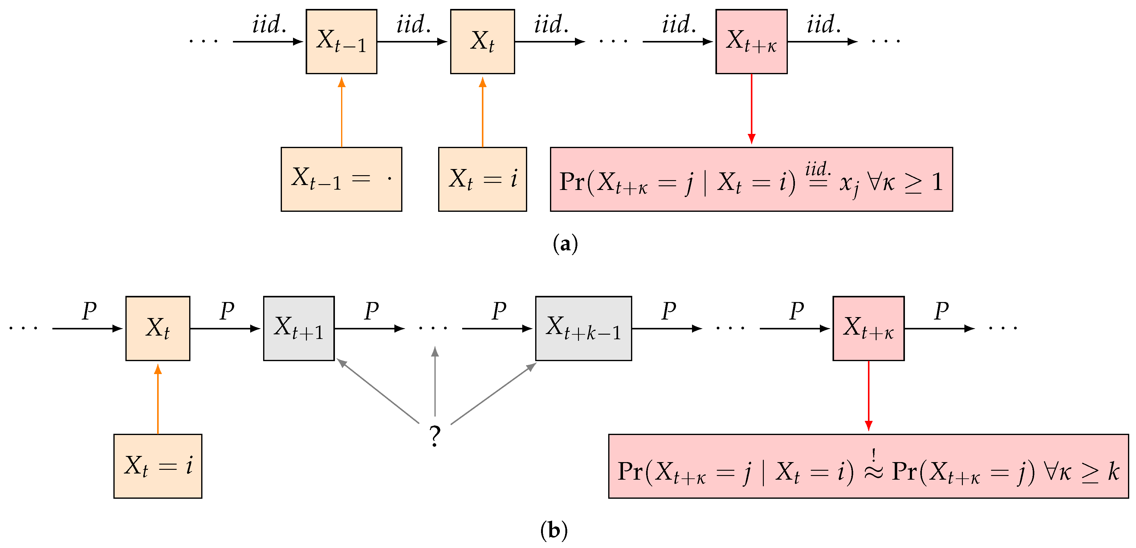
Figure 1.
Comparison of switching cost optimization in [1] to our approach. (a) Model in [1] assumes independent choice of next pure-strategy; (b) Our model allows for first-order dependence when choosing next pure-strategy but controls the deviation from the independence assumption after k or more subsequent gameplays.

© 2018 by the authors. Licensee MDPI, Basel, Switzerland. This article is an open access article distributed under the terms and conditions of the Creative Commons Attribution (CC BY) license (http://creativecommons.org/licenses/by/4.0/).
Share and Cite
MDPI and ACS Style
Wachter, J.; Rass, S.; König, S. Security from the Adversary’s Inertia–Controlling Convergence Speed When Playing Mixed Strategy Equilibria. Games 2018, 9, 59. https://doi.org/10.3390/g9030059
AMA Style
Wachter J, Rass S, König S. Security from the Adversary’s Inertia–Controlling Convergence Speed When Playing Mixed Strategy Equilibria. Games. 2018; 9(3):59. https://doi.org/10.3390/g9030059
Chicago/Turabian StyleWachter, Jasmin, Stefan Rass, and Sandra König. 2018. "Security from the Adversary’s Inertia–Controlling Convergence Speed When Playing Mixed Strategy Equilibria" Games 9, no. 3: 59. https://doi.org/10.3390/g9030059
Note that from the first issue of 2016, this journal uses article numbers instead of page numbers. See further details here.