Fairness-Adjusted Laffer Curve: Strategy versus Direct Method

Graduate School of Economics (GSE), Waseda University, Tokyo 169-8555, Japan
Games 2018, 9(3), 56; https://doi.org/10.3390/g9030056
Submission received: 21 June 2018
/
Revised: 25 July 2018
/
Accepted: 31 July 2018
/
Published: 2 August 2018
Abstract
:This paper reports results from controlled laboratory experiments on the Laffer curve and explores the productivity differences under the strategy method and the direct method. The data collected in Pakistan show no significant productivity difference across the two methods. The paper argues that the Laffer curve is not the result of a simple leisure—income tradeoff; the disutility of work and perceived unfairness of the tax imposed also influence the work decisions. A behavioral model that incorporates these factors induces a “fairness adjusted” Laffer curve with the negative relationship between tax rate and tax revenue showing up after 54% tax rate.
1. Introduction
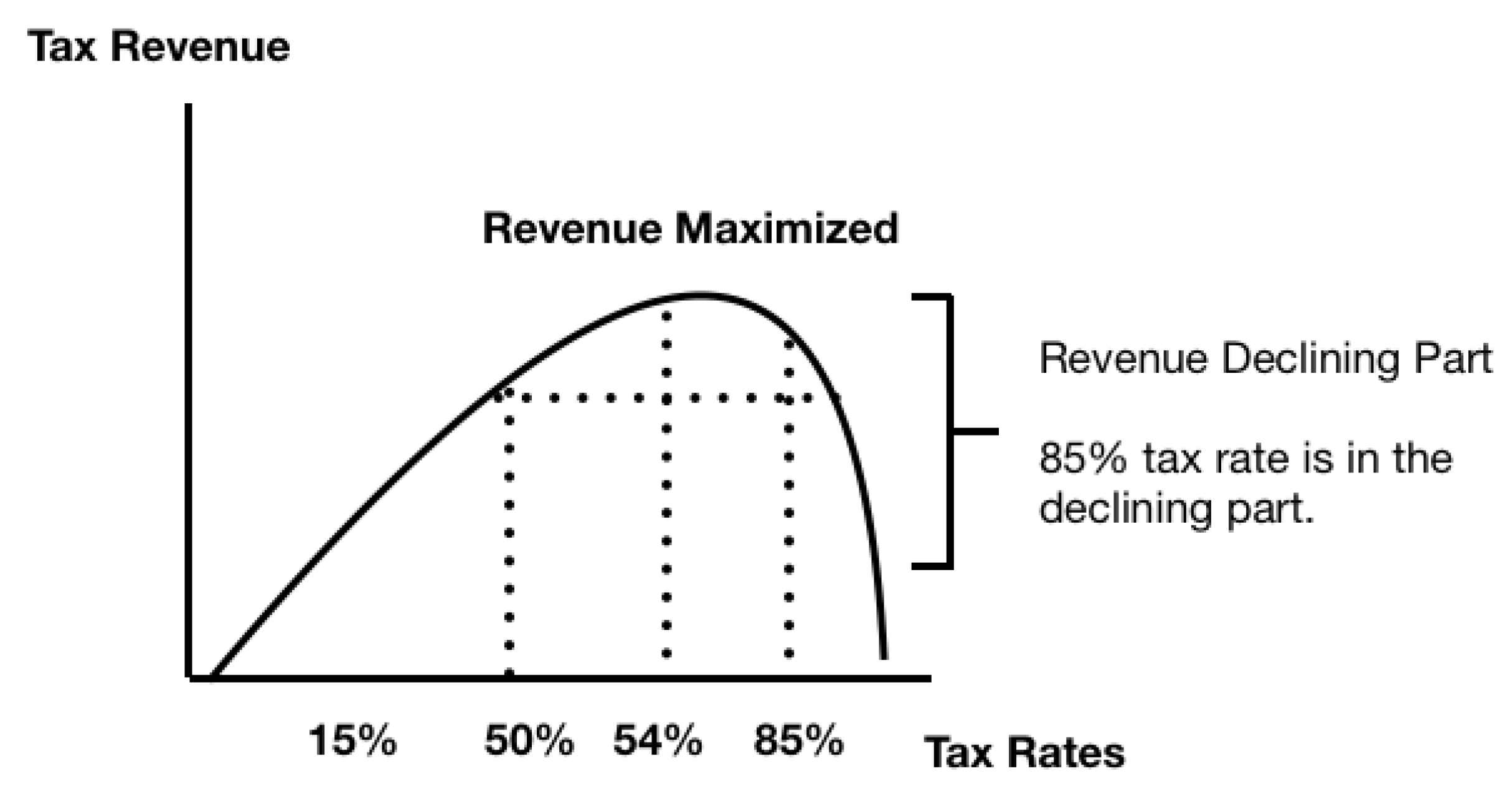
Income taxes are an important source of revenue for the government. Identifying optimal tax to extract maximum revenue has always been the goal of public policy makers, even in the ancient times. Ibn Khaldun [1] was the first one to identify the tax rates–tax revenues and tax rates–labor supply relationships, in the 14th century. He argued lower tax rates encourage labor activities, increase the tax base and tax revenues as well. Six centuries later, Laffer [2] formalized this relation between tax rates and tax revenues in the shape of the Laffer curve. The Laffer curve shows for a tax rate of zero percent there will be no tax revenue and for a tax rate of 100%, no one would work preferring to consume leisure and hence the revenue will be zero as well. In between the two extreme tax rates, there is a unique tax rate that maximizes the tax revenue. The Laffer curve has been studied in the experimental lab by various researchers. Thus far, there is one established result in the experimental literature pertinent to the Laffer curve: endogenous tax setting in the lab leads to the observance of the Laffer curve irrespective of the method by which the tax is implemented [3,4]. On the other hand, the results for the exogenous tax setting are dependent on the experimental method (direct versus strategy) and do not always lead to the observance of the Laffer curve in the lab. From a methodological viewpoint, the comparison among the methods (direct versus strategy) under the exogenous tax setting needs special attention as the results in the literature pertinent to these methods do not converge and previous Laffer curve studies do not offer a comparison among these methods.
The traditional Laffer curve approach relies on the income–leisure tradeoff to predict the labor supply and tax revenues while offering limited explanation on the relationship between the human behavior and taxation. To explain the social movements such as tax revolts and predict the effects of taxes on the labor supply with a greater accuracy, it is important to incorporate behavioral aspect of perceived unfairness of taxation in the Laffer curve theory. Moreover, the perceived unfairness of tax can also cause actions such as tax avoidance, tax evasion and hence cause a decline in the tax revenue of a government [5,6,7]. Along with direct impacts, the perceived unfairness of taxation can have spillover effects as well in the shape of low productivity, shirking and more frequent sick leaves [8]. On the other hand, a tax perceived as fair will encourage labor activities, promote a sense of satisfaction among the citizens and encourage tax compliance [9]. Hence, identifying optimal tax rates that maximize revenue and are perceived as fair is important for promoting the labor activities, tax compliance and maximizing the social welfare. Garboua at al. [4] were the first to make such an attempt by incorporating perceived unfairness in the theory of the Laffer curve. The focus of their work is on the outcome of an interaction between two players (a tax setter and a worker) with tax acting as endogenous variable in the interaction and the workers reduce their labor supply for tax rates exceeding 50%. Their work incorporates fairness in a specialized setting where it is difficult to conclude whether the reduction in the labor supply for tax rates exceeding 50% is due to the magnitude of the tax rate itself or due to the reciprocal behavior shown by workers towards the tax setters. Moreover, in real life, the governments decide tax rates exogenously and the magnitude of the reciprocal behavior is expected to be minimum under such a setting, while the positive or negative reaction to the magnitude of the tax rate is expected to derive the labor supply decisions. Hence, the fairness model proposed by Garboua at al. [4] does not seems to isolate the perceived unfairness of the tax magnitude from the reciprocal behavior that arises due to the endogenous tax setting. This paper makes important contribution to the existing literature by constructing a behavioral model that predicts the labor supply decisions based on the perceived unfairness of the magnitude of the tax and the disutility of the work while separating the impact of perceived unfairness of tax from the reciprocal behavior. The work of Garboua at al. [4] predicts the labor supply decisions only under the endogenous tax setting; the model proposed in this paper predicts the labor supply decisions and the Laffer curve under exogenous tax setting. Furthermore, as participants themselves declare the perceived unfairness about the tax rate, the model can intuitively explain the behavior under the endogenous tax rate as well. In addition to the proposed model, the paper contributes to the methodology of the Laffer curve experiments by reporting productivity comparison between the direct and the strategy methods, and is the first one to do so. The results from the experiments conducted in Pakistan show the average productivity of participants does not differ across the two methods. A model based on the disutility of work and perceived unfairness about the taxation indicates that a fairness adjusted Laffer curve exists with the tax revenue being maximized at 54% tax rate.
2. Related Literature
A typical lab experiment exploring the Laffer curve requires participants to solve real effort tasks for money. The experimenter observes the labor supplied under earning options that are varied by a change in the tax rates. The participants are often offered money as a substitute for the leisure to replicate the real life income–leisure trade off in the experimental lab. Our experimental design is identical to this typical one with certain important modifications explained below.
In this paper, the direct method refers to the actual choices made by participants in an experiment, while the strategy method refers to the provision of the complete set of strategies conditional on the experimental conditions [10]. In the direct method, participants actually solve the real tasks under various tax rates while in the strategy method participants disclose the number of tasks they would like to solve under various tax rates. The direct method offers an incentivized response to a tax rate after an effort has been exerted while the strategy method does it before an effort has been exerted. If the participants have a completely correct understanding about their abilities and effort costs in solving the experimental tasks, the two methods would lead to identical results. However, they can also lead to different results because the hypothetical nature of the strategy method tends to minimize the behavioral aspects during the decision making process. As a result, participants can behave differently when making an actual choice (as in the direct method) versus a probable choice contingent on various parameters (as in the strategy method). On the other hand, strategy method offers two important benefits: (1) As participants provide a complete set of choices contingent on all possible experimental conditions, they are expected to make an informed choice taking into account the consequences of all possible actions. (2) The provision of a complete strategy set provides better understanding of the decision-making process as well as potential motives of the participants. On top of these, it is also a cost-efficient method to collect the data [10].
In the current paper, participants were given three different earning options based on three tax rates in the direct method. Each of these earning conditions was 6 min long. In the strategy method under the same earning options, participants declared the number of tasks they would solve in 6 min. This time limit was enforced to make the results of both methods comparable. The enforcement of the time limit made participants consider their willingness to solve the tasks as well as belief about their efficiency in solving the tasks. This can have confounding effects on the dependent variable being measured. To minimize this confounding effect and to assist participants in forming correct beliefs about their efficiency in solving the tasks, a practice round of 6 min was introduced at the start of the strategy method. Participants solved the tasks in 6 min and were provided a feedback about the number of correctly solved tasks.
Keser et al. [11] studied the Laffer curve using the strategy method with exogenous tax in the experimental lab under three treatments. In the first treatment, tax revenue is redistributed among the participants; in the second treatment, the tax revenue is not distributed; and, in the third treatment, the tax revenue is used to provide a public good at a global scale. Tax rates are distributed from 0% to 100% with an increment of 5%. The results confirm that Laffer curve exists for all three treatments. Moreover, participants reduce their effort in all treatments as the tax rate increases. The reduction in the effort is highest for the treatment without the tax redistributions and is lowest for treatment with the tax redistributions. Garboua et al. [4] studied the Laffer curve using the strategy method under exogenous and endogenous taxation. They used 28%, 50% and 79% tax rates in the experiment. The endogenous tax treatment is conducted in groups having two participants. One of the participants in the group first selects the tax rate and later the other participant decides the effort level. No Laffer curve is reported for the exogenous treatment while for the endogenous treatment Laffer curve emerges at 50% tax rate. Sutter and Hannemann [3] used the strategy method with endogenous tax to study the existence of the Laffer curve. Each group consists of two participants where one assigns the tax rate and other one works. The Laffer curve emerges at 55% tax rate. Ottone and Ponzano [12] also used the strategy method with exogenous tax rates to study the Laffer curve. They used two treatments, with and without tax redistributions. The combined data for both treatments show a symmetric Laffer curve at 50% tax rate.
Swenson [13] used the direct method and exogenous tax to study the relation between tax rates and tax revenues and the impacts of tax rates on the labor supply decisions of the participants. The experiment uses unique task of typing exclamation mark on the keyboard. Another distinct feature of his work is the use of leisure options for participants who are not willing to work. Even though leisure options are limited to just 3, they represent the work–leisure tradeoff. Out of 18 participants, the Laffer curve and backward bending labor supply is observed for only eight participants. Fochmann et al. [14] studied the work duration and productivity under tax and no-tax treatments such that the net wage earned in both the treatments is identical. Subjects work more and have higher productivity in the tax treatment as compared to the no-tax treatment.
3. Experimental Design and Procedures
We explore the presence of Laffer curve using the direct and the strategy methods. In real life, the government exogenously sets taxes and hence we also use exogenous taxes. Addition of two digit numbers is used as the task in the experiment based on the work of Sutter and Hannemann [3]. Students are expected to solve these basic addition problems and they require considerable effort as well.
The experiments were performed in Pakistan. Gross wage of 3 Pakistani rupees per task was used in the experiment. Three tax rates of 15%, 50% and 85% were used and these tax rates give net earnings of 0.45 rupees, 1.5 rupees and 2.5 rupees per task, respectively. The tax rates were selected based on the work of Garboua et al. [4], who also used 3 tax rates (28%, 50% and 79%) in their experiment. The tax rates in the current experiment were kept even further apart to make the change significant to the participants. The participation fee was selected to match the hourly wage and it was 250 rupees (At the time of experiment, 100 rupees = 0.95 USD). The participants were briefed to imagine the tax revenue would go to the government just as in real life the income tax revenue does, without specifying a particular use of that revenue. A declaration of a specific use of the tax revenue can generate positive or negative feelings in the mind of the participants and as a result the response to an increased tax rate can either be been driven by those emotions or because of the perceived unfair magnitude of the tax rate. Hence, no specific use of the tax was mentioned to avoid this confounding effect.
The study of the Laffer curve is more robust and closer to real life if we are able to represent leisure options in the experimental lab. Since the leisure options in real life are very diverse and vary from individual to individual, it is difficult to represent all the leisure options in the lab. Leisure options such as reading magazines, playing video games and money have been used in the literature [13,14]. In our experiment, money was used as a proxy for the leisure based on the work of Hayashi et al. [15]. The leisure money was termed as outside option during the experiment and its net value was identical for both the direct and the strategy methods.
The treatment with the direct method had 6 rounds and each round was 3 min. Participants were told they could earn 3 rupees minus tax for each of the correctly solved task. The first 3 rounds had tax rates in an increasing order while the next three had in a decreasing order. This setting was used to control for the possible ordering effects of the tax rates. Participants could either choose to work in a round, or choose the leisure option and get a fix amount of money. The outside option was 15 rupees per round and 90 rupees for all the six rounds in the direct method implementation.
The implementation of the strategy method was based on the work of Ottone and Ponzano [12]. Under the strategy method treatment, participants first declared the number of two-digit tasks they are willing to solve in 6 min for all three possible net earnings. Once they declared the number of tasks, one of the net earnings was randomly selected and participants were given 6 min to complete the declared number of tasks for that net earning. To make sure participants make an informed decision, they participated in a trial round at the start of the experiment where they solved two-digit addition tasks to estimate the time required solving the tasks. Participants were instructed to complete the declared tasks for the randomly selected net earning in 6 min; otherwise, their earnings would be reduced to half. Each participant was given the exact number of declared tasks and even if they managed to complete the declared number of tasks in less than 6 min, they could not solve more than the declared number. If the participants did not want to work under a certain net earning and avail the outside option, they could declare zero tasks for it. The amount of leisure option was 90 rupees, the same offered cumulatively for 6 rounds under the direct method.
Fifty-seven volunteers (42 male and 15 female; average age 21 years) participated in the strategy method treatment while 54 (37 male and 17 female; average age 20 years) participated in the direct method treatment. All participants were undergraduate students at the Lahore University of Management Sciences (LUMS) located in Lahore City. Forty-five percent of the total participants had paid income tax at least once in their life. The participants were recruited by sharing an advertisement about the experiment on an online student events forum. The experiment was conducted in English, as the medium of instruction in the selected university is English. Average money earned during the direct method was 351 rupees while during the strategy method was 353 rupees including a participation fee of 250 rupees.
The experiment was carried out with the help of the zTree software developed by Fischbacher [16], while the post experimental survey was carried out on paper. Participants were randomly assigned seats in the experimental lab and instructions about the experiment were already placed on the table of every participant. After seating all participants, they were requested to read the instructions and raise hand if any part of the instructions was unclear. Once every participant had read the instructions, the experiment using zTree program was implemented. After the zTree program, participants were given a printed survey to fill in. Once the survey was filled in, each participant was given the money earned during the experiment along with the participation fee in a sealed envelope. Experiment started and ended at the same time for every participant and its duration was 45 min.
4. Fairness Adjusted Laffer Curve
The traditional approach towards the experimental study of the Laffer curve explores the sole impacts of tax rates on the labor supplied. While this approach is in line with the theory pertinent of the Laffer curve, it is unable to predict the optimal tax rate for the current experiments. Using current experimental data, the following equation was used to estimate the optimal tax rate solely based on the Laffer curve theory.
We can observe the Laffer curve and calculate the revenue maximizing tax rate if is negative. The tax revenue in the current experiment is zero when the tax rate is zero and hence the regression was estimated without the constant and the results are reported in the Table 1.
The coefficient for tax rate ( is positive and significant at 1% while the coefficient for the squared value of tax rate is negative and significant at 1%. The revenue maximizing tax rate given by turns out to be 43%. However, the experimental data show the revenue is not maximized even close to the predicted value of 43%. In fact, the revenue increases as the tax rates are increased from 15% to 50% and from 50% to 85%. Hence, the model does not effectively predict the optimal tax rate and can undermine or overstate the expected impacts of the tax policy. Moreover, to explain social movements such as tax revolts, we need to enrich the traditional theory by incorporating other variables into the theoretical framework of the Laffer curve. One of these variables is the perceived unfairness about the magnitude of the tax that can translate into a public sentiment against the tax setting authorities resulting in a reduction in the labor supplied, and in extreme cases lead to tax evasion, non-compliance or tax revolts [5,6,7]. If a tax is perceived unfair, it also has spillover effects on the productivity, shirking and an increased frequency of sick leaves [8]. On the other hand, a tax perceived as fair encourages the labor supply, promotes productivity, cultivates a sentiment of satisfaction among the citizens and leads to enhance tax compliance [9]. The following model attempts to identify the link between the perceived unfairness of tax and the Laffer curve and aims to add important findings to the existing literature linking perceived unfairness of taxation to labor supply and the Laffer curve. Even though the work of Garboua et al. [4] identifies the theoretical link between the perceived unfairness and labor supply, it is difficult to isolate the exclusive impact of perceived unfairness of tax from the effect of reciprocal behavior in their two-player endogenous taxation model. In addition, their model suggests revenue to be maximized at 50% tax rate that does not holds true for the current data. Moreover, the tax rates are set exogenously in the real life by the government, which is perceived to be a different entity as compared to an individual setting tax rates in the experiment lab. The proposed model tries to separate the exclusive impacts of perceived unfairness on the labor supply and could be used to predict the behavior under both exogenous and endogenous tax rates. Hence, it is more robust in terms of identifying the relation between perceived unfairness of taxes and the labor supply, and can explain behavior in a better manner.
Assume disutility from working
where is a constant greater than zero while is the number of tasks solved. A higher value of alpha means higher is the disutility arising from the work. As .
In a situation where there are no taxes, the utility of the representative consumer will depend on the work, disutility of the work and takes the following form.
However, when the income tax is imposed, the utility function takes the following form:
where is the perceived unfairness of the income tax and . To quantify the fairness perceptions about the tax rates, in the post experimental survey, participants rated the three tax rates (15%, 50%, and 85%) on an unfairness scale, where a higher value meant a less fair the tax rate (the survey question is available in Appendix A. This utility function has been specifically designed for and means the greater the perceived unfairness about the tax, the greater will be the disutility from the work. The reason this perceived unfairness enters into the utility function as a multiplier on the cost function is primarily because it represents the relative weight the consumer puts on the disutility of work and was derived based on the work of Mattson and Weibull [17]. If the value of PF(t) function is relatively high, it means the cost or disutility of work increases more than the direct disutility of work. If consumers perceive a tax rate to be relatively fair, the value of PF(t) decreases and it also decreases the total cost of work.
As the current experimental design used money as the leisure option, the utility of the representative consumer can depend on the number of correctly completed tasks or the leisure option . Hence, utility can take one of the following two forms:
Representative consumer opts to work if the utility gained from work is greater than the utility gained from the leisure option. Maximizing the utility function for consumer who decides to work gives the following first order condition.
Using value of from the disutility function in the first order condition, we get
With an increase in the tax rate, the value of PF(t) also increases and hence the optimal number of tasks solved decrease. Similarly, a higher the value of alpha (higher disutility) also decreases the optimal number of tasks solved to maximize the utility.
Putting the value of optimal tasks solved given by Equation (1) into the utility function, we get the following condition for the decision maker opting to work:
The threshold level for the tax rate (t) is the solution to the above equation. Let us define
Given our assumption on and (proof is in Appendix B). From here, based on continuity of and the Bolzano’s theorem, we infer that Equation (2) must have a solution.
To explore the monotonicity of Equation (2), we take the partial derivative with respect to the tax rate and get the following expression:
Complete derivation is reported in Appendix C. From Equation (2), we have . Given the assumptions on the parameters on the right hand side of this equation, we must have . This in turn implies that . Therefore, Equation (2) has one and only one solution. Let us denote it by t*.
If the leisure option provides utility higher than that gained by working, the consumer would not work even if the tax rates were very low. Similarly, if the leisure option gives a utility less than the utility gained by working even at a high tax rate of 85%, the consumers will prefer to work and in this scenario t* > 85%. These two possible leisure options are shown in Figure 1.
The leisure option in the current experiment lies in between the two options presented in the Figure 1 such that t* > 0.
Tax Revenue (TR) is computed as the product of the tax and the amount of work done by the representative consumer and is given by the following equation.
The tax revenue is greater than zero if the tax rate (t) is either less than or equal to t*. If t > t*, and consumers will prefer to consume leisure and move out of the labor supply. Hence, at a tax rate greater than t*, the tax revenue goes to zero and there is a discontinuity in the revenue curve. This discontinuity in the revenue curve is primarily an outcome of the participation constraint and intuitively can happen with or without the perceived unfairness. Let t be the tax rate that gives the maximum point of the tax revenue function. There are two possible cases for the relation between the t and t*.
Case 1
In Figure 2, the revenue maximizing tax rate t is less than t* and hence the declining revenue portion of the Laffer curve can also be identified.
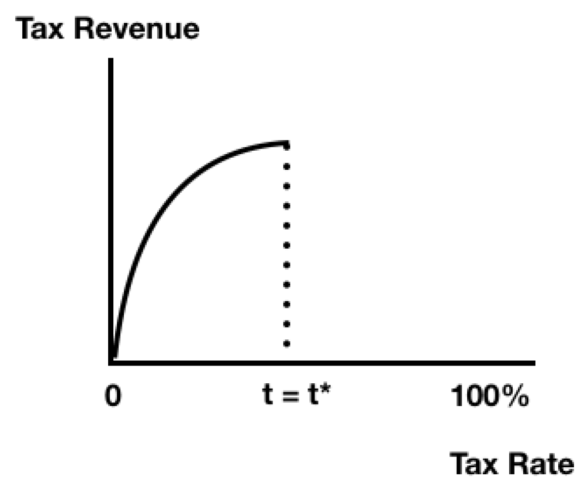
Case 2
Figure 3 presents a situation where t = t*. The possible utility from the leisure option is high enough to attract consumers out of the labor supply at a relatively lower tax rate that in Case 1. In this case, the declining portion of the Laffer curve cannot be identified. For the current experiment the first case with t < t* can be identified based on the fairness model and the experimental data. Moreover, in a society with a continuum of heterogeneous individuals, some of whom having very low utility of outside options, the aggregate tax revenue could still be fully continuous and exhibit the traditional Laffer curve as shown by Case 1.
For representative consumer opting to work (x > 0), substituting Equation (1) into the tax revenue formula gives;
The FOC for the revenue maximization is:
The details of FOC calculation are reported in Appendix D. The functional form for the perceived unfairness about the tax rate is assumed to be linear and is given by the equation: where beta captures the perceived unfairness of the participants regarding the tax and is positive. This functional form has been assumed to keep the model simple and find an explicit (closed form) solution for the observance of the Laffer curve based on the values of alpha and beta parameters. A more complex PF(t) function would make the model more complicated, and leave too many parameters to estimate.
Using in Equation (3), we get the following revenue maximizing condition.
For the Laffer curve to exist at ,
If
If
For the Laffer curve to exist the magnitude of the disutility arising from the work done measured by the parameter alpha () as well as the perceived unfairness about the tax captured by the parameter beta () are important. If these two variables are large enough, then the participants will decrease the labor supply to an extent where the tax revenue starts decreasing after a certain tax rate. If these parameters are very small, then no matter how large the tax rate is, the participants will not decrease the labor supply to an extent where the Laffer curve could show up.
The value of alpha has been estimated from Equation (1). Non-linear estimation has been used to estimate the value of alpha. The value of beta has been estimated from the equation .
Based on our previous analysis we can state the following testable hypotheses.
Hypotheses 1.
The declared number of tasks under the strategy method will be similar to the ones solved under the direct method.
Hypotheses 2.
Perceived unfairness of tax has a significant influence on the decision maker’s utility and hence the labor supply as well.
Hypotheses 1 is derived from the literature, which predicts that, if participants have completely correct understanding about their abilities and effort costs in solving the experimental tasks, both methods would lead to identical results in the lab [10]. Hypothesis 2 is based on the fairness model and it states that perceived unfairness about the taxation will influence the utility as well as the labor supplied by the consumers. If the value of beta () is significant, it will provide evidence in the favor of Hypotheses 2.
5. Results
5.1. Productivity across the Methods
There is no significant tax ordering effect observed under the direct method treatment. Hence, data for the increasing and decreasing tax rounds has been pooled together. Only one participant opted for the leisure option at a tax rate of 85% under the strategy method while no participant opted for the leisure option under the direct method treatment. For the participant opting for the leisure option, (Figure 3). Five (8.8%) of participants in the strategy method treatment were unable to complete the declared number of tasks during the specified time and hence their earnings for the correctly solved tasks were reduced to half.
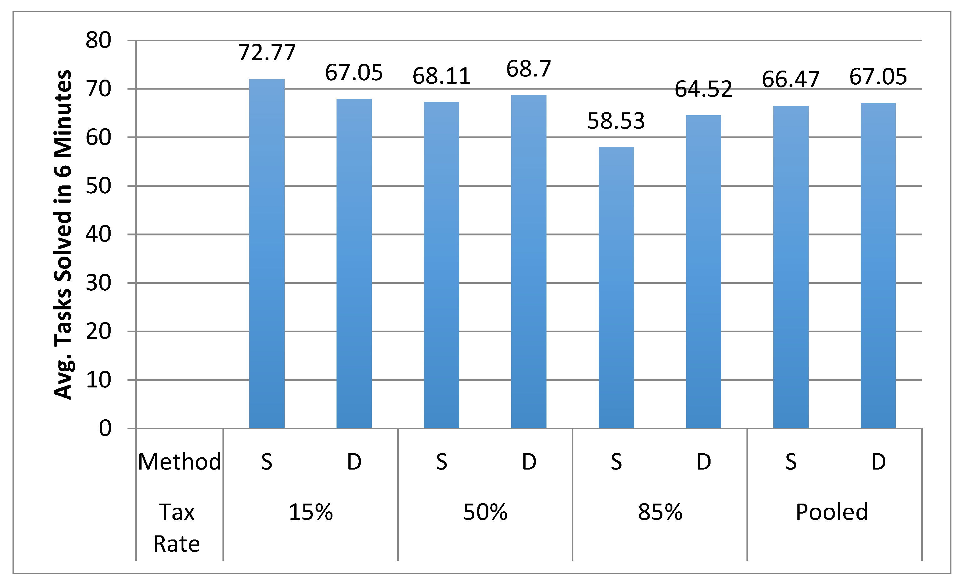
Figure 4 reports the average number of tasks solved for the direct and the strategy methods at three tax rates. It also reports the average tasks solved for the data pooled for the three tax rates.
The data pooled for the tax rates indicate average productivity under the strategy method treatment is 65.71 tasks per 6 min while it is 67.05 tasks per 6 min under the direct method treatment. Both parametric (t-test) and non-parametric (Mann–Whitney test) confirm no significant difference in these average productivities. Similarly, at 15%, 50% and 85% tax rates, there are also no significant productivity differences across the two methods (p < 0.05). Hence, there is not enough support for rejecting the Hypotheses 1. The possible reasons for this outcome are explored in Section 6 Table 2 reports these productivity comparisons among the methods.
5.2. Fairness Adjusted Laffer Curve Based on
Table 3 reports the estimates for alpha and beta for the strategy and the direct methods along with data pooled for both the methods.
The values of alpha for both methods are significant (p < 0.01) and also identical (0.02). The values for beta are also significant (p < 0.01) for both methods and are statistically identical as well. A higher beta estimate means the perceived unfairness about the tax rate is higher. The relatively higher value of beta in the current study can be related to the poor performance of the successive governments in Pakistan and their inefficient use of the tax revenues. In Pakistan, 60% of the people are not satisfied with the performance of the government [18]. A higher proportion of dissatisfied people in Pakistan are the primary reason we have a relatively higher value for beta parameter. The significant value of beta also provides support for the Hypotheses 2, indicating the utility as well as labor supply decisions are influenced by perceived unfairness of taxes.
The value for for both the direct and the strategy methods as well as for the pooled data satisfies the condition and we have for 15% and 50% tax rates. However, for 85% tax rate, the inequality gets reversed indicating a decline in the tax revenues. The value for for the pooled data is 0.1, and the corresponding revenue maximizing tax rate turns out to be 54%. Hence, according to the model, the declining revenue should start once the tax rates are higher than 54%. The revenue maximizing tax rate for the strategy and the direct method also turns out to be 54% based on their and estimates. The Laffer curve does not have to be symmetric (peaking at 50% tax rate for the current case). Even the original paper by Laffer [2] does not specify a symmetric shape of the Laffer curve. Hence, the asymmetric Laffer curve with revenue maximizing tax rate to be 54% is in line with the theory of the Laffer curve. If we connect the three revenue points against the three tax rates used in the experiment, the asymmetric behavioral Laffer curve will be suppressed. Since the fairness model shows the tax revenue gets maximized at a tax rate of 54%, it is possible to have higher revenue at 85% tax rate as compared to 50% and still get the Laffer curve. This asymmetric Laffer curve based on the estimated values of alpha and beta shown in the Figure 5.
The revenue for 50% tax rate, as shown in Figure 2, is lower than the revenue for 85% tax rate, but still there is a Laffer curve peaking at 54%. The goal of the fiscal policy makers is to maximize the tax revenue while taking care of the welfare of the society. The behavioral model shows the revenue maximizing tax rate to be 54% while the analysis based solely on the tax rates and tax revenues shows 85% to be the revenue maximizing tax rate. A tax rate based on the simple relation of the tax rates and the tax revenues can underestimate its impacts on the labor supply and welfare of the workers. Hence, to formulate an informed and robust policy, incorporation of behavioral elements, especially perceived unfairness of the taxes, in the traditional Laffer curve theory is essential.
6. Discussions and Conclusions
Using controlled lab experiments, this study explored the Laffer curve and labor productivity under the direct and the strategy methods. The results show no significant productivity differences between the direct and the strategy methods. Participants on average solved 67.05 tasks in the direct and 65.71 tasks in the strategy method treatments. It means, if the participants have completely correct understanding about their abilities and effort costs in solving the tasks, the two methods would lead to identical results. Hence, Hypotheses 1 cannot be rejected. However, some of the possible limitations of the current implementation of the strategy method should be discussed. The declaration of the tasks in the strategy method seems to be a target to achieve. Setting a high target can be a powerful motivational tool in these types of tasks. Alternatively, subjects might work harder in the strategy method to avoid the loss of half of their earning, an incentive that will be particularly strong under loss aversion. Another possible reason can be the overconfident behavior of participants in declaring the maximum number of tasks they can solve. As Niederle and Vesterlund [19] reported, more often participants declare the strategies in the lab driven by overconfidence rather than being realistic, and hence we see a relatively high productivity in the strategy method. As there was a practice round in the strategy method to help participants form a belief about their productivity, it could have minimized the aforementioned limitations of the strategy method.
The traditional income–leisure tradeoff cannot always explain the absence of the Laffer curve in the experimental lab and does not predicts the possible effects taxes on the labor supply in a robust manner and hence this study tried to modify the Laffer curve theory by adding behavioral aspects to it. The paper specified a fairness model based on the perceived unfairness of taxes and the disutility of work predicting a Laffer curve with revenue peaking at 54% tax rate for the current experimental data. The beta parameter capturing the perceived unfairness of tax is significant indicating these preferences do influence the supply of labor and hence the tax revenue. In addition, if it means PF(t) does not influences the utility function and hence the labor supplied as well. The value of beta has been tested for all three possible tax rates and has been found to be significantly different from (p < 0.01). Both results indicate PF(t) does influences the utility as well as labor supply decisions. Hence, there is clear support for Hypotheses 2. Public policies makers try to maximize the tax revenue while taking care of the welfare of the labor force as well. A policy based on the relation between the tax rates and tax revenues can lead to too high tax rates and discourage the labor supply. For an effective and publicly acceptable tax policy, the use of the proposed fairness adjusted Laffer curve can better serve the purpose.
The paper makes several important contributions to the existing literature. The first contribution is it compares the Laffer curve and human productivity under the direct and the strategy methods. To the best of my knowledge, this paper is the first one in the Laffer curve literature to make such a comparison and can be very helpful to the future research in this field. As another, probably more important, contribution, this paper provides a new dimension to the Laffer curve theory by specifying a Laffer curve based on the behavioral elements of perceived unfairness of taxes and the disutility of work. The proposed fairness adjusted Laffer curve can work equally well for both exogenous and endogenous taxes.
This paper compares the Laffer curve and productivity under the direct and the strategy methods using exogenous taxes. Future research making this comparison using endogenous taxes is needed to further enrich the experimental literature on the Laffer curve and identify if the two methods lead to same results or not.
Supplementary Materials
The following are available online at https://www.mdpi.com/2073-4336/9/3/56/s1, the supplementary materials including experimental instructions, zTree programs and dataset.
Author Contributions
All the work related to the data collection, model formation and writing the paper is done by the author (H.U.) himself.
Funding
This research received no external funding.
Conflicts of Interest
The authors declare no conflict of interest.
Appendix A. Survey Question about Perceived Unfairness of Tax
The perceived unfairness of tax was measured by asking the following question to the participants at the end of the experiment:
Rate the following tax rates that were used in the experiment on an unfairness scale of 1 to 5, where a higher value means more unfair the tax rate.
- (a)
- 15% (1 2 3 4 5)
- (b)
- 50% (1 2 3 4 5)
- (c)
- 85% (1 2 3 4 5)
Appendix B.
Bolzano’s theorem
f(t) can be non-negative at t = 0 depending on the value of alpha and PF(t). As the value of PF(t) is defined from the post experimental survey, we only need to specify the limits on the value of alpha for f(t) to be non-negative at t = 0.
For to be non-negative, . Solving this, we get:
As long as the estimated value of , and the Bolzano’s theorem will hold giving a t*. The value of alpha estimated from the experimental data turns out to be 0.052, while the maximum value that PF(t) can take is 5. Hence , which is significantly less than 0.4.
is clear from the function itself. Hence, satisfies the Bolzano’s theorem.
Appendix C.
FOC for the participation constraint
Appendix D.
FOC for the revenue function.
The FOC for the revenue maximization is:
References
- Khaldun, I. The Muqaddimah of Ibn Khaldun: An Introduction to History; Franz, R., Translator; Princeton University Press: New York, NY, USA, 1958; Available online: https://asadullahali.files.wordpress.com/2012/10/ibn_khaldun-al_muqaddimah.pdf (accessed on 21 June 2018).
- Laffer, A.B. Backgrounder No. 1765: The Laffer Curve: Past, Present and Future; The Heritage Foundation: Washington, DC, USA, 2004; Available online: https://www.heritage.org/taxes/report/the-laffer-curve-past-present-and-future (accessed on 21 June 2018).
- Sutter, M.; Hannemann, H.W. Taxation and the veil of ignorance—A real effort experiment on the Laffer curve. Public Choice 2003, 115, 217–240. [Google Scholar] [CrossRef]
- Garboua, L.L.; Masclet, D.; Montmarquette, C. A behavioral Laffer curve: Emergence of a social norm of fairness in a real effort experiment. J. Econ. Psychol. 2009, 30, 147–161. [Google Scholar] [CrossRef] [Green Version]
- Robert, M.; Lyle, D.C. Public confidence and admitted tax evasion. Nat. Tax J. 1986, 37, 489. [Google Scholar]
- Alm, J.; Jackson, B.; McKee, M. Fiscal exchange, collective decision institutions, and tax compliance. J. Econ. Behav. Organ. 1993, 22, 285–303. [Google Scholar] [CrossRef]
- Andreoni, J.; Erard, B.; Feinstein, J. Tax compliance. Am. Econ. Assoc. 1998, 36, 818–860. [Google Scholar]
- Cornelissen, T.; Himmler, O.; Koenig, T. Fairness spillovers-The case of taxation. J. Econ. Behav. Organ. 2013, 90, 164–180. [Google Scholar] [CrossRef]
- Martinez, L.P. The trouble with taxes: Fairness, tax policy and the constitution. Hastings Const. Law Quart. 2004, 31, 413. [Google Scholar]
- Brandts, J.; Charness, G. The strategy versus the direct-response method: A first survey of experimental comparisons. Exp. Econ. 2011, 14, 375–398. [Google Scholar] [CrossRef] [Green Version]
- Keser, C.; Masclet, D.; Montmarquette, C. Labor supply and redistribution, a real-effort experiment in Canada, France and Germany. In Clrano Working Paper; Center for Interuniversity Research and Analysis of Organizations: Montreal, QC, Canada, 2015. [Google Scholar]
- Ottone, S.; Ponzano, F. Laffer curve in a non-Leviathan scenario: A real-effort experiment. Econ. Bull. 2007, 3, 1–7. [Google Scholar]
- Swenson, C.W. Taxpayer behavior in response to taxation: An experimental analysis. J. Account. Public Policy 1998, 7, 1–28. [Google Scholar] [CrossRef]
- Fochmann, M.; Weimann, J.; Blaufus, K.; Hundsdoerfer, J.; Kiesewetter, D. Net wage illusion in a real-effort experiment. Scand. J. Econ. 2013, 115, 476–484. [Google Scholar] [CrossRef]
- Hayashi, A.T.; Nakamura, B.K.; Gamage, D. Experimental evidence of tax salience and the labor-leisure decision: Anchoring, Tax aversion, or complexity? Public Financ. Rev. 2013, 41, 203–226. [Google Scholar] [CrossRef]
- Fischbacher, U. z-Tree: Zurich toolbox for ready-made economic experiments. Exp. Econ. 2007, 10, 171–178. [Google Scholar] [CrossRef] [Green Version]
- Mattsson, L.G.; Weibull, J.W. Probabilistic choice and procedurally bounded rationality. Games Econ. Behav. 2002, 41, 61–78. [Google Scholar] [CrossRef]
- Gallup Pakistan. Available online: http://gallup.com.pk/majority-pakistanis-are-not-satisfied-with-the-performance-of-government-federal-and-provincial-in-ending-corruption/ (accessed on 21 June 2018).
- Niederle, M.; Vesterlund, L. Do women shy away from competition? Do men compete too much? Q. J. Econ. 2007, 122, 1067–1101. [Google Scholar] [CrossRef]
Figure 1.
Work–leisure utility tradeoff.
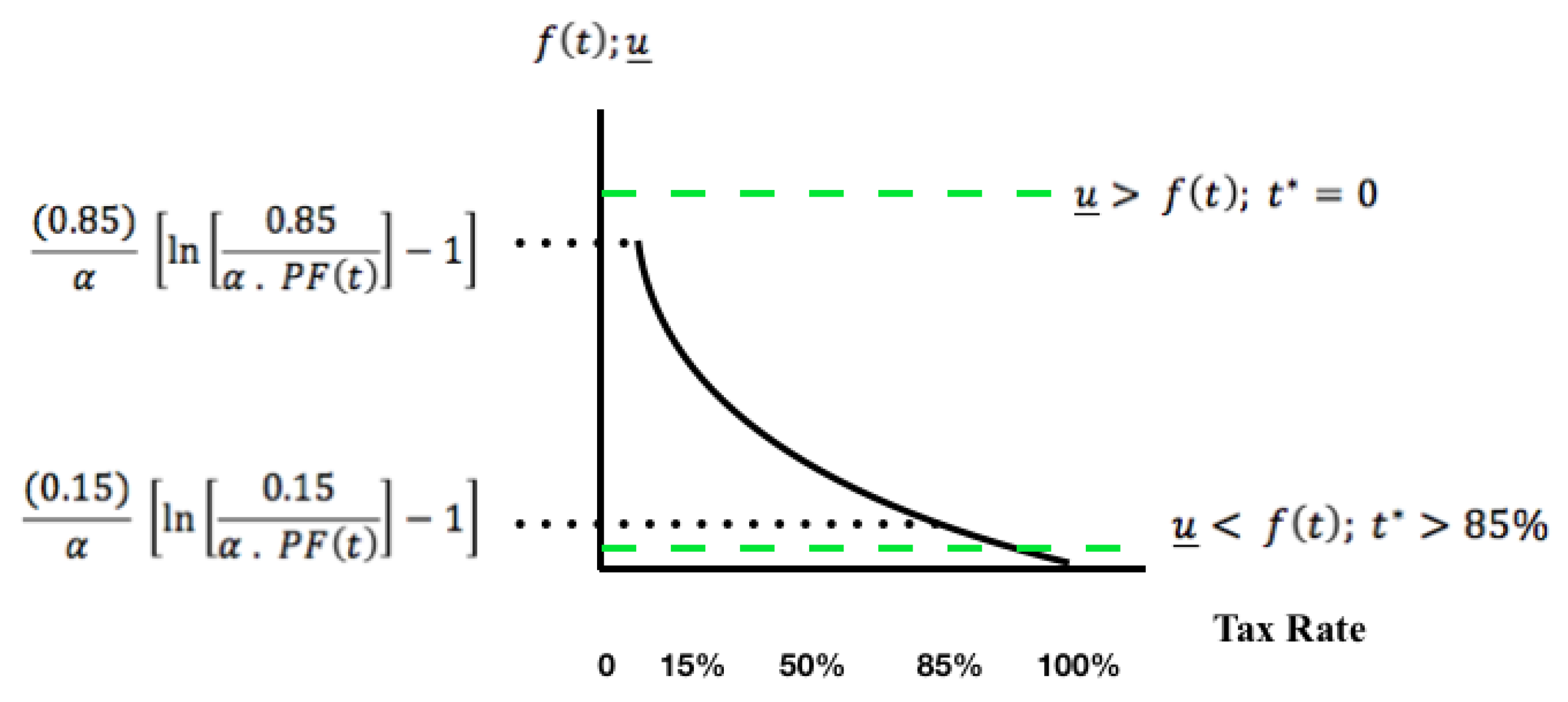
Figure 2.
t < t*.
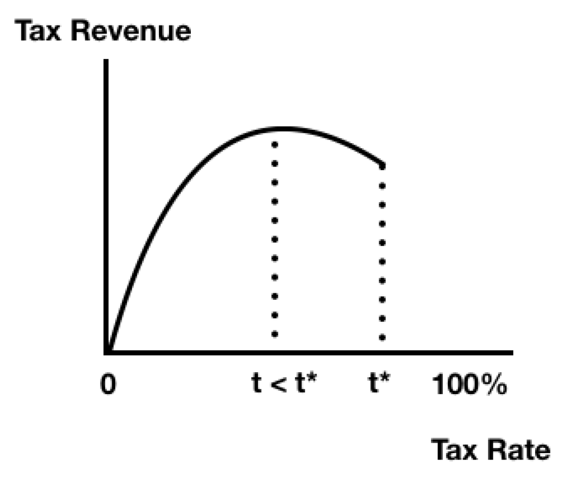
Figure 3.
t = t*.

Figure 4.
Average Productivity: Strategy versus Direct Method. S, Strategy Method; D, Direct Method.
Figure 4.
Average Productivity: Strategy versus Direct Method. S, Strategy Method; D, Direct Method.

Figure 5.
Asymmetric Laffer curve.


Table 1.
Regression Results for Laffer curve Estimation.
| Dependent Variable | Tax Revenue |
|---|---|
| 367.73 *** | |
| (17.27) | |
| −424.23 *** | |
| (20.99) | |
| Observations | 333 |
| R-squared | 0.63 |
Robust standard errors are in parentheses. *** p < 0.01.
Table 2.
Productivity Differences between the Direct and the Strategy Method.
| Tax Rates | Pooled Data | |||
|---|---|---|---|---|
| 15% | 50% | 85% | ||
| Avg. Tasks | S = 72.77 D = 67.05 | S = 68.11 D = 68.70 | S = 58.53 D = 64.52 | S = 66.47 D = 67.05 |
| z-Stat | 0.02 (0.98) | 1.06 (0.29) | 1.62 (0.10) | 1.63 (0.10) |
| t-Stat | 0.72 (0.48) | −0.30 (0.76) | −1.40 (0.17) | −0.18 (0.86) |
Note: S, Strategy Method; D, Direct Method. z-stat was obtained from the Mann–Whitney test while the t-stat was obtained from the Test of Means. p-Values are in parentheses.
Table 3.
Estimates of Alpha and Beta.
| Strategy | Direct | Pooled Data | |
|---|---|---|---|
| Alpha | 0.02 *** | 0.02 *** | 0.02 *** |
| R-Squared | 0.634 | 0.687 | 0.658 |
| Observations | 171 | 162 | 333 |
| Beta | 5.26 *** | 5.54 *** | 5.40 *** |
| R-Squared | 0.806 | 0.841 | 0.823 |
| Observations | 171 | 162 | 333 |
*** p < 0.01.
© 2018 by the author. Licensee MDPI, Basel, Switzerland. This article is an open access article distributed under the terms and conditions of the Creative Commons Attribution (CC BY) license (http://creativecommons.org/licenses/by/4.0/).
Share and Cite
MDPI and ACS Style
Umer, H. Fairness-Adjusted Laffer Curve: Strategy versus Direct Method. Games 2018, 9, 56. https://doi.org/10.3390/g9030056
AMA Style
Umer H. Fairness-Adjusted Laffer Curve: Strategy versus Direct Method. Games. 2018; 9(3):56. https://doi.org/10.3390/g9030056
Chicago/Turabian StyleUmer, Hamza. 2018. "Fairness-Adjusted Laffer Curve: Strategy versus Direct Method" Games 9, no. 3: 56. https://doi.org/10.3390/g9030056
Note that from the first issue of 2016, this journal uses article numbers instead of page numbers. See further details here.