To Tender or Not to Tender? Deliberate and Exogenous Sunk Costs in a Public Good Game


1
Tilburg Institute of Governance, Tilburg University School of Economics and Management, P.O. Box 90153, 5000 LE Tilburg, The Netherlands
2
School of Economics, Faculty of Social Sciences, University of Nottingham, Nottingham NG7 2RD, UK
*
Author to whom correspondence should be addressed.
Games 2018, 9(3), 41; https://doi.org/10.3390/g9030041
Submission received: 25 May 2018
/
Revised: 15 June 2018
/
Accepted: 22 June 2018
/
Published: 26 June 2018
(This article belongs to the Special Issue Public Good Games)
Abstract
:In an experimental study, we compare individual willingness to cooperate in a public good game after an initial team contest phase. While players in the treatment setup make a conscious decision on how much to invest in the contest, this decision is exogenously imposed on players in the control setup. As such, both groups of players incur sunk costs and enter the public good game with different wealth levels. Our results indicate that the way these sunk costs have been accrued matters especially for groups on the losing side of the contest: Given the same level of sunk costs, contributions to the public good are lower for groups which failed to be successful in the preceding between-group contest. Furthermore, this detrimental effect is more pronounced for individuals who play a contest with deliberate contributions before.
1. Introduction
In economics and in society in general, many situations are of a competitive kind. For example in public tenders, (cellular telephone) license lotteries or struggles for resources, considerable funds are spent to outperform a competitor. One of the most widely used models for (team) competition is the contest game [1,2], where agents invest resources in order to influence the probability to win a prize.
In the field, however, the factual rents derived from the prize at stake are often not fully defined ex ante and depend on what the winning party makes of it. Ref. [3] presents a model for an endogenous contest prize, in which players’ contributions determine both the probability of winning and the value of the prize. By contributing to the contest, players create a positive externality to all other competitors by increasing the prize at stake. At the same time, contributing generates negative externalities, as it reduces other players’ probability to win. As economic application, consider a situation where R&D efforts affect realised profits from having the best idea.
However, contributions to winning the contest often do not directly influence the variable prize at stake. This is determined separately from the contest instead. Imagine a procurement tender for a construction project involving two corporations—each consisting of several subdivisions—running for the contest. After the decision on which one has been awarded with the project, the subdivisions of the winning corporation can deliver input to construct the project of which the benefits are shared equally within the winning corporation.
A related example of this kind of contest is the recent competition between Boeing and Airbus for a major deal with El Al Airlines.1 We depart from the standard conceptualisation of this market situation as duopoly of unitary players towards a more complex (and probably more realistic) one. As such, each competitor consists of different segments (for the aviation example e.g., production of fuselage, wings, turbines) and eventual rents depend on success or failure in the competition and the subsequent behaviour of each firm’s segments, under incomplete contracts. Our model also applies to situations in which the group’s payoff depends on their relative performance within an organisation (i.e., R&D units, independent profit centres).
There are two stages: First, on the corporation level, each group spends resources to secure the project. In the second stage, subdivisions invest resources for a project, whose benefits are shared equally within the firm. Both firms produce after the contest, but we assume that the successful group managed to gain access to a more attractive project, delivering higher returns on capital.2 Theoretically, contribution decisions to the group project—which constitutes a public good—should be independent of the amount of money spent in the first stage, as it represents a sunk cost. Literature suggests though, that agents’ decisions are in fact influenced by sunk costs [7]. More specifically, individuals seem to be more willing to invest into an ongoing project, if more money has been spent on it before e.g., [7,8].
Subdivision managers in charge could as well be subject to the inverse effect, though. Contributing to the tender could be perceived as the first stage of a reciprocal or gift exchanging process. As such, having invested a lot of resources in the first stage could make individuals feel entitled to cut back for the public good. Another argument for this behaviour would be inequity averse preferences (cf. [9]), as those who contributed more to the first stage of the game are relatively poorer. So far, research on sunk cost has mainly focussed on investment or consumption decisions. However, the dynamics of a public good game with a prior investment decision are different, because social preferences (as for example, reciprocity) have a bearing on decision making as well.
In this paper we present an experimental study to investigate the effect of a first-stage investment on agents’ willingness to contribute to a public good. Furthermore, the experimental design allows to disentangle the effect of unintentional exogenous sunk costs from sunk costs emanating from deliberate investments into a between-group contest. Executing this study in a controlled laboratory setting allows isolating aforementioned factors and to draw more robust conclusions.
The article is structured as follows: In the next section we discuss the conceptual background of our study; then we explain the setup of the experiment in Section 3; in Section 4 we formulate hypotheses; before presenting results in Section 5; Section 6 provides concluding comments and suggestions for future research.
2. Background
This article draws from three different strands of literature:
- Endogenous prize contests,
- Public good games with entry option and
- Sunk costs
In this section we review some of the relevant literature.3
2.1. Endogenous Prize Contests
An important component of contests is the prize at stake (cf. [12,13]). Not only does it represent the motivational cue for engaging in a contest from a behavioural perspective, but it also determines the equilibrium prediction in pure strategies (cf. [13,14]). In the field, there exists several contest situations with an exogenous prize, like a money prize in sports tournaments or known rents from patents in R&D races. However, often the contestants themselves can influence the prize to take away from a successful competition. So far research on endogenous contest prizes has focused on scenarios where the prize is influenced by players’ contribution to the contest [3,15] or by the price demanded in a Bertrand competition game [4,16].
In [17], participants were able to make a real-time decision on entering a contest, while observing the number of co-players currently in the market. They find a substantial excess entry into the market, as compared to the risk neutral benchmark prediction. This was especially the case when the outside option underlay a stochastic risk. The symmetric equilibrium investment level in the subsequent contest negatively depends on the number of entrants into the market. While [17] join the ranks of articles that find considerable overspending into the contest, they also observe a large fraction of participants exhibiting a rather passive investment strategy after having decided to enter the contest. Ref. [17] offer two explanations for the behaviour of this latter group:
- Escape the outside option for treatments where it is risky.
- Risk or loss averse individuals entering the market early, under the expectation that only few other players would enter, refrain from placing a high bid upon observing that there were in fact unexpectedly many entrants to the market.
Ref. [18] conduct an experiment where players auction for the right to participate in a coordination game. The price for the right to play reduces strategic uncertainty and works as a tacit communication device. While participants consistently fail to coordinate on a payoff-dominant equilibrium when endowed with the right to play, those who went through a pre-play auction, achieve the efficient outcome in the coordination game.
In the context of a weak link game, Ref. [19] compare a market mechanism with random sorting with regards to players’ productivity. While there exists an efficiency gain from the market mechanism for high performance workers, this effect is almost completely offset by a negative effect on players with low performance pay.
We present an endogenous contest prize where the contributions for outperforming the competitor do in fact not influence the size of the prize. Instead, these expenses are dedicated solely to the contest. Public tenders, for example, are widely used for determining the granting of funds for projects or for (public) facilities. Success or failure of the project depend on the winning party’s behaviour in the post-contest phase.
2.2. Public Good Games with Entry Option
There exists an established theoretical literature on public goods games with entry option. Refs. [20,21] argue that when individuals can opt between setting up a partnership with another player or an outside option, entering conveys a message about the players’ types. This helps coordination towards more efficient, cooperative strategies. Other authors refer to a false consensus bias as the reason for the matching of types. If this is the case, cooperators are relatively more likely to enter the cooperative game, as they tend to be more optimistic about the level of cooperation, than free riders are [22].
Refs. [23,24] examine the effect of voluntary entry to a public goods game experimentally. Ref. [23] find a positive effect on cooperation and efficiency in the presence of voluntary entry to a one-shot public goods game. Ref. [24] compare the effectiveness of an entry option with an exit option in a one-shot public goods game experiment. Although the possibility to exit increases the ability to coordinate towards the cooperative strategy, the entry option does not deliver a significant effect.
2.3. Sunk Costs
Classical examples of elicitation of sunk cost fallacies or escalating commitment, demonstrate cases where agents are more willing to invest (additional) resources with higher previous investments [7,25]. One field study reported in [7], for example, demonstrates that individuals who paid the full price for a theatre season ticket attend more performances than those who have randomly benefited from a reduced price. Among the most prominent psychological explanations for the sunk cost fallacy is prospect theory [26]: People do not update their reference point which makes them accept too much risk. Ref. [27] offers a self-justification bias as alternative explanation: Individuals tend to invest more resources into a losing asset in order to rationalise or justify their previous strategy.
One prominent aspect of our design is the fact that we can contrast sunk costs incurred exogenously and those having been accrued deliberately by the player herself. So far, most existing evidence on this topic is based on data where the sunk costs have either been exogenously defined by the experimenter i.e., [25] or endogenously accrued by the player i.e., [28].
An example that considers this issue is presented by [29]. In an experimental study they examine the effect of auctioning entry rights to a market on subsequent prices. In one treatment, agents do not issue bids themselves, but entry rights are given randomly and the same cost as in the auctioning treatment is induced exogenously. Most notably, prices do not differ between the auction and the exogenous treatment. At the same time, the effect size of the sunk cost fallacy seems to depend on the market situation. While there is a significant positive effect on average prices in an oligopolistic market, they are unaffected in the monopoly treatment. Ref. [29] argue that while the entry fee encourages players to risk engaging in a collusive strategy, this was—by design—much less of an issue in the monopoly market because collusion is not possible by definition.
3. Setup
Before the main part of the experiment, we take a measure of individual social value orientation (SVO), using techniques introduced by [30].4 We would expect players with a higher SVO score (i.e., more prosocial types) to exhibit a greater willingness to contribute to the group project, as second stage contribution is socially beneficial. Ref. [31] conduct a meta-analysis studying the effect of SVO on cooperation in social dilemma games, employing 82 effect sizes from individual studies. Overall, they find a “small to moderate (positive) relationship between SVO and cooperation in social dilemmas”, with the underlying effect being most robust in public goods dilemmas. Conceivable hypotheses concerning first stage expenditures are less obvious. An argument could be made that more competitive types (i.e., those with a very low SVO score), spend more resources in a competitive game like our between-group contest. Additionally, if more socially oriented participants recognise the overall welfare reducing character of the between group contest, this should drive out first stage expenditures from higher SVO score-types.
This study incorporates two experimental treatments: A competition treatment and an exogenous treatment. While subjects in the former treatment compete for the right to play a public good game with a relatively more attractive Marginal Per Capita Return (MPCR), players in the latter treatment incur an exogenous cost, before being sorted into an either high or low MPCR game. Details are described in what follows.
[Competition treatment:] Players are sorted in groups of three and compete against another group of the same size. This composition keeps unchanged and players’ identities are never associated with their decisions. The game consists of two stages and it includes investment decisions as explained in the following.
- First stage
- Each player receives an endowment of tokens. For a price of 1 token per ticket, they can purchase up to 100 tickets for the contest. Spendings of subject k in group K and m in group M are labelled and , respectively. Tokens that are not spent for the contest will be added to the player’s private account. With being the probability for group K to win over group M, the contest success function (CSF) similar to [1,2] is
- Second stage
- Players learn if their group has won or lost, other group’s first stage spending level, the corresponding winning probability and their group mates’ wealth level . Then, each group plays a public good game with being individual i’s investment into the public good.5 For this, subjects can invest a maximum of 100 tokens.6 The winning group will enjoy a high MPCR of . The losing group will be facing a low MPCR of .7 Individual payoff is then determined by:
[Exogenous treatment:] Players are sorted in groups of three and are connected with another group of three, analogous to the competition treatment. Their first stage behaviour will be matched with a pair of groups in the competition treatment. This means, for each pair of groups with voluntary first stage spending, there will be a pair of groups in the exogenous treatment, that gets the same amount of tokens deducted by the computer.8 Participants pass the following two stages:
- First stage
- Each player receives an endowment of tokens. Individual factors are induced, matching another group’s behaviour in the competition treatment and deducted from T.
- Second stage
- Groups play a public good game. Players see the current wealth level of their group mates (being ) and the wealth level of the other group they are connected with. Keeping in line with the matched groups from the competition treatment, the MPCR will be or . Individual payoff is determined by:
Procedures
Using ORSEE by [32] we recruited 186 participants for the experiment, which was conducted in the CeDEx lab at the University of Nottingham between May 2015 and March 2016. During this computerised laboratory experiment,9 each participant sat in a cubicle, visually separated from each other. Participants were randomly seated at one of 24 computers and found the instructions for the SVO measure at their place. After the SVO measure was taken, instructions for the main part were distributed. All instructions were read aloud both in order to enhance the understanding and to make it credible to the participants that everyone shares the same information.10
The main part of the experiment started with a thorough trial period, including comprehension questions, in order to make participants familiar with the interface and to ensure an accurate understanding.11 After the main part, participants answered a short questionnaire about personal attributes (i.e., age, gender) and preferences (political convictions, risk attitudes...).
The experiment took one hour, which included reading instructions, taking an SVO measure, a trial period, the main part of the experiment, a questionnaire and payment. Average earnings were £12.00, which was paid out privately and in cash at the end of the session.12
4. Hypotheses
First, we present predictions under standard assumptions in Section 4.1. Afterwards, we discuss alternative hypotheses, first on group level in Section 4.2. Lastly, in Section 4.3 we turn to the individual level, presenting the competing Hypotheses 4–6.
4.1. Standard Predictions
Under risk-neutrality and individualistic preferences, each player i in group K maximises her expected earnings, which is
As , investment into the public good is socially desirable but individually costly for risk-neutral individualistic agents, who are only concerned with their own earnings. The second-stage Nash equilibrium therefore is , which renders both public good games indifferent in expected values, i.e., zero. In the competition treatment, no resources will be spent in the first stage, so . Find a more formal approach in Appendix B.
Hypothesis 1.
Risk-neutral and individualistic players will contribute 0 in both stages of the game.
4.2. Behavioural Hypotheses—Group Behaviour
Next to the subgame perfect equilibrium as benchmark we formalise alternative hypotheses to capture other regarding preferences.
Hypothesis 2.
Winning groups will spend more for the team project than losing groups.
Hypothesis 3.
The difference in spending levels for the team project will be more pronounced for the competition treatment.
More specifically, Equation (1) formalises these hypotheses concerning the relation between the different mean contribution rates for each possible second stage outcome.
represents average contribution levels given a particular group has won or lost (i.e., , respectively) and given the group is in either the competition or the exogenous treatment (i.e., , respectively).
The second inequality (between winning and losing groups) is in line with established empirical results on public good games, that contributions increase with higher MPCR e.g., [34,35,36]. For the first and the last inequality, we expect this tendency to be more pronounced for the competition treatment because of sorting and signalling effects. Using first stage contribution, players can signal their other-regarding preferences, i.e., players who spend resources to win in the first stage have more cooperative dispositions.
Two alternatives would be:
- Groups end up winning the contest because they have more competitive players, or
Using the SVO score we can test which explanation prevails. Under behavioural spillovers, a player’s SVO would have no effect on first stage contribution.
4.3. Behavioural Hypotheses—Individual Behaviour
Applying a forward looking argumentation as in [39], the size of first stage contributions conveys a signal about future play. To make an investment of in the first stage of the competition treatment, a player expects her profits in stage two to be at least higher than without this prior investment. This reduces strategic uncertainty, as players can eliminate from consideration the set of strategies, that are payoff dominated in this sense. Ref. [39] offers an alternative argument for why first stage contribution could trigger higher cooperation to the team project. In their theoretical model, “players forecast how the game would be played if they formed coalitions and then they play according to their most optimistic forecast” [39]. If first stage spending is interpreted as signal towards the level of cooperativeness, this can make the “most optimistic forecast” more viable, increasing the likelihood of it being played. This reasoning does not apply when players incur sunk costs randomly. First stage sunk costs in the exogenous treatment do not convey a tacit signal about players’ types.
Hypothesis 4.
Players who spend more in the team contest are also more cooperative in the public good game.
As discussed in Section 2.2, voluntary contribution to the first stage contest in our setup can be interpreted as an implicit signal about whether or not an agent intends to engage in the second stage public good game. Relating to the argument above, if cooperators are more optimistic about the level of cooperation, they estimate higher expected profits from the second stage public good game. Therefore we hypothesise that agents, exhibiting cooperative behaviour in the second stage, tend to spend more resources in the contest.
From this we derive a hypothesis concerning the relationship of second stage () and first stage contribution (), formalised in Equation (2) below:
Hypothesis 5.
More wealthy players spend more to the public good game.
Hypothesis 6.
This effect is more pronounced in the competition treatment.
By the nature of this game’s structure, participants might very well enter the public goods game with different wealth levels. Agents that have spent more resources in the contest are relatively poor and vice versa. At the same time, contributions to the second stage public good are restricted to 100 tokens, irrespective of players’ first stage behaviour. Ref. [40] study the emergence of contribution norms in a public good game with heterogeneous agents. Without punishment opportunities, there is no significant difference in contribution to the public good between agents with different money endowment. This is the case despite (uninvolved) individuals’ stated normative preferences “that high types should contribute more”.13
If players are indeed motivated by inequality concerns in the sense of [9,44], more wealthy agents—those with lower first stage spendings—would contribute relatively more in the second stage. Accordingly, Hypothesis 5 is antithetical to Hypothesis 4 and we would observe a negative relationship between second stage contribution and first stage spending level of a player—i.e., the opposite of Equation (2). Our setup allows to disentangle inequality concerns from actions motivated by reciprocity. It is only in the competition treatment that first stage contributions are determined by a conscious decision from the respective player. Accordingly, the relationship between first stage contribution and second stage spending would only exist in the competition treatment if contributions to the team project are motivated by reciprocity.
5. Results
This section consists of three parts. First (Section 5.1) we describe the contest spending behaviour in the competition treatment. We analyse, which individual factors determine the willingness to spend resources to the between group contest. In the second part (Section 5.2) we study how much participants contribute to the team project and discuss structural differences comparing winning and losing groups for the two treatments. Afterwards, we investigate the relationship of first and second stage contribution (Section 5.3 and Section 5.4).
As this is a one-shot game, individual data can be tested as independent observations. For hypothesis testing, we use non-parametric methods, as the data is not normally distributed (Shapiro-Wilk test for normality. N = 186, P = 0.00. Same result for first stage and second stage contribution.): Wilcoxon signed-rank test (Wilcoxon test) for paired data [45] and Mann-Whitney U test (MWU) for independent sample data [46]. We test for trends using Spearman’s rank correlation (Spearman test) [47,48]. For regression analyses we employ a Tobit model with limits at 0 and 100, as this is where the action space is limited.14 All regressions (both Tobit and OLS) concerning second-stage behaviour apply standard errors that allow for intragroup correlation (as in, chapter 8) [49,50].
5.1. Team Contest
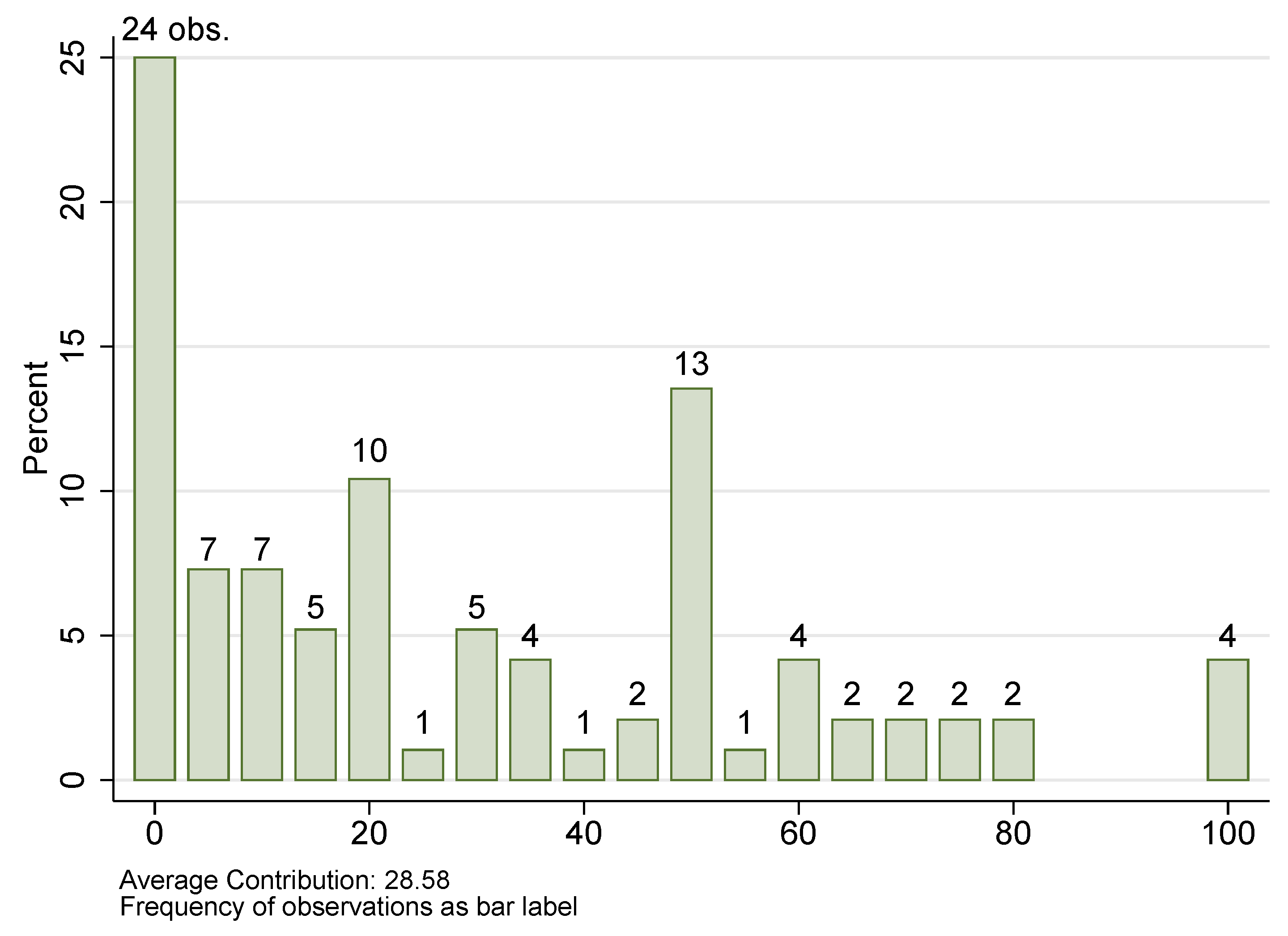
Participants spend on average about 29 points on first stage tickets, which is substantially higher than the benchmark prediction of zero contribution.15 Figure 1 depicts the distribution of team contest contributions, indicating 0 as the modal contribution level. See Appendix C for a discussion of the role of beliefs for contest expenditures in this game.
We use Tobit regression with limits at 0 and 100, to analyse determinants of individual contribution to the between group contest; results are summarised in Table 1.16 First of all, the individual measure of social value orientation (SVO)17 has a positive effect on the first stage contribution behaviour. This means that participants with a relatively more social orientation chip in with more resources for the between-group contest. Furthermore, the self-reported risk tolerance measure (risk parameter) has no explanatory power for how many lottery tickets are bought. In [2,14], by contrast, equilibrium contributions diminish with higher levels of both constant absolute risk aversion and constant relative risk aversion.
Further controls were generated by a post-experiment questionnaire. We discover a strong gender effect, such that female participants purchase significantly more lottery tickets. The magnitude of this factor is substantial, given that the entire decision space only ranges from . The strong positive magnitude of this factor might come as somewhat surprisingly, given an established literature on women’s lower level of competitiveness e.g., [51,52]. To our knowledge, this puzzling result is not paralleled by other studies on (group) contest games. However, first stage contribution can be interpreted as “a task that each member prefers that another member of the group undertakes” [53]. The authors find that in mixed groups, women volunteer twice as often as men to take over such tasks.
Players’ age is also positively related to first stage contributions. While the range of age in our sample only spans from 18–32, studies in sports literature employing a broader sample, indicate a negative relationship between age and competitiveness [54].
Some of the control factors, such as number of siblings, smoking, politics important18 and hard work have no descriptive power for first stage spending behaviour.
Another strong positive effect is displayed by trust in others,19 such that participants who express a higher level of trust contribute more to the contest. In this sense, contest expenditures could be seen as sacrifice for the group’s benefit, which can repay if a high level of cooperation will be realised in the subsequent second stage.
The factor income equality displays a negative coefficient in Regression (2). Individuals stated their proximity to which of the two following statements they feel closer on a scale from one to seven: “We need larger income differences as incentives for individual effort.”—“Incomes should be made more equal.” Accordingly, this factor aims at capturing individual preferences for either a steep or flat income curve. There is some indication as to that more equality-oriented participants exert less resources for the between group contest.
5.2. Second Stage Contribution
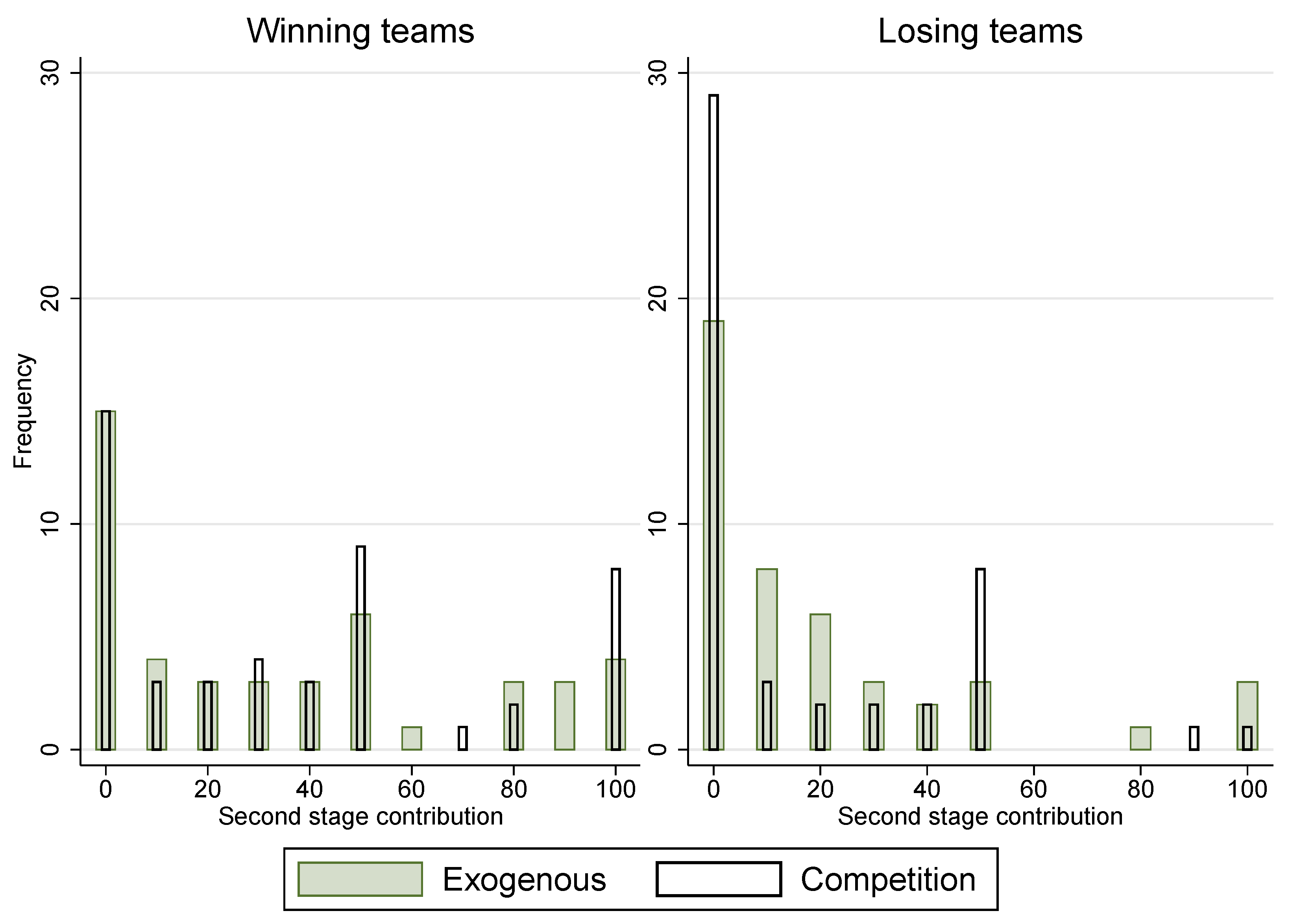
Table 2 lists average contributions for both treatments and winning and losing groups. Consider Figure 2 for an overview of individual contributions to the team project. Across all treatments and first stage outcomes, players invest on average about 27 points into the team project. Also notice that for the exogenous and the competition treatment, both average contribution levels are virtually identical overall. In Hypotheses 2 and 3 alongside Equation (1) we formulate three inequalities, reflecting differences in sorting and MPCR. As for the second inequality of our hypothesis, we observe a stark difference between average contribution levels comparing winning and losing teams, respectively (Wilcoxon test on team level: N = 62, P = 0.001. Higher rank sum than expected for winning teams). Members of the winning teams spend about twice as much on the team project, as compared to players in the losing teams. This is true for both the competition and the exogenous treatments.
The third inequality in our hypothesis postulates that players in a losing group in the competition treatment contribute less to the team project than a member of a losing group in the exogenous treatment. Although the average second stage contributions point in the right direction (19.5 for exogenous and 16.3 for competition treatment), non-parametric tests on the group level fail to back this hypothesis (Wilcoxon test on team level: N = 31, P = 0.566). At the same time, for losing groups complete free riding occurs much more frequently in the competition treatment (28 times) than in the exogenous treatment (19 times).
The results concerning the first inequality of Equation (1) pan out similarly: The underlying hypothesis states that individuals in a winning team contribute more in the competition treatment, as compared to winning teams in the exogenous treatment. While the average second stage contributions slightly tend towards this direction (34.3 for exogenous and 37.2 for competition treatment), this indifference is far from being significant (Wilcoxon test on team level: N = 31, P = 0.566). Hence, participants seem to not perceive contributions to the contest as a strong signal for second-stage cooperativeness in the winning groups.
5.3. Relation between First and Second Stage Contribution
Based on the argument that first stage contribution is used as costly device to signal the willingness to cooperate in the team project, we formulate Hypothesis 4 (Section 2.3 adds to this, applying a sunk costs argumentation), which postulates a positive relationship between individual contest expenditures and the subsequent investment into the team project. Concurrently, we discuss an antithetic perspective on this matter by devising Hypothesis 5. Here, both inequality aversion and reciprocity actually warrant a negative relationship between first and second stage contribution. Our setup allows us to analyse which of the above arguments prevail.
In Table 3 we present results for a Tobit model with limits at 0 and 100 with robust standard errors for intra-group correlation.20 We regress contributions to the team project on first stage expenses and various other factors, as discussed below.21 Overall results for Regressions (3) through (6) deliver evidence to support Hypothesis 4, displaying a positive interrelation between the two factors. This means that players who tend to spend more in the contest phase of the game, are also those who chip in relatively more resources to the subsequent team project.
Group Contribute Minus Self controls for the amount of lottery tickets of a player’s group mates. Here also a positive relationship prevails between first stage contribution of the others in a group and second the player’s contribution to the team project.
The degree of social value orientation (SVO) positively influences the willingness to cooperate in the team project. This seems in line with the argument that one would expect more socially oriented individuals to invest more into the group account.22
In all Regressions (3) through (6), we include a dummy variable for each of the four situations a participant could end up in (outcome dummy henceforth):
- Exogenous lose
- Player in the exogenous treatment in a group that lost in the first stage.
- Exogenous win
- Player in the exogenous treatment in a group that won in the first stage.
- Competition lose
- Player in the competition treatment in a group that lost in the first stage. This is the default in regressions (3) through (2).
- Competition win
- Player in the competition treatment in a group that won in the first stage.
In Regressions (5) and (6) we additionally interact the outcome term with First stage Contribute, which captures eventual heterogeneities between the outcomes in terms of first stage spending levels. In consonance with the hypothesis tests above, both Exogenous win and Competition win are significantly positive for almost all regressions, confirming that winning in the first stage leads to higher contributions to the team project. When controlling for heterogeneities in lottery tickets between outcomes in Regressions (5) and (6), the dummy for Exogenous lose is even significantly higher than the default, which is Competition lose. This last finding is particularly interesting in the light of the third inequality of Equation (1). When allowing for a heterogeneous effect of first stage spending on contributions to the team project, differences between these two outcomes can be identified.
While overall there exists a positive relationship between first and second stage contribution, the interaction effect in Regressions (5) and (6) identifies this to be significantly lower in the exogenous treatment. Indeed, using a Tobit model with limits at 0 and 100 and robust standard errors for intra-group correlation, we find no relationship between first and second stage contribution in exogenous win and even some evidence for a negative relationship in exogenous lose.23 We will investigate this matter more closely in the next subsection. The results in this subsection establish that in the competition treatment, players’ second stage behaviour is not consistent with inequality aversion or reciprocity; instead first stage spending is used as costly signalling device for the following team project phase. Furthermore, participants are only prone to a sunk cost fallacy under deliberate sunk costs, not if these have been incurred exogenously.
Furthermore, in Regressions (3) and (4) the intercept for Competition win is significantly higher than its counterpart from the losing situation, while the two slopes are about the same. This is some evidence that in the competition treatment, losing the between group contest pans out as constant drag on a group’s cooperation level towards the team project. This is also reflected in the number of zero contributions, which is more than twice of what we observe at winning groups in this treatment.
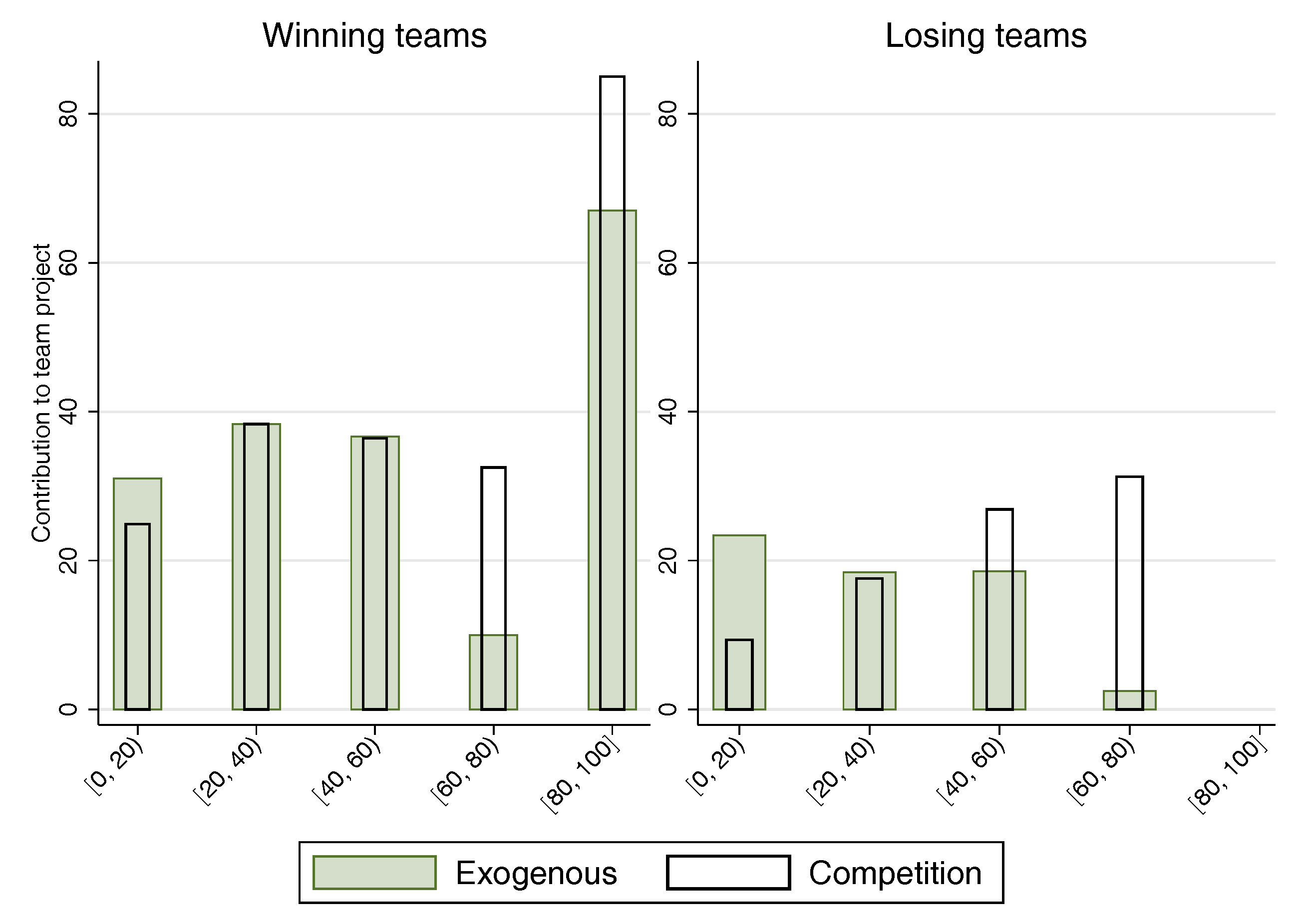
Figure 3 adds to the observation that there exists a somewhat heterogeneous relationship between treatments and winning and losing groups, respectively. The graph depicts the relationship between individual lottery tickets purchased (stage 1 contribution) and input into the team project. It appears that for both winning and losing teams in the competition treatment, it is the players who contributed more to the between group contest before, who also chip in for the team project subsequently. For the exogenous treatment this seems considerably less clear cut. This conjecture is confirmed by the results of a Spearman test, where for the competition treatment, both individuals from winning (Spearman test: N = 48, Spearman’s rho = 0.415, P = 0.003) and losing teams (Spearman test: N = 48, Spearman’s rho = 0.429, P = 0.002) display a significant positive correlation between stage 1 and stage 2 contributions. For the exogenous treatment, neither individuals from the winning (Spearman test: N = 48, Spearman’s rho = 0.100, P = 0.512) nor the losing teams (Spearman test: N = 48, Spearman’s rho = −0.186, P = 0.222) display a significant correlation in this regard.
Figure 4 depicts jittered scatter plots for each of the four situations, as outlined above. It captures the heterogeneous effect of first stage contribution on players’ willingness to cooperate in the team project. The solid line represents the fitted values determined by Tobit regression, with clustered standard error at the group level and boundaries at 0 and 100. For the losing teams, the treatment difference in the relationship between lottery tickets and contribution to the team project becomes apparent. While it is a sharply increasing function for the competition treatment, it has a negative slope in the exogenous treatment.
5.4. Regression to the Mean
In Section 1 we argue that participants who find themselves in the position of the group’s “workhorse”—by having purchased more lottery tickets than their teammates—could cut back on second stage contribution because of a feeling of entitlement of the sort “I brought us here, now you pay me off”. Figure 5 illustrates this regression to the mean effect in a jittered scatter plot with individual first stage contribution relative to the average of the other team members on the x-axis and the difference between individual first and second stage contribution on the y-axis. The solid line represents the fitted OLS regression with standard errors clustered at the group level. Indeed, participants who contribute more relative to their other group members in the first stage, tend to reduce their spending level in the second stage, which is indicated by the fitted line’s negative slope (OLS regression with clustered standard errors. N = 186, Coef. = −0.549, P = 0.000).
This result relates to our findings discussed above insofar as that the positive relationship between first and second stage contribution prevails from a general perspective. Yet overall spread between contributors and defectors gets weakened.
6. Discussion
In this article we present an experimental study in which we analyse how individuals react to heterogeneous sunk costs in a public good games setting. Specifically, we investigate two types of sunk costs: Deliberately accrued expenses and exogenously imposed deductions. We argue that although they are economically equivalent, players will not derive the same consequences.
Players in the competition treatment spend resources to influence the probability for getting their group sorted into a public good game with a higher MPCR. Players in the exogenous treatment, on the other hand, do not make this decision themselves. Instead there is a one-on-one matching with the contest from the competition treatment.
Standard Nash equilibrium under risk-neutrality and individualistic preferences would predict zero contribution to both stages of the experiment. By contrast, most players spend positive amounts in both games, dismissing Hypothesis 1. In Hypotheses 2 and 3, as well as Equation (1) we specify our hypothesis concerning the average contribution levels for the four different scenarios. While our data clearly indicates a higher contribution level for those groups that have been sorted to the higher MPCR game, results for the other two inequalities are considerably less clear cut. Only when controlling for outcome-specific level effects, we find some evidence that losing groups in the exogenous treatment spend more than their counterpart from the competition treatment. In our tests for Hypotheses 4 and 5 we examine the interrelation of first and second stage contribution. Our results corroborate Hypothesis 4 at the expense of its counter-hypotheses 5 and 6. The positive relationship between first and second stage contribution mainly prevails in the competition treatment, where it is utilised as costly signalling and sacrifice.
Furthermore, players in the competition treatment have a slightly higher tendency to refrain from contributing to the public good, when their team has lost. An equivalent higher contribution level for winning groups in the competition treatment, however, cannot be observed.
This means that players in the underlying game do not perceive a positive outcome of the between-group contest as signal for their group-mates’ willingness to cooperate, as compared to when they reach the high MPCR by exogenous sorting. At the same time, participants display a reduced willingness to cooperate with their teammates, when the group failed to attain the high MPCR game in the contest, as compared to the exogenous sorting.
Coming back to the aforementioned case of between company competition for a business deal, the implications derived from our results, vindicate a rather sceptical angle on a tendering of commercial covenants. If both candidates dispose of comparable productivity levels, the harm to the losing party is not met by an analogous positive burst of the winning party. From an overall social welfare perspective, devising a method of arbitration which avoids a between group contest would be favourable. To further test this policy advice, different ways of arbitration could be examined: Make both parties pay in equal amounts, or have the winner pay for it completely, among other conceivable sharing rules. The caveat of a subliminal latent contest might still apply in most settings, however.
7. Materials and Methods
7.1. Instructions
The instructions consisted of two parts. When entering the computer laboratory, participants found a printed copy of the first-part of instructions at their seat. They learned about the structure of the experiment, the exchange rate between points and pound sterling, as well as the SVO measure. The instructions were read aloud before participants started with the SVO slider task. After this, the second set of instructions was handed out, in which the main part of the experiment was explained. These instructions were read aloud as well. Paragraphs starting with a treatment name in square brackets were only given to participants of that particular treatment.
7.1.1. Instructions Part 1
Welcome and thank you for participating in this experiment. Please read these instructions carefully. If you have any questions, please raise your hand and one of the experimenters will come to your cubicle to answer your question. Talking or using mobile phones or any other electronic devices is strictly prohibited. Mobile phones and other electronic devices should be switched off. If you are found violating these rules, you will both forfeit any earnings from this experiment, and may be excluded from future experiments as well.
This is an experiment about decision making. The instructions are simple and if you follow them carefully you might earn a considerable amount of money which will be paid to you privately and in cash at the end of today’s session. The amount of money you earn depends on your decisions, on other participants’ decisions and on random events. You will never be asked to reveal your identity to anyone during the course of the experiment. Your name will never be associated with any of your decisions. To keep your decisions private, do not reveal your choices to any other participant.
During the experiment you will have the chance to earn points, which will be converted into cash at the end of today’s session, using an exchange rate of
1 point = 5 pence.
Thus, the more points you earn, the more cash you will receive at the end of the session.
This experiment consists of two parts. The following instructions explain Part 1. After finishing this part, you will receive further instructions for Part 2. None of your (or anyone else’s) decisions for one part are relevant for your (or anyone else’s) performance in the other part.
Part 1: In this task you will be randomly paired with another person in this room. You will make a series of decisions about allocating points between you and the other person.
Then one of you will be assigned the role of Sender and the other one the role of Receiver. If you are the Sender, ONE of your decisions will be picked randomly and implemented for both of you (i.e., you receive what you allocated to yourself and the other person receives what you allocated to her).
If you are assigned the role of Receiver, ONE decision of the other person will be picked randomly and implemented for both of you (i.e., you receive what the other person allocated to you and the other person receives what she allocated to herself).
All of your choices are completely confidential. You will learn your results of Part 1 after Part 2 has finished. Points earned in Part 1 and Part 2 will be added up to determine your total earnings.
7.1.2. Instructions Part 2
In Part 2, all participants are assigned to teams of three and your team will be matched with another team. None of you will learn the identities of own team members or other team members. Part 2 will consist of two stages:
[Competition treatment:] At the beginning of the first stage you will receive 200 points. Then you can use up to 100 of your points to buy lottery tickets for your team. Each lottery ticket costs 1 point. Any of your points not spent on lottery tickets will be accumulated in your private point balance. Likewise, each of your team members receives 200 points and can use up to 100 of these points to buy lottery tickets for your team. Similarly, each member of the other team will receive 200 points and can buy tickets for their team in exactly the same way.
[Exogenous treatment:] At the beginning of the first stage you will receive 200 points. Then the computer can use up to 100 of your points to buy lottery tickets for your team. Each lottery ticket costs 1 point. Any of your points not spent on lottery tickets will be accumulated in your private point balance. Likewise, each of your team members receives 200 points and the computer can use up to 100 of these points to buy lottery tickets for your team. Similarly, each member of the other team will receive 200 points and the computer can buy tickets for their team in exactly the same way.
Next, a lottery will determine whether your team, or the team you are matched with wins. One of the tickets is randomly selected to be the winning ticket. Each ticket has the same chance. Hence, the more tickets your team has, the higher is your team’s chance of winning.
Examples: If your team and the other team have the same amount of tickets then each team is equally likely to win. If your team has three times as many tickets as the other team, then your team is three times as likely to win as the other team. If only one of the teams has tickets, then this team wins with certainty. If neither your team nor the other team has any tickets, then one of the teams will be randomly selected as the winner with each team equally likely to be selected.
After the winning team is determined you will reach the second stage. You will be able to see the following information: Individual tickets for each of your team mates, other team’s tickets and your winning probability. The second stage differs between the winning and the losing team in one way, which will be underlined below.
In the second stage you can invest up to 100 points of your endowment in a team project. Any point you do not invest and keep to yourself will be accumulated in your private point balance. Each point invested in the team project yields 0.8 points for you and every member of your team, if your team has won in the first stage. Similarly, each point invested in the team project yields 0.4 points for you and every member of your team if your team has lost in the first stage. Likewise, your team members can invest in the team project in the same way.
A summary of how your Part 2 earnings will be determined is provided on the next page.
This part starts with a trial period in which you will be asked to answer some questions in order to check your understanding and to give you the opportunity to get acquainted with the setup. Points earned in this trial period will not be paid off.
Summary:
Your earnings for this part are determined as follows:
| Winning team: | |
| Your Endowment | |
| − | Your tickets (between 0 and 100) |
| − | Your contribution to the team project (between 0 and 100) |
| + | your team’s total contribution to the team project |
| = | Your earnings |
| Losing team: | |
| Your Endowment | |
| − | Your tickets (between 0 and 100) |
| − | Your contribution to the team project (between 0 and 100) |
| + | your team’s total contribution to the team project |
| = | Your earnings |
Supplementary Materials
The supplementary materials are available at https://www.mdpi.com/2073-4336/9/3/41/s1.
Author Contributions
Conceptualization, F.H. and M.S.; Methodology, F.H. and M.S.; Software, F.H.; Validation, F.H. and M.S.; Formal Analysis, F.H. and M.S.; Investigation, F.H. and Valeria Burdea; Resources, F.H. and M.S.; Data Curation, F.H.; Writing—Original Draft Preparation, F.H.; Writing—Review & Editing, F.H. and M.S.; Visualization, F.H.; Supervision, M.S.; Project Administration, F.H.; Funding Acquisition, F.H. and M.S.
Funding
Financial support from the Gesellschaft für experimentelle Wirtschaftsforschung e.V. (GfeW) through the “Heinz Sauermann-Förderpreis zur experimentellen Wirtschaftsforschung” grant is gratefully acknowledged.
Acknowledgments
We would like to thank Valeria Burdea for invaluable help in the realisation of the experiment.
Conflicts of Interest
The authors declare no conflict of interest. The founding sponsors had no role in the design of the study; in the collection, analyses, or interpretation of data; in the writing of the manuscript, and in the decision to publish the results.
Appendix A. Social Value Orientation-Measure
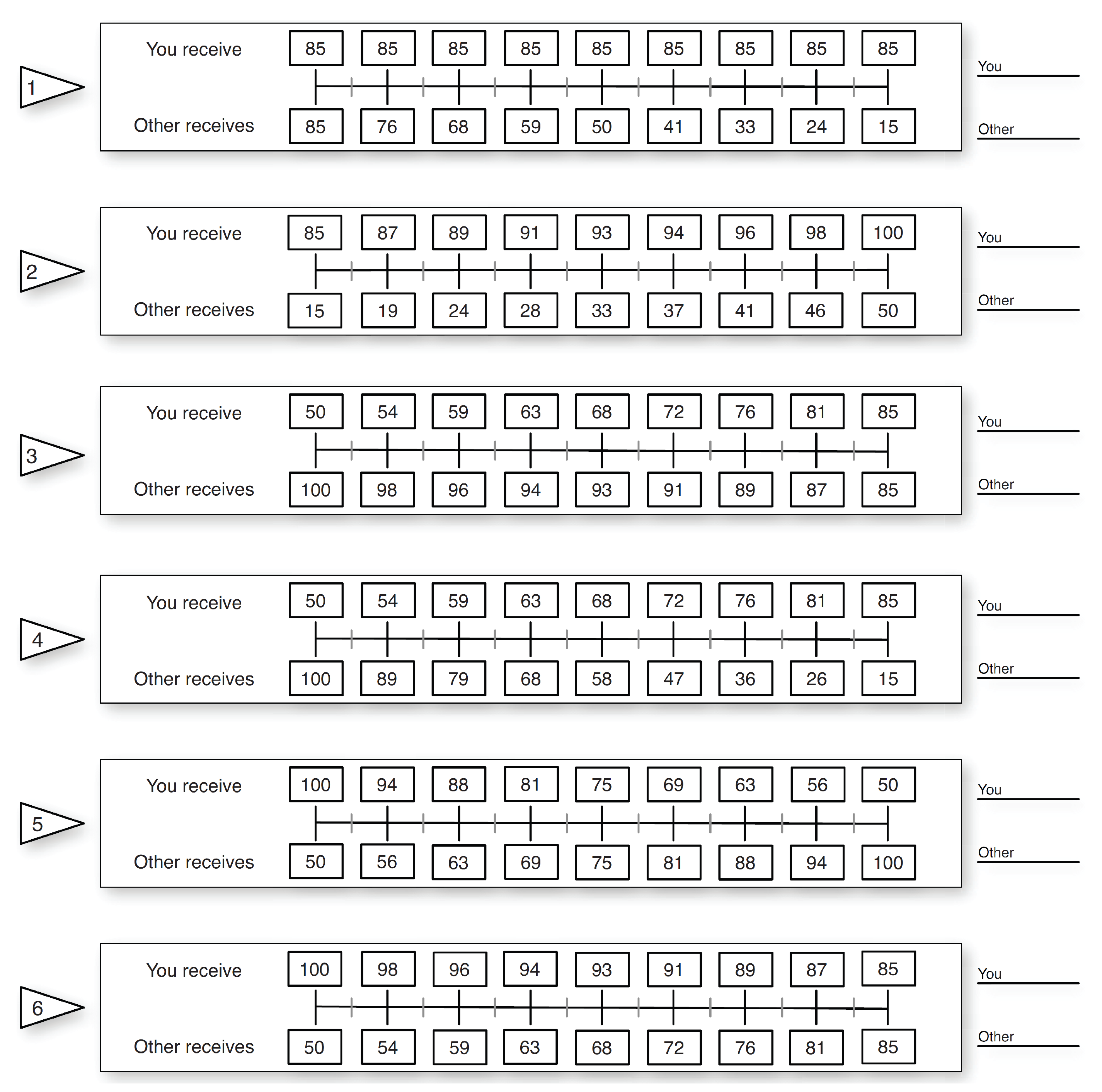
Prior to the main part of the experiment, we take a measurement of individual social preferences, using the SVO slider measure by [30].24 Participants set six sliders to determine mutual sharing of an amount of tokens, as represented in Figure A1. This was incentivised in the following way: After all participants cast their decisions, pairs of two were randomly created with one being the Sender and the other participant being the Receiver. One of the Sender’s decisions was implemented on both at random, where the Sender gets what she allocated to herself and the Receiver gets what the Sender allocated to her. Participants only got to know, which allocation was chosen to be paid out, after the main part of the experiment.
This technique was a simplification and adjustment of the circle test employed by [57,58]. It has demonstrated reliable psychometric properties, yields scores for individuals at the ratio level and is quick and easy to implement cf. [59].
Figure A1.
Slider questions to measure Social Value Orientation as seen by participants.

Appendix B. Risk Neutral Equilibrium
- Second stage
- Players individually maximise their profit by setting own contribution :with . As and , there exists a corner solution .
- First stage
- Under common knowledge of rationality, players know that and maximisewith being the expected earnings from stage 2. Again, a corner solution exists with .
Appendix C. Contest Expenditures—The Role of Beliefs
About 10% of first stage contributions fall in an area which is not rationalisable (i.e., contributions larger than 65), even holding the most optimistic beliefs about the second stage (i.e., all other players contribute fully), while at the same time holding very pessimistic beliefs about groupmates’ behaviour in the first stage (i.e., no other groupmate buys lottery tickets). When holding the same beliefs on second stage contributions, while assuming symmetry in first stage spending levels, some 46% fall in the category of non-rationalisability (contributions larger than ).
- Second stage
- Player i’s payoff depends positively on her teammates’ input towards the team project , as in:Hence, player i’s most optimistic belief for the second stage would involve full contribution by all other group members, i.e., , which would amount to an account of and expected second stage earnings of for a winning group.
- First stage
- Most pessimistic beliefs about teammates’ contest spending behaviour are characterised as . If all teammates do not buy lottery tickets () and expected second stage payoff , player i maximises Equation (A2) at .Consider as alternative belief on first stage behaviour, that all teammates contribute symmetrically, i.e., . For this set of beliefs, Equation (A2) maximises at .
Appendix D. Additional Regressions
Table A1 shows results for OLS regressions of determinants of individual contribution to the between group contest akin to Table 1. Results stay qualitatively similar and the interpretation corresponds with Section 5.1.

Table A1.
Determinants of stage 1 contribution—OLS Regression.
| Variables | (7) | (8) |
|---|---|---|
| First Stage Contribute | ||
| Social value orientation (SVO) | 0.529 ** | 0.395 * |
| (0.22) | (0.22) | |
| Risk parameter | 2.708 | |
| (2.03) | ||
| Female | 15.299 ** | |
| (6.55) | ||
| Age | 3.567 ** | |
| (1.49) | ||
| Number of siblings | −1.632 | |
| (2.76) | ||
| Smoking | 3.882 | |
| (12.64) | ||
| Politics important | −3.164 | |
| (3.65) | ||
| Trust in others | 13.727 ** | |
| (5.96) | ||
| Income Equality | −3.067 * | |
| (1.78) | ||
| Hard work | −1.119 | |
| (1.69) | ||
| Constant | 19.614 *** | −73.035 * |
| (4.62) | (36.93) | |
| N | 96 | 93 |
| R-squared | 0.060 | 0.435 |
* p < 0.10, ** p< 0.05, *** p< 0.01; Standard errors in parentheses. Study major dummies not listed.
Complementing Table 3, we present results for OLS regressions with robust standard errors for intra-group correlation in Table A2. We analyse the relationship between contribution to the team project and first stage contribution, including outcome dummies, interaction effects and controls. Results stay fairly comparable overall, between the two regression methods.
As alternative, we analyse each of the four outcomes separately. For this, we regress contribution to the team project on first stage contribution and a few controls using a Tobit model with robust standard errors for intragroup correlation and limits at 0 and 100.25 Consider Table A3a,b with losing/winning groups of the exogenous and losing/winning groups of the competition treatment, each with and without control variables.
Table A2.
Determinants of stage 2 contribution—OLS Regression.
| Variables | (9) | (10) | (11) | (12) |
|---|---|---|---|---|
| Second Stage Contribute | ||||
| First stage | 0.241 *** | 0.210 ** | 0.269 * | 0.336 * |
| Contribute | (0.09) | (0.10) | (0.14) | (0.19) |
| Group Contribute | 0.108 * | 0.093 | 0.149 ** | 0.117 |
| Minus Self | (0.06) | (0.07) | (0.06) | (0.08) |
| Social value | 0.435 ** | 0.327 * | 0.355 * | 0.284 |
| orientation (SVO) | (0.18) | (0.19) | (0.19) | (0.19) |
| Exogenous lose | 2.557 | 5.381 | 17.171 ** | 18.633 * |
| (5.26) | (6.09) | (7.57) | (10.52) | |
| Exogenous win | 12.196 * | 12.697 * | 12.421 * | 16.964 * |
| (6.58) | (6.40) | (6.68) | (8.50) | |
| Competition win | 15.012 *** | 13.994 ** | 5.377 | 9.693 |
| (5.37) | (6.73) | (8.31) | (10.72) | |
| Exogenous lose | −0.635 *** | −0.577 * | ||
| × First stage Contr. | (0.21) | (0.30) | ||
| Exogenous win | −0.039 | −0.181 | ||
| × First stage Contr. | (0.18) | (0.24) | ||
| Competition win | 0.249 | 0.072 | ||
| × First stage Contr. | (0.21) | (0.27) | ||
| Constant | −1.255 | −39.688 | −2.461 | −39.307 |
| (4.85) | (32.75) | (5.41) | (34.09) | |
| Controls | No | Yes | No | Yes |
| N | 186 | 181 | 186 | 181 |
| R-squared | 0.166 | 0.310 | 0.221 | 0.336 |
* p < 0.10, ** p< 0.05, *** p< 0.01; Robust standard errors in parentheses, clustered at group level. Study major dummies not listed.
Table A3.
Tobit models with limits at 0 and 100.
| (a) Exogenous Treatment. | ||||
| Variables | Contribution to the Team Project | |||
| (13) | (14) | (15) | (16) | |
| Exogenous Lose | Exogenous Win | |||
| First stage | −0.896 ** | −0.559 | 0.205 | 0.504 * |
| Contribute | (0.38) | (0.36) | (0.33) | (0.25) |
| Group Contribute | 0.142 | 0.076 | 0.570 *** | 0.619 *** |
| Minus Self | (0.24) | (0.20) | (0.18) | (0.14) |
| Social value | 0.062 | 0.025 | −0.033 | 0.335 |
| orientation (SVO) | (0.45) | (0.32) | (0.51) | (0.62) |
| Constant | −35.603 | 14.801 | −245.801 ** | −41.283 ** |
| (70.81) | (14.87) | (102.83) | (20.20) | |
| Controls | Yes | No | Yes | No |
| N | 43 | 45 | 45 | 45 |
| Pseudo R-squared | 0.138 | 0.008 | 0.143 | 0.035 |
| (b) Competition Treatment. | ||||
| Variables | Contribution to the Team Project | |||
| (17) | (18) | (19) | (20) | |
| Competition Lose | Competition Win | |||
| First stage | −0.095 | 0.817 ** | 0.080 | 0.664 ** |
| Contribute | (0.26) | (0.35) | (0.26) | (0.31) |
| Group Contribute | 0.509 *** | 0.572 *** | 0.003 | −0.066 |
| Minus Self | (0.18) | (0.19) | (0.20) | (0.23) |
| Social value | 1.852 ** | 1.646 ** | 1.020 ** | 1.671 * |
| orientation (SVO) | (0.71) | (0.73) | (0.37) | (0.91) |
| Constant | 58.374 | −85.612 *** | −333.308 *** | −15.653 |
| (79.29) | (23.42) | (82.57) | (25.38) | |
| Controls | Yes | No | Yes | No |
| N | 46 | 48 | 47 | 48 |
| Pseudo R-squared | 0.206 | 0.074 | 0.203 | 0.056 |
* p < 0.10, ** p< 0.05, *** p< 0.01; Robust standard errors in parentheses, clustered at group level. Study major dummies not listed.
For the competition treatment there mostly exists a clear positive relationship between contribution to the lottery game and to the team project. This means that relatively poorer individuals spend more for the team project. This is not the case, however, for the exogenous treatment: Regression (13) displays a significant negative coefficient, while Regression (16) has a significantly positive relationship. The group contribution level plays a positive role as well in some regressions.
Social value orientation (SVO) only plays a role in the competition treatment in all regressions (17)–(20), where it is positive. This relationship does not exist, though, for the exogenous treatment, where the explanatory power of the SVO measure is not significantly different from zero.
Table A4.
Tobit model with limits at 0 and 100 testing if first stage contribution has a significant effect on second stage contribution.
Table A4.
Tobit model with limits at 0 and 100 testing if first stage contribution has a significant effect on second stage contribution.
| Variables | Second stage Contribute | |||
|---|---|---|---|---|
| (5.1) | (6.1) | (5.2) | (6.2) | |
| Exogenous lose | Exogenous win | |||
| First stage | -0.512 | -0.776** | 0.345 | -0.038 |
| Contribute | (0.32) | (0.32) | (0.24) | (0.36) |
| Social value | -0.018 | 0.116 | 0.141 | -0.197 |
| orientation (SVO) | (0.34) | (0.43) | (0.75) | (0.49) |
| Constant | 18.011 | -17.204 | 10.284 | -213.785* |
| (12.96) | (63.02) | (18.44) | (106.81) | |
| Controls | No | Yes | No | Yes |
| N | 45 | 43 | 45 | 45 |
| Pseudo R-squared | 0.008 | 0.137 | 0.005 | 0.117 |
* p < 0.10, ** p< 0.05; Robust standard errors in parentheses, clustered at group level. Study major dummies not listed.
Appendix E. Control Variables
Table A5 corresponds to Regressions (4) and (6) of Table 3 and displays the control variables, which were generated by a post-experiment questionnaire, in more detail. We do not have well-established hypotheses for each of these control variables, for why we present this section in an explorative character. In Table A6, which corresponds to Regressions (13), (15), (17) and (19) of Table A3a,b, we investigate on heterogeneities of these control variables between outcomes in the experiment.26
The risk parameter has explanatory power (all positive) only for some of the regressions in this section. It was generated by a self-reported risk tolerance indication on a scale from one to seven. As players invest resources without knowing the contribution level of other teammates, contributing involves a certain degree of risk taking. Accordingly, it seems intuitively plausible that individuals displaying a higher level of risk tolerance would also contribute more to the team project.
While being an overall noisy parameter, female seems to deliver some evidence that female participants follow a more cooperative strategy towards the public good. Unlike our results for gender effects in first stage contribution, this positive relationship seems in line with established literature e.g., [60].27
Table A5.
Determinants of stage 2 contribution. Tobit model with limits at 0 and 100—Control Variables.
Table A5.
Determinants of stage 2 contribution. Tobit model with limits at 0 and 100—Control Variables.
| Variables | (4) | (6) |
|---|---|---|
| Second Stage Contribute | ||
| First stage | 0.360 ** | 0.912 ** |
| Contribute | (0.17) | (0.37) |
| Group Contribute | 0.223 * | 0.262 ** |
| Minus Self | (0.12) | (0.12) |
| Social value | 0.809 ** | 0.721 ** |
| orientation (SVO) | (0.34) | (0.34) |
| Exogenous lose | 16.488 | 49.942 ** |
| (11.51) | (19.30) | |
| Exogenous win | 25.530 ** | 44.400 ** |
| (12.02) | (17.82) | |
| Competition win | 28.767 ** | 32.699 |
| (12.50) | (20.46) | |
| Risk parameter | 7.270 * | 6.264 |
| (3.69) | (3.94) | |
| Female | 10.767 | 8.824 |
| (10.13) | (9.35) | |
| Age | 3.484 * | 2.890 |
| (1.84) | (1.84) | |
| Number of siblings | 4.185 | 4.356 |
| (3.84) | (3.87) | |
| Smoking | −12.913 | −12.770 |
| (20.72) | (21.75) | |
| Politics important | −14.725 ** | −14.478 ** |
| (6.12) | (6.19) | |
| Trust in others | 11.438 | 7.464 |
| (7.79) | (7.63) | |
| Income Equality | 2.121 | 2.914 |
| (2.78) | (2.91) | |
| Hard work | −5.231 ** | −4.427 * |
| (2.47) | (2.50) | |
| Exogenous lose | −1.419 ** | |
| × First stage Contr. | (0.56) | |
| Exogenous win | −0.720 | |
| × First stage Contr. | (0.44) | |
| Competition win | −0.282 | |
| × First stage Contr. | (0.50) | |
| Constant | −127.493 ** | −130.816 ** |
| (50.81) | (53.69) | |
| N | 181 | 181 |
| Pseudo R-squared | 0.067 | 0.073 |
* p < 0.10, ** p< 0.05; Robust standard errors in parentheses, clustered at group level. Study major dummies not listed.
A factor that predominantly plays a role in the competition treatment is the age of participants. Interestingly, age seems to accentuate the difference between winning and losing groups along the lines of Hypothesis 1. By contrast, number of siblings slightly works in the opposite effect. Experimental results from a trust game in Glaeser et al. [62] suggest that individuals with siblings are a lot more trustworthy than only child individuals: the latter only returned about half as much money to the senders as the former. In our study, this effect only persists in losing groups with a lower structural contribution level. Therefore, number of siblings could represent a regression to the mean effect that attenuates “extreme” levels of contribution.
Table A6.
Effect of first stage contribution and dummies on cooperation level in the team project.
| Variables | Contribution to the Team Project | |||
|---|---|---|---|---|
| (13) | (15) | (17) | (19) | |
| Exogenous Lose | Exogenous Win | Competition Lose | Competition Win | |
| First stage | −0.896 ** | 0.205 | −0.095 | 0.080 |
| Contribute | (0.38) | (0.33) | (0.26) | (0.26) |
| Group Contribute | 0.142 | 0.570 *** | 0.509 *** | 0.003 |
| Minus Self | (0.24) | (0.18) | (0.18) | (0.20) |
| Social value | 0.062 | −0.033 | 1.852 ** | 1.020 ** |
| orientation (SVO) | (0.45) | (0.51) | (0.71) | (0.37) |
| Risk parameter | −2.719 | 15.760 * | −5.537 | 22.633 *** |
| (6.71) | (7.66) | (5.28) | (6.85) | |
| Female | 24.237 ** | 43.473 | 16.922 | 37.388 * |
| (11.42) | (25.80) | (15.72) | (19.14) | |
| Age | 2.839 | 1.104 | -2.599 | 12.741 *** |
| (2.58) | (2.24) | (3.64) | (2.79) | |
| Number of siblings | 9.572 | -3.455 | 21.426 *** | −11.312 * |
| (7.53) | (5.82) | (7.34) | (6.59) | |
| Smoking | −55.281 ** | 39.069 | -15.025 | −148.254 *** |
| (20.34) | (57.84) | (32.35) | (45.91) | |
| Politics important | −18.907 * | −8.347 | 1.375 | −10.476 |
| (10.23) | (11.49) | (7.77) | (7.65) | |
| Trust in others | 2.902 | −13.040 | 23.770 *** | 27.203 * |
| (12.70) | (17.80) | (6.93) | (15.56) | |
| Income Equality | 10.225 *** | 18.709 *** | −7.284 * | −19.230 *** |
| (3.37) | (5.10) | (3.68) | (6.72) | |
| Hard work | −7.560 | 9.919 | −7.221 ** | −9.436 ** |
| (4.70) | (6.21) | (3.07) | (4.19) | |
| Constant | -35.603 | −245.801 ** | 58.374 | −333.308 *** |
| (70.81) | (102.83) | (79.29) | (82.57) | |
| N | 43 | 45 | 46 | 47 |
| Pseudo R-squared | 0.138 | 0.143 | 0.206 | 0.203 |
* p < 0.10, ** p< 0.05, *** p< 0.01; Robust standard errors in parentheses, clustered at group level. Study major dummies not listed.
In the questionnaire we asked participants whether they smoke or not and if they do so regularly or only sometimes. We include this parameter as proxy for short-sightedness of utility horizons cp. [63]. Indeed, participants with a higher self-reported level of tobacco consumption, seem to contribute less to the team project. This effect is only reflected in Regressions (13) and (19), though. In consonance with the line of reasoning in Slovic [63], we construe that (frequent) smokers exhibit a shorter time horizon for their decisions. Accordingly, they pick the bird in the hand—keep the 100 tokens to themselves—over the two in the bush—potential gains from the group project.
Also for Politics important we can identify some evidence that this factor negatively influences second stage spending in Regressions (4), (6) and (13). Politics important has been generated using a scale from 1–4, where participants were asked how important they find politics in their life. If interpreting this factor as akin to individual Public Service Motivation (PSM), its negative effect on players’ level of cooperativeness seems rather unintuitive. Esteve et al. [64], for example show that individuals with higher levels of PSM exert more effort for their communities and societies.
In line with arguments from Section 5.1, we would expect participants with a higher Trust in others28 to be more cooperative in the team project. Only two of the regressions confirm this hypothesis, while this variable stays insignificant in the other regressions.
For the factor income equality, individuals stated their proximity to which of the two following statements they feel closer on a scale from one to seven: “We need larger income differences as incentives for individual effort.”—“Incomes should be made more equal.” Accordingly, this factor aims at capturing individual preferences for either a steep or flat income curve. Results for income equality identify opposite effects for the two treatments. While there seems to be a positive relationship in the exogenous treatment, the parameter turns negative for regressions using players from the competition treatment.
The last parameter, hard work intends to pick up a certain dog-eat-dog mentality as in whether participants believe that everyone is the architect of ones own fortune or if success is a matter of luck. On a scale from one to seven, participants express their proximity to one of the two statements: “Hard work doesn’t generally bring success; it’s more a matter of luck and connections.”—“In the long run, hard work usually brings a better life.” Those participants who rather believe that hard work pays off—“man forges his own destiny”—are less willing to contribute to the group account in the team project phase of the game. We find support for this hypothesis in most of the underlying regressions.
References
- Tullock, G. Efficient Rent Seeking. In Toward a Theory of the Rent-Seeking Society; Buchanan, J., Tollison, R., Tullock, G., Eds.; Texas A & M University Press: College Station, TX, USA, 1980; pp. 97–112. [Google Scholar]
- Katz, E.; Nitzan, S.; Rosenberg, J. Rent-seeking for pure public goods. Public Choice 1990, 65, 49–60. [Google Scholar] [CrossRef]
- Baye, M.R.; Hoppe, H.C. The strategic equivalence of rent-seeking, innovation, and patent-race games. Games Econ. Behav. 2003, 44, 217–226. [Google Scholar] [CrossRef] [Green Version]
- Bornstein, G.; Gneezy, U. Price Competition Between Teams. Exp. Econ. 2002, 5, 29–38. [Google Scholar] [CrossRef]
- Stub, S.T. Boeing, Airbus in Dogfight Over El Al. Wall Street J. 2012. Available online: http://www.wsj.com/articles/SB10001424052702303665904577452612947594688 (accessed on 25 June 2018).
- Fouzder, M. Legal aid tenders: ‘hundreds’ of firms will go under. Law Soc. Gaz. 2015. Available online: https://www.lawgazette.co.uk/law/legal-aid-tenders-hundreds-of-firms-will-go-under/5047915.fullarticle (accessed on 25 June 2018).
- Arkes, H.R.; Blumer, C. The psychology of sunk cost. Organ. Behav. Hum. Decis. Process. 1985, 35, 124–140. [Google Scholar] [CrossRef]
- Whyte, G. Escalating Commitment in Individual and Group Decision Making: A Prospect Theory Approach. Organ. Behav. Hum. Decis. Process. 1993, 54, 430–455. [Google Scholar] [CrossRef]
- Fehr, E.; Schmidt, K.M. A Theory of Fairness, Competition, and Cooperation. Q. J. Econ. 1999, 114, 817–868. [Google Scholar] [CrossRef] [Green Version]
- Savikhin, A.C.; Sheremeta, R.M. Simultaneous decision-making in competitive and cooperative environments. Econ. Inq. 2013, 51, 1311–1323. [Google Scholar] [CrossRef]
- Godoy, S.; Morales, A.J.; Rodero, J. Competition lessens competition: An experimental investigation of simultaneous participation in a public good game and a lottery contest game with shared endowment. Econ. Lett. 2013, 120, 419–423. [Google Scholar] [CrossRef]
- Dechenaux, E.; Kovenock, D.; Sheremeta, R. A survey of experimental research on contests, all-pay auctions and tournaments. Exp. Econ. 2015, 18, 609–669. [Google Scholar] [CrossRef]
- Konrad, K.A. Strategy and Dynamics in Contests; Oxford University Press: Oxford, UK, 2009. [Google Scholar]
- Abbink, K.; Brandts, J.; Herrmann, B.; Orzen, H. Intergroup Conflict and Intra-Group Punishment in an Experimental Contest Game. Am. Econ. Rev. 2010, 100, 420–447. [Google Scholar] [CrossRef] [Green Version]
- Gunnthorsdottir, A.; Rapoport, A. Embedding social dilemmas in intergroup competition reduces free-riding. Organ. Behav. Hum. Decis. Process. 2006, 101, 184–199. [Google Scholar] [CrossRef]
- Bornstein, G.; Kugler, T.; Budescu, D.V.; Selten, R. Repeated price competition between individuals and between teams. J. Econ. Behav. Organ. 2008, 66, 808–821. [Google Scholar] [CrossRef]
- Morgan, J.; Orzen, H.; Sefton, M.; Sisak, D. Strategic and Natural Risk in Entrepreneurship: An Experimental Study. J. Econ. Manag. Strategy 2016, 25, 420–454. [Google Scholar] [CrossRef]
- Huyck, J.B.V.; Battalio, R.C.; Beil, R.O. Asset Markets as an Equilibrium Selection Mechanism: Coordination Failure, Game Form Auctions, and Tacit Communication. Games Econ. Behav. 1993, 5, 485–504. [Google Scholar] [CrossRef]
- Cooper, D.J.; Ioannou, C.A.; Qi, S. Coordination with Endogenous Contracts: Incentives, Selection, and Strategic Anticipation. Available online: http://myweb.fsu.edu/djcooper/research/selectionandcoordination.pdf (accessed on 25 June 2018).
- Frank, R.H. If Homo Economicus Could Choose His Own Utility Function, Would He Want One with a Conscience? Am. Econ. Rev. 1987, 77, 593–604. [Google Scholar]
- Amann, E.; Yang, C.L. Sophistication and the persistence of cooperation. J. Econ. Behav. Organ. 1998, 37, 91–105. [Google Scholar] [CrossRef]
- Orbell, J.; Dawes, R.M. A “Cognitive Miser” Theory of Cooperators Advantage. Am. Polit. Sci. Rev. 1991, 85, 515–528. [Google Scholar] [CrossRef]
- Orbell, J.M.; Dawes, R.M. Social Welfare, Cooperators’ Advantage, and the Option of Not Playing the Game. Am. Sociol. Rev. 1993, 58, 787–800. [Google Scholar] [CrossRef]
- Nosenzo, D.; Tufano, F. The Effect of Voluntary Participation on Cooperation. J. Econ. Behav. Organ. 2017, 142, 307–319. [Google Scholar] [CrossRef]
- Garland, H. Throwing good money after bad: The effect of sunk costs on the decision to esculate commitment to an ongoing project. J. Appl. Psychol. 1990, 75, 728. [Google Scholar] [CrossRef]
- Kahneman, D.; Tversky, A. Prospect Theory: An Analysis of Decision under Risk. Econometrica 1979, 47, 263–292. [Google Scholar] [CrossRef]
- Staw, B.M. The Escalation of Commitment to a Course of Action. Acad. Manag. Rev. 1981, 6, 577–587. [Google Scholar] [CrossRef]
- Friedman, D.; Pommerenke, K.; Lukose, R.; Milam, G.; Huberman, B. Searching for the sunk cost fallacy. Exp. Econ. 2007, 10, 79–104. [Google Scholar] [CrossRef] [Green Version]
- Offerman, T.; Potters, J. Does auctioning of entry licences induce collusion? An experimental study. Rev. Econ. Stud. 2006, 73, 769–791. [Google Scholar] [CrossRef]
- Murphy, R.O.; Ackermann, K.A.; Handgraaf, M.J. Measuring social value orientation. Judgm. Decis. Mak. 2011, 6, 771–781. [Google Scholar] [CrossRef]
- Balliet, D.; Parks, C.; Joireman, J. Social Value Orientation and Cooperation in Social Dilemmas: A Meta-Analysis. Group Process. Intergroup Relat. 2009, 12, 533–547. [Google Scholar] [CrossRef]
- Greiner, B. The online recruitment system ORSEE 2.0. In A Guide for the Organization of Experiments in Economics; University of Cologne: Cologne, Germany, 2004. [Google Scholar]
- Fischbacher, U. z-Tree: Zurich toolbox for ready-made economic experiments. Exp. Econ. 2007, 10, 171–178. [Google Scholar] [CrossRef] [Green Version]
- Glöckner, A.; Irlenbusch, B.; Kube, S.; Nicklisch, A.; Normann, H.T. Leading with (out) sacrifice? A public-goods experiment with a privileged player. Econ. Inq. 2011, 49, 591–597. [Google Scholar] [CrossRef]
- Gunnthorsdottir, A.; Houser, D.; McCabe, K. Disposition, history and contributions in public goods experiments. J. Econ. Behav. Organ. 2007, 62, 304–315. [Google Scholar] [CrossRef] [Green Version]
- Isaac, R.M.; Walker, J.M. Group Size Effects in Public Goods Provision: The Voluntary Contributions Mechanism. Q. J. Econ. 1988, 103, 179–199. [Google Scholar] [CrossRef]
- Bednar, J.; Chen, Y.; Liu, T.X.; Page, S. Behavioral spillovers and cognitive load in multiple games: An experimental study. Games Econ. Behav. 2012, 74, 12–31. [Google Scholar] [CrossRef] [Green Version]
- Cason, T.N.; Savikhin, A.C.; Sheremeta, R.M. Behavioral spillovers in coordination games. Eur. Econ. Rev. 2012, 56, 233–245. [Google Scholar] [CrossRef] [Green Version]
- Capraro, V. A Model of Human Cooperation in Social Dilemmas. PLoS ONE 2013, 8, 1–6. [Google Scholar] [CrossRef] [PubMed]
- Reuben, E.; Riedl, A. Enforcement of contribution norms in public good games with heterogeneous populations. Games Econ. Behav. 2013, 77, 122–137. [Google Scholar] [CrossRef] [Green Version]
- Heap, S.P.H.; Ramalingam, A.; Stoddard, B.V. Endowment inequality in public goods games: A re-examination. Econ. Lett. 2016, 146, 4–7. [Google Scholar] [CrossRef] [Green Version]
- Anderson, L.R.; Mellor, J.M.; Milyo, J. Inequality and public good provision: An experimental analysis. J. Socio Econ. 2008, 37, 1010–1028. [Google Scholar] [CrossRef]
- Buckley, E.; Croson, R. Income and wealth heterogeneity in the voluntary provision of linear public goods. J. Public Econ. 2006, 90, 935–955. [Google Scholar] [CrossRef]
- Bolton, G.E.; Ockenfels, A. ERC: A Theory of Equity, Reciprocity, and Competition. Am. Econ. Rev. 2000, 90, 166–193. [Google Scholar] [CrossRef] [Green Version]
- Wilcoxon, F. Individual Comparisons by Ranking Methods. Biom. Bull. 1945, 1, 80–83. [Google Scholar] [CrossRef]
- Mann, H.B.; Whitney, D.R. On a Test of Whether one of Two Random Variables is Stochastically Larger than the Other. Ann. Math. Stat. 1947, 18, 50–60. [Google Scholar] [CrossRef]
- Spearman, C. The proof and measurement of association between two things. Am. J. Psychol. 1904, 15, 72–101. [Google Scholar] [CrossRef]
- Conover, W. Practical Nonparametric Statistics, 3rd ed.; Wiley: New York, NY, USA, 1999. [Google Scholar]
- Angrist, J.D.; Pischke, J.S. Mostly Harmless Econometrics an Empiricist’s Companion; Princeton University Press: Princeton, NJ, USA, 2009. [Google Scholar]
- Rogers, W. Regression standard errors in clustered samples. Stata Tech. Bull. 1994, 3, 19–23. [Google Scholar]
- McDonald, M.M.; Navarrete, C.D.; Van Vugt, M. Evolution and the psychology of intergroup conflict: The male warrior hypothesis. Philos. Trans. R. Soc. Lond. B Biol. Sci. 2012, 367, 670–679. [Google Scholar] [CrossRef] [PubMed]
- Vugt, M.V.; Cremer, D.D.; Janssen, D.P. Gender Differences in Cooperation and Competition: The Male-Warrior Hypothesis. Psychol. Sci. 2007, 18, 19–23. [Google Scholar] [CrossRef] [PubMed]
- Babcock, L.; Recalde, M.P.; Vesterlund, L.; Weingart, L. Gender Differences in Accepting and Receiving Requests for Tasks with Low Promotability. Am. Econ. Rev. 2017, 107, 714–747. [Google Scholar] [CrossRef] [Green Version]
- Martin, J.J.; Ecklund, R.C.; Smith, A.L. The relationships among competitiveness, age and ability in distance runners. J. Sport Behav. 1994, 17, 258. [Google Scholar]
- Inglehart, R.; Archivo de Estudios Sociales. World Values Surveys and European Values Surveys, 1981–1984, 1990–1993, and 1995–1997; ICPSR: Ann Arbor, MI, USA, 2000. [Google Scholar]
- Crosetto, P.; Weisel, O.; Winter, F. A flexible z-Tree implementation of the Social Value Orientation Slider Measure (Murphy et al. 2011): Manual; Technical Report, Jena Economic Research Papers; Friedrich-Schiller-University: Jena, Germany, 2012. [Google Scholar]
- Brandts, J.; Riedl, A.; van Winden, F. Competitive rivalry, social disposition, and subjective well-being: An experiment. J. Public Econ. 2009, 93, 1158–1167. [Google Scholar] [CrossRef] [Green Version]
- Sonnemans, J.; van Dijk, F.; van Winden, F. On the dynamics of social ties structures in groups. J. Econ. Psychol. 2006, 27, 187–204. [Google Scholar] [CrossRef] [Green Version]
- Murphy, R.O.; Ackermann, K.A. Social Value Orientation: Theoretical and Measurement Issues in the Study of Social Preferences. Pers. Soc. Psychol. Rev. 2014, 18, 13–41. [Google Scholar] [CrossRef] [PubMed]
- Stockard, J.; van de Kragt, A.J.C.; Dodge, P.J. Gender Roles and Behavior in Social Dilemmas: Are There Sex Differences in Cooperation and in Its Justification? Soc. Psychol. Q. 1988, 51, 154–163. [Google Scholar] [CrossRef]
- Sell, J.; Kuipers, K.J. A Structural Social Psychological View of Gender Differences in Cooperation. Sex Roles 2009, 61, 317–324. [Google Scholar] [CrossRef]
- Glaeser, E.L.; Laibson, D.I.; Scheinkman, J.A.; Soutter, C.L. Measuring Trust. Q. J. Econ. 2000, 115, 811–846. [Google Scholar] [CrossRef]
- Slovic, P. Smoking: Risk, Perception, and Policy; Sage Publications: Thousand Oaks, CA, USA, 2001. [Google Scholar]
- Esteve, M.; Urbig, D.; van Witteloostuijn, A.; Boyne, G. Prosocial Behavior and Public Service Motivation. Public Adm. Rev. 2016, 76, 177–187. [Google Scholar] [CrossRef]
| 1. | |
| 2. | Public procurement procedures for legal aid providers in the UK illustrate a related application: Legal firms enter a tendering process for duty provider contracts. While this represents an attractive business for legal enterprises, there is a considerable amount of firms operating without duty work. In 2015, around 200 firms won no contract and currently operate without duty work [6] in press. |
| 3. | |
| 4. | Details are described in Appendix A. |
| 5. | This was called team project in the instructions. |
| 6. | Each player receives 200 tokens in the beginning, of which she can spend 100 tokens for the contest and 100 tokens for the subsequent public good game. We choose this setup with an overall endowment and two separate spending ceilings to put emphasis on the overall wealth effects of the first stage decisions and the fact that the two stages are linked as one game. Furthermore, there exist two separate ceilings, to keep constant the decision space across all players. So although players frequently enter the second stage with different momentary wealth levels, there are no constraints for the individual decision space emanating from the wealth levels. |
| 7. | . The first and the last inequality define the public good game, in which subjects face a trade-off between individual monetary interest and social efficiency. The second inequality makes sure that the winning group encounters a more attractive game. |
| 8. | We have one pair of groups less in the exogenous treatment because of no-shows. Hence, there is in fact one pair of groups from the competition treatment which is not mirrored in an exogenous treatment session. |
| 9. | The software was programmed with “z-Tree” [33]. |
| 10. | Find a copy of the instructions in Section 7.1. |
| 11. | As for the one shot character of the game and the complex nature of the setup, we want to be as certain as possible that our participants understand the game. This is why we employ a trial round with randomly generated contributions and understanding questions. Participants could only proceed when they have answered everything correctly (guessing as strategy can be reasonably excluded). Screenshots will be provided in the supplementary material of this article. |
| 12. | About 16.00 or $18.00 at the time of the experiment. |
| 13. | |
| 14. | As reference, we also present results for ordinary least squares (OLS) in Appendix D. |
| 15. | The analysis in this Subsection employs data from the competition treatment only. |
| 16. | Outcomes stay qualitatively similar when using OLS (Appendix D). The model’s variance inflation factors (VIF’s) are within the usual recommended boundaries, presenting no evidence for multicollinearity. |
| 17. | For details see Appendix A. |
| 18. | Politics important, for example has been generated through the questionnaire using a Likert scale from 1–4, where participants were asked how important they find politics in their life. |
| 19. | For this term, participants answer the following question from the World Values Survey [55]: “Generally speaking, would you say that most people can be trusted or that you need to be very careful in dealing with people?” They pick one of the following two answers: “Need to be very careful”. or “Most people can be trusted”. |
| 20. | In Appendix D we present results for equivalent OLS regressions with robust standard errors for intra-group correlation. Results stay qualitatively the same. |
| 21. | We discuss the underlying control variables of Regressions (4) and (6) in an explorative analysis in Appendix E. |
| 22. | While the results of Regressions (1) and (2) might suggest a potential multicollinearity problem, this should only increase the standard errors of the coefficients if they are collinear and have no influence on the actual coefficients. The models’ variance inflation factors (VIF’s), however, reject the possibility of a potential multicollinearity problem. |
| 23. | See Table A4 in Appendix D. |
| 24. | [56] provide a helpful tool for implementation. |
| 25. | Results for corresponding models using OLS regression stay qualitatively identical. |
| 26. | We believe this approach delivers more lucid results here, than interaction terms would. |
| 27. | In a more recent study, Sell and Kuipers [61] examine the gender bias in cooperation levels in the context of a structural social psychological framework. They argue that a large part of variation in gender specific willingness to cooperate can be explained by structural differences and identities of institutional rules and norms. Sell and Kuipers [61] close with the optimistic note that these stereotypical gender roles, which are often perceived as innate, can in fact be overcome and ensuing social dilemmas be solved. |
| 28. | For this term, participants answer the following question from the World Values Survey [55]: “Generally speaking, would you say that most people can be trusted or that you need to be very careful in dealing with people?” They pick one of the following two answers: “Need to be very careful.” or “Most people can be trusted.” |
Figure 1.
Contribution to the Team Contest.

Figure 2.
Individual contribution to the team project.

Figure 3.
Contribution to the team project in relation to individual lottery tickets purchased.

Figure 4.
Relationship between first stage and second stage contribution and fitted regression line.
Figure 4.
Relationship between first stage and second stage contribution and fitted regression line.

Figure 5.
Regression to the mean effect.

Table 1.
Determinants of stage 1 contribution. Tobit model with limits at 0 and 100.
| Variables | (1) | (2) |
|---|---|---|
| First Stage Contribute | ||
| Social value orientation (SVO) | 0.708 ** | 0.514 * |
| (0.29) | (0.27) | |
| Risk parameter | 3.518 | |
| (2.35) | ||
| Female | 21.332 *** | |
| (7.77) | ||
| Age | 4.838 *** | |
| (1.74) | ||
| Number of siblings | −1.966 | |
| (3.15) | ||
| Smoking | 2.763 | |
| (15.35) | ||
| Politics important | −2.552 | |
| (4.19) | ||
| Trust in others | 17.066 ** | |
| (6.84) | ||
| Income Equality | −5.259 ** | |
| (2.09) | ||
| Hard work | −1.242 | |
| (1.93) | ||
| Constant | 12.482 * | −104.908 ** |
| (6.29) | (43.37) | |
| N | 96 | 93 |
| Pseudo R-squared | 0.008 | 0.072 |
* p < 0.10, ** p< 0.05, *** p< 0.01; Standard errors in parentheses. Study major dummies not listed.
Table 2.
Average individual contribution.
| Win | Lose | Overall | |
|---|---|---|---|
| Exogenous | 34.3 | 19.5 | 26.9 |
| Competition | 37.2 | 16.3 | 26.8 |
| Overall | 35.8 | 17.8 | 26.8 |
Table 3.
Determinants of second stage contribution. Tobit model with limits at 0 and 100.
| Variables | (3) | (4) | (5) | (6) |
|---|---|---|---|---|
| Second Stage Contribute | ||||
| First stage | 0.481 *** | 0.360 ** | 0.950 *** | 0.912 ** |
| Contribute | (0.16) | (0.17) | (0.35) | (0.37) |
| Group Contribute | 0.253 ** | 0.223 * | 0.317 *** | 0.262 ** |
| Minus Self | (0.11) | (0.12) | (0.11) | (0.12) |
| Social value | 0.986 *** | 0.809 ** | 0.850 ** | 0.721 ** |
| orientation (SVO) | (0.33) | (0.34) | (0.34) | (0.34) |
| Exogenous lose | 14.629 | 16.488 | 53.308 *** | 49.942 ** |
| (11.35) | (11.51) | (16.92) | (19.30) | |
| Exogenous win | 24.567 * | 25.530 ** | 39.158 ** | 44.400 ** |
| (12.74) | (12.02) | (15.79) | (17.82) | |
| Competition win | 31.763 *** | 28.767 ** | 27.690 | 32.699 |
| (11.00) | (12.50) | (17.98) | (20.46) | |
| Exogenous lose | −1.645 *** | −1.419 ** | ||
| × First stage Contr. | (0.50) | (0.56) | ||
| Exogenous win | −0.578 | −0.720 | ||
| × First stage Contr. | (0.40) | (0.44) | ||
| Competition win | −0.044 | −0.282 | ||
| × First stage Contr. | (0.44) | (0.50) | ||
| Constant | −51.175 *** | −127.493 ** | −63.599 *** | −130.816 ** |
| (12.60) | (50.81) | (16.16) | (53.69) | |
| Controls | No | Yes | No | Yes |
| N | 186 | 181 | 186 | 181 |
| Pseudo R-squared | 0.034 | 0.067 | 0.045 | 0.073 |
* p < 0.10, ** p< 0.05, *** p< 0.01; Robust standard errors in parentheses, clustered at group level. Study major dummies not listed.
© 2018 by the authors. Licensee MDPI, Basel, Switzerland. This article is an open access article distributed under the terms and conditions of the Creative Commons Attribution (CC BY) license (http://creativecommons.org/licenses/by/4.0/).
Share and Cite
MDPI and ACS Style
Heine, F.; Sefton, M. To Tender or Not to Tender? Deliberate and Exogenous Sunk Costs in a Public Good Game. Games 2018, 9, 41. https://doi.org/10.3390/g9030041
AMA Style
Heine F, Sefton M. To Tender or Not to Tender? Deliberate and Exogenous Sunk Costs in a Public Good Game. Games. 2018; 9(3):41. https://doi.org/10.3390/g9030041
Chicago/Turabian StyleHeine, Florian, and Martin Sefton. 2018. "To Tender or Not to Tender? Deliberate and Exogenous Sunk Costs in a Public Good Game" Games 9, no. 3: 41. https://doi.org/10.3390/g9030041
Note that from the first issue of 2016, this journal uses article numbers instead of page numbers. See further details here.