How to Analyze Models of Nonlinear Public Goods


School of Biological Sciences, University of East Anglia, Norwich Research Park, Norwich NR4 7TJ, UK
Games 2018, 9(2), 17; https://doi.org/10.3390/g9020017
Submission received: 28 February 2018
/
Revised: 27 March 2018
/
Accepted: 3 April 2018
/
Published: 4 April 2018
(This article belongs to the Special Issue Game Theory and Cancer)
Abstract
:Public goods games often assume that the effect of the public good is a linear function of the number of contributions. In many cases, however, especially in biology, public goods have nonlinear effects, and nonlinear games are known to have dynamics and equilibria that can differ dramatically from linear games. Here I explain how to analyze nonlinear public goods games using the properties of Bernstein polynomials, and how to approximate the equilibria. I use mainly examples from the evolutionary game theory of cancer, but the approach can be used for a wide range of nonlinear public goods games.
1. Introduction
1.1. Public Goods
Fifty years after Garret Hardin’s “Tragedy of the Commons” [1], the problem of collective action remains one of the most influential concepts in science: free-riding on the contributions of others enables free-riders to thrive at the expense of cooperators. Examples can be found in almost all areas of human knowledge, from biology to economics, from selfish genetic elements [2], microbes secreting diffusible molecules [3] and cancer cells secreting growth factors [4,5] to cooperative hunting in mammals [6] and, indeed, the exploitation of shared natural resources described by Hardin [1]. The major transitions in evolution are considered solutions to social dilemmas of this kind [7].
The problem of cooperation can be modelled by games with at least one Pareto inefficient equilibrium: an alternative outcome exists in which at least one player could have a higher payoff without reducing any other player’s payoff (a Pareto improvement is possible; hence the inefficiency); no one, however, has an incentive to change their behavior (hence the equilibrium). The Prisoner’s Dilemma (PD) [8] is the most famous among such games, and it has been used extensively to describe the problem. The game of Chicken [9] (also known as the Hawk–Dove game [10] or the Snowdrift game [11]) has also been used to study cooperation.
1.2. Multiplayer Games and Nonlinear Benefits
The social dilemma described by Hardin [1] is essentially a multiplayer version of the PD (NPD [12,13]): individuals can be cooperators or defectors; only cooperators pay a contribution; all contributions are summed, the sum is multiplied by a reward factor and redistributed to all individuals. It is well-known and easy to prove that in this game, if group size is large enough, pure defection is the only stable outcome. The n-person prisoner’s dilemma (NPD) has become a synonym for social dilemma and the tragedy of the commons, at least in biology [14] (while in economics it is understood [15] that this is not necessarily the case). This is unfortunate, because very few cases of public goods in biology can actually be described as an NPD. The reason is that the NPD assumes linear benefits: the effect of each contribution is additive. In other words, the public good is a linear function of the number of cooperators.
In biology, however, almost everything is nonlinear. The effect of biological molecules is generally a sigmoid function of their concentration (usually described by the Hill equation [16,17,18]). A case in point is the production of growth factors by cancer cells: since they are diffusible in the extracellular matrix, growth factors are public goods that can be exploited by producer and non-producer cells. In cancer research, game theory was introduced [19,20] using a version of the game of Chicken. Subsequent papers using game theory in cancer research [21,22,23,24,25,26,27,28] were extensions (with up to four strategies) of this game, and games with pairwise interactions continue to be used in cancer research [29,30]. The production of diffusible factors by cells, however, is a clear example of collective interactions rather than pairwise, because the effect of secreted molecules is not limited to one other cell. The dynamics of growth factor production therefore should be modelled using games with collective interactions [31,32]. It is also well known that the effect of growth factors on cell growth is generally a sigmoid function of its concentration. In order to describe cooperation for the production of growth factors in cancer biology, therefore, we must use multiplayer games with collective interactions for the production of nonlinear public goods—in short, nonlinear public goods games.
1.3. Rationale of the Paper
The problem with nonlinear public goods games is that they are hard to analyze. While games with concave and convex benefits can be studied analytically, and approximate results can be derived for games with threshold benefits, games with sigmoid benefits have been considered impossible to study analytically until recently [32]. Recent work on nonlinear public goods [33,34,35,36] has been applied to the production of diffusible molecules in cancer [37,38,39,40,41,42,43,44]. Some other recent models have used linear benefits [45,46].
Here I show how to characterize analytically the dynamics of nonlinear games and how to find the equilibria analytically for well-mixed populations. I will also show how the results differ from linear and pairwise games and why glossing over nonlinearities can lead to crucial errors.
2. How to Analyze Nonlinear Public Goods Games
2.1. The Replicator Dynamics with Two Strategies
In a game with two pure strategies, an individual can be a producer (cooperator) or a non-producer (defector) of a public good. The diffusion range of the public good defines a number n of individuals that benefit from its effect (group size is n). We assume a large population and random group formation at each generation. Thus, one’s probability of having a number i of producers among the other group members, given that the frequency of producers in the population is x, is given by the probability mass function of a binomially distributed random variable i with parameters (n − 1, x):
The fitnesses of producers and non-producers are given therefore by
where b(i) is the benefit (payoff) for being in a group with i other cooperators; a producer has one producer (itself) more in a group, compared to a non-producer in the same group, but it pays a cost c (0 < c < 1); if we assume that the maximum benefit is 1 and c is the cost/benefit ratio of cooperation. The average fitness of a mixed population is
The replicator dynamics [47] of this system is
where the fitness difference WC − WD is written in the form (x), and
is the gradient of selection, with
Beyond the two trivial rest points x = 0 and x = 1, further interior rest points are given by
When b(i) is a linear function, (8) can be easily solved analytically [25]. With non-linear benefits, however, this is generally not possible.
2.2. Nonlinear Benefits
Many cases of nonlinear benefits can be modelled using the following function. The benefit b(i) for an individual in a group with a number i of producers and a number (n − i) of non-producers is described by
the normalized version of a logistic function l(i) with inflection h and steepness s:
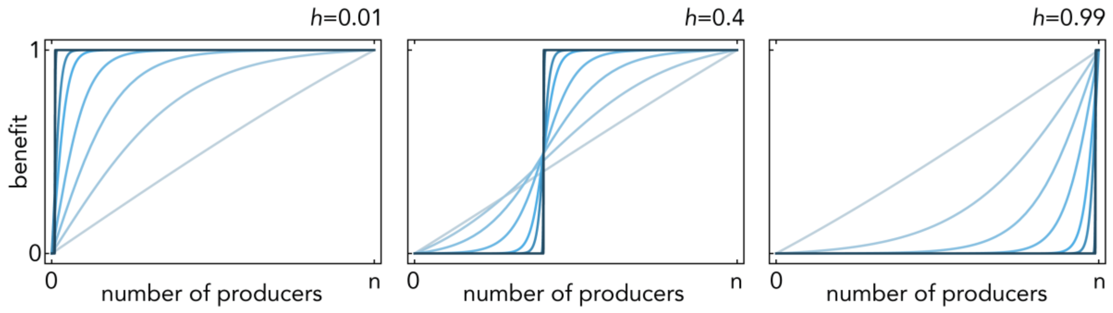
The parameter h defines the position of the inflection point: h→1 gives increasing returns and h→0 diminishing returns; s defines the steepness of the function at the inflection point (s→∞ models a threshold public goods game; s→0 models an NPD; the normalization in (9) in prevents the logistic function (10) from becoming constant for s→0) (Figure 1).
When the benefit b(i) is a nonlinear function such as the one in (9) the roots of in (6) cannot be found analytically. We can, however, characterize the dynamics exactly, and approximate the equilibria, by resorting to the properties of Bernstein polynomials.
2.3. Bernstein Polynomials
Bernstein polynomials were introduced 100 years ago by Sergei Natanovich Bernstein [48] in order to constructively (employing only basic algebra) prove the Weierstrass approximation theorem: given any continuous function f(x) on an interval [a,b] and a tolerance ε > 0, a polynomial P(x) of sufficiently high degree exists, such that |f(x)−P(x)|<ε for all x in [a,b]; in other words, polynomials can uniformly approximate any continuous function over a closed interval. Bernstein polynomials are a significant advance over Taylor polynomials, as they are applicable to any continuous function, whereas the Taylor approximation requires the function to be differentiable. Probably because of their slow convergence, however, Bernstein polynomials were for a long time (and still are) a relatively unknown tool in mathematics. A review of the history of Bernstein polynomials [49] and a full treatment are available [50,51,52]. For our purposes, the following definitions are enough to set the problem.
- The Bernstein polynomial basis of degree n on x in [0, 1] is defined, for i = 0, …, n, by
- A polynomial in Bernstein form of degree n associated with any continuous function fi on [0, 1] is defined for each positive integer n as
- fi is called the Bernstein coefficient
The following properties of Bernstein polynomials are sufficient to characterize the dynamics of our system (see [49] for a complete list of properties, and [50,51,52] for further discussion):
- End-point values: The initial and final values of f and F are the same: F(0) = f0; F(1) = fn.
- Shape preservation: F and f have the same shape (monotonicity, convexity, concavity).
- Variation-diminishing property: The number Z of real roots of F in (0,1)is less than the number S of sign changes of f by an even amount: Z = S − 2j for some integer j greater or equal to 0 and lower than the integer part of n/2 [53] (each root contributes according to its multiplicity).
2.4. Characterizing the Dynamics
Compare (11) with (1) and (12) with (6); in (6) is, by definition, a polynomial in Bernstein form and Δbi is its Bernstein coefficient. Hence, based on the properties defined above, it is straightforward to characterize the dynamics of a nonlinear public goods game based on the number of sign changes of the Bernstein coefficient Δbi instead of inspecting the gradient of selection of the Bernstein polynomial . This Bernstein approach was introduced to study public goods games with sigmoid benefits in the context of cancer biology [39,40]. Games with concave or convex benefits can be analyzed [54] without resorting to the properties of Bernstein polynomials, although in that case the proof is unnecessarily long—the proof is trivial using the Bernstein approach (the results of this exercise have been published in [55], which also replicated the sigmoid case analyzed in [39]).
For games in which the Bernstein coefficient never changes sign, obviously, there is no interior equilibrium. An example of this case is the NPD.
Games with concave or convex benefits are cases in which there can be at most one sign change (Figure 2). If the Bernstein coefficient has one sign change, then there is a unique interior equilibrium x* in (0,1): if the initial sign is +, then x* is stable and x = 0 and x = 1 are unstable: an example of this occurs in games with concave benefits when Δbn−1 < c < Δb0; if the initial sign is -, then x* is unstable and x = 0 and x = 1 are stable: an example of this occurs in games with convex benefits when Δb0 < c < Δbn−1. Games with concave or convex benefits can also have no sign change. Hence, with concave benefits, if c ≥ Δb0 then x = 0 is the unique stable equilibrium and x = 1 is the unique unstable equilibrium; if Δbn−1 < c < Δb0 then there is a unique interior stable equilibrium and x = 0, x = 1 are unstable equilibria; if c ≤ Δbn−1 then x = 1 is the unique stable equilibrium and x = 0 is the unique unstable equilibrium. With convex benefits, if c ≥ Δbn−1 then x = 0 is the unique stable equilibrium and x = 1 is the unique unstable equilibrium; if Δb0 < c < Δbn−1 then there is a unique interior unstable equilibrium and x = 0, x = 1 are stable equilibria; if c ≤ Δb0 then x = 1 is the unique stable equilibrium and x = 0 is the unique unstable equilibrium. In summary, games with concave or convex benefits can have at most one interior equilibrium, either stable or unstable (Figure 2).
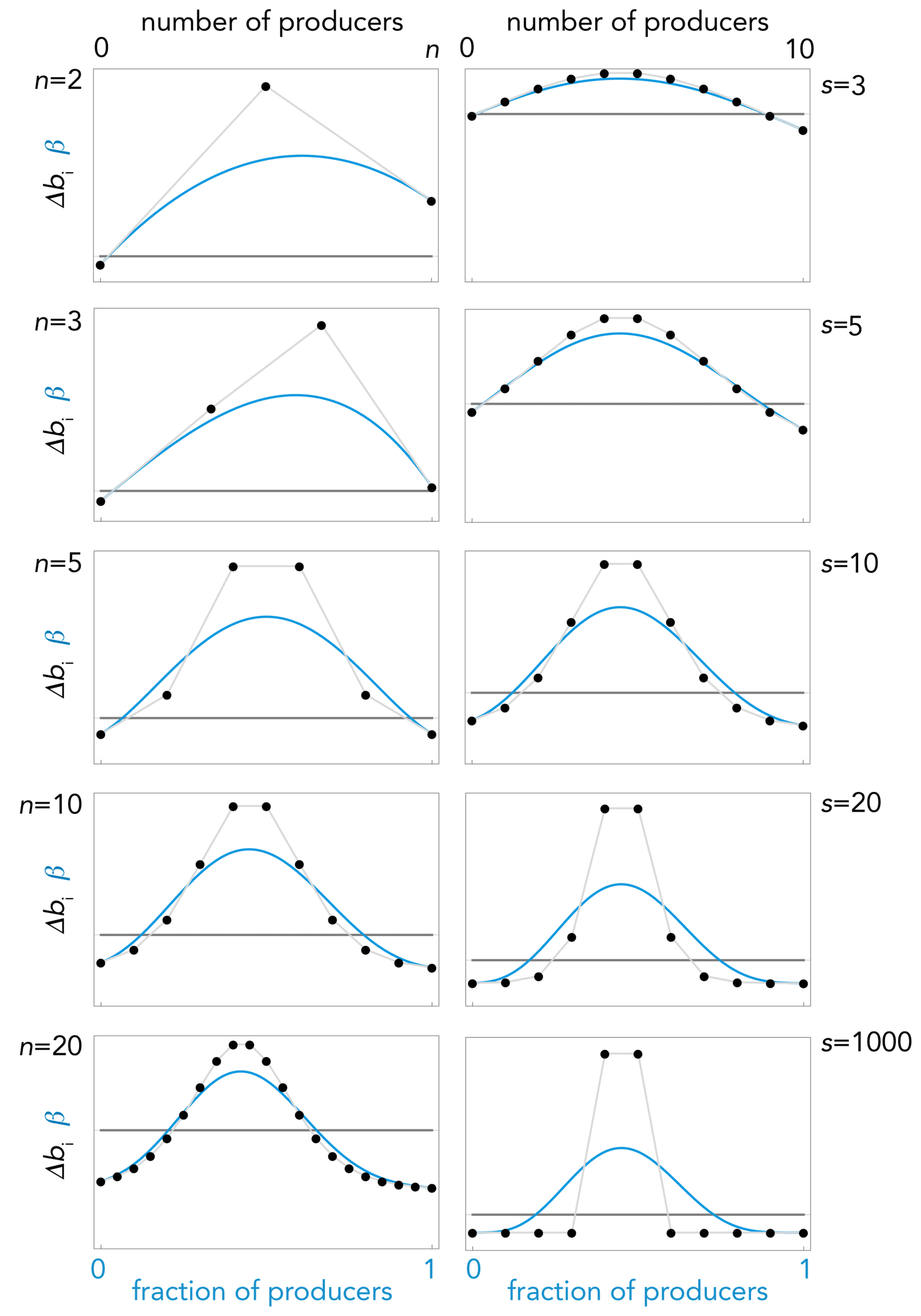
The Bernstein approach is however essential to characterize the dynamics of games with sigmoid benefits [39,40]. If b is sigmoid, that is an h (the inflection point) exists such that Δbi is increasing for i < h, decreasing for i > h, and satisfies Δbi ≠ 0 ∀i, then Δbi is single-peaked and can have at most two sign changes (Figure 3); thus, there are either two interior rest points, or one (if they coincide) or zero, and the dynamics can be characterized as follows:
- If c ≥ (the maximum value of ) there is a unique stable equilibrium x = 0 (producers go extinct) (c1 in Figure 3)
- If Max[Δb0, Δbn−1] ≤ c < there are two stable equilibria: a pure equilibrium x = 0 made of all non-producers and a mixed equilibrium x*; the basins of attraction of these two equilibria are separated by a mixed unstable equilibrium x^; if the initial frequency of producers x < x^ the population will evolve to x = 0; if x > x^ it will evolve to x* (c2 in Figure 3).
- If Δb0 ≤ c < Δbn−1 (this case can exist only for h > 0.5) there is a unique interior unstable equilibrium x^ separating the basins of attraction of two pure stable equilibria: x = 0 and x = 1; if x < x^ the population will evolve to x = 0; if x > x^ it will evolve to x = 1 (c3 in Figure 3).
- If Δbn−1 ≤ c < Δb0 (this case can exist only for h < 0.5) there is a unique interior stable equilibrium x*, to which the population will converge irrespective of the initial frequencies of the two types (c3 in Figure 3).
- If c < Min[Δb0, Δbn−1] there is a unique stable equilibrium x = 1 (non-producers will go extinct) (c4 in Figure 3).
In summary, nonlinear games with collective interactions in which the benefit is a sigmoid function of the frequency of cooperators can have at most two internal equilibria, one of which can be stable (Figure 3).
The dynamics is the same for any benefit function in which Δbi increases for i < h and decreases for i > h. Figure 4 shows two examples of a more complex benefit function, and a case in which the benefits of the two strategies are different functions.
Figure 4A shows the dynamics for the upregulation of glycolysis in cancer cells (the “Warburg effect”)—another example of cooperation for the production of a public good [40] (as it is energetically inefficient under adequate oxygen supply, glycolysis is costly; the products of glycolysis, however, induce the acidification of the microenvironment, which is beneficial to all cancer cells, irrespective of their metabolism). To take into account the possibility that high levels of glycolysis are detrimental to tumor cells (self-poisoning) we must use a double sigmoid function, monotonically increasing for i < d and monotonically decreasing for i > d:
where
The parameter d describes the value of i at which the benefits of acidity are overcome by the deleterious effects of self-poisoning; for i < dn, the function is monotonically increasing and has an inflection point at h1 and steepness s1; for i > dn, the function is monotonically decreasing and has an inflection point at h2 and steepness s2 (with 0 < h1, h2 ≤ 1 and s1,s2 > 0); the additional parameter y measures the maximum damage of self-poisoning. While analyzing the gradient of selection with benefits given by (13) appears hopeless, the Bernstein approach enables us to characterize the dynamics simply by looking at the number and type of sign changes of the Bernstein coefficient, as shown in Figure 4A.
Figure 4B shows another class of games that appear analytically unsolvable but that are easily characterized using the Bernstein approach. In tumor-stroma interactions, the fitness of cancer cells is an increasing function of the fraction of stromal cells, while the fitness of stromal cells is an increasing function of the fraction of cancer cells (because of stroma and tumor exchange growth factors that are mutually beneficial). Figure 4B shows the simplest model of this scenario with benefit functions for the tumor and stroma increasing in opposite directions, that is, given by:
2.5. Comparison with Pairwise and Linear Games
Let us consider again the case of sigmoid benefits. Note how the steepness of the benefit function affects the dynamics (Figure 5): as we have seen, games with linear benefits (s→0) have no interior equilibria; as steepness increases interior equilibria, stable and (or) unstable, arise; also note that the approximation of the gradient of selection to its Bernstein coefficient is less accurate as s increases, and becomes inaccurate when the sigmoid function approaches a step function (s→∞).
Figure 5 also shows an example of the difference between games with pairwise interactions and collective interactions. Two-player games are a special case of collective games with n = 2 and thus there are only one or zero sign changes; not surprisingly, therefore, there are only four possible types of sign change (always +; always −; from + to −; from − to +) and therefore four possible types of dynamics and four types of equilibria in games with two strategies with pairwise interactions (the same types we saw for concave and convex benefits).
2.6. Finding the Equilibria
We can find the internal equilibria analytically by setting to zero, instead of the gradient of selection, its Bernstein coefficient Δbi, resorting to an additional property of Bernstein polynomials–Bernstein theorem: A Bernstein polynomial F(x) converges uniformly to its coefficient f(x) in [0, 1], that is, . The approximation is rather slow. By Voronovskaya’s theorem [56], for functions that are twice differentiable:
In our case, let us call the benefit for having a fraction x of producers b(x) = 1/[1 + es(h−x)], the extension of b(i) in (9) to all x [0, 1], with x = i/n. Let us first consider the non-normalized version in (10), that is, let us assume that b(i) = l(i);
is a Bernstein polynomial of the coefficient Δb = b((i + 1)/n) − b(i/n), and by Bernstein theorem we know that it converges uniformly to Δb in [0, 1]. Furthermore, because Δb is the forward difference of the benefit function with spacing 1/n, for large enough n we can approximate Δb using the derivative of the benefit function, that is Δb ≅ (1/n)b’(i/n). For any given x, i/n converges in probability to x as n→∞, therefore by Bernstein theorem converges to (1/n)b’(x), and we can find the equilibria by setting , which yields:
b’(x) = cn
Using this approach [39], the equilibrium frequencies can be found by
provided that c > Min[Δb0, Δbn−1] (otherwise x = 1 is the only stable equilibrium) and c < s/4n (otherwise x = 0 is the only stable equilibrium). A qualitatively equivalent result holds for the normalized version in (9), because b(i) differs from l(i) only by the inclusion of the normalizing term. For the normalized version, the equilibria are given by
where B = b(1) − b(0).
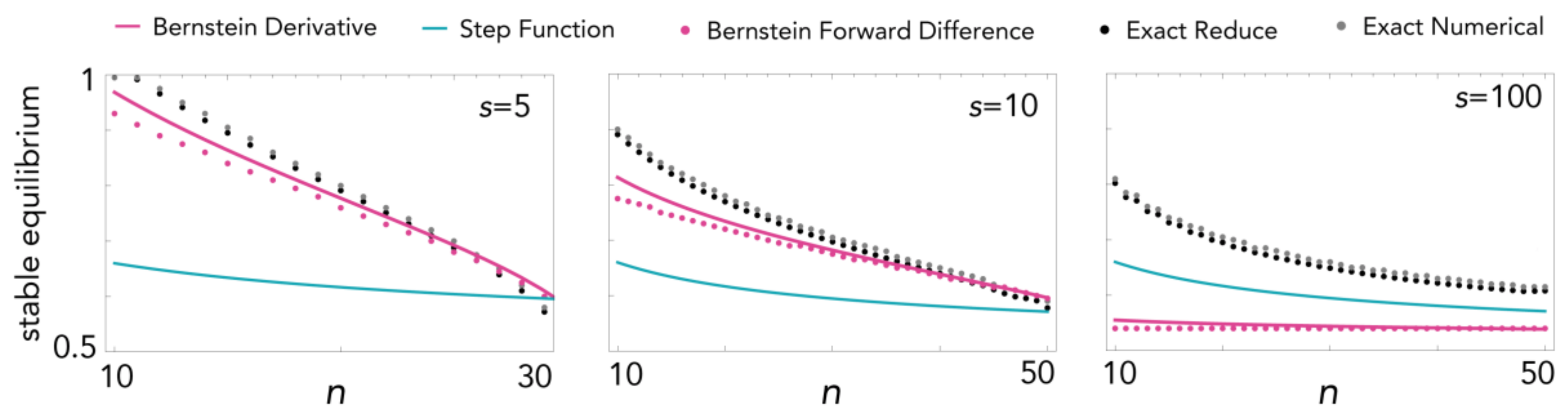
2.7. Goodness of the Approximation
The error of the approximation Δb − is shown in Figure 6: convergence is slower as nonlinearity (s) increases (as we know from Voronovskaya’s theorem); it improves with n (an obvious consequence of Bernstein theorem) and as the equilibrium gets close to 1 or 0 (from the end-point values property of the Bernstein polynomials).
2.8. Approaches to Calculate the Equilibria
In practice the best approach to calculate the equilibria depends mainly on n and s:
- Using the exact formula from (8), by setting (x) = 0. This is a reasonable approach for n not too large (the “Reduce” command in Mathematica 11, on a laptop with a 2.9 GHz processor and 16 GB of memory, enables this for n up to about 50) but the results become inaccurate as n grows and it is hopeless for very large n, when numerical methods become necessary.
- The equilibrium can also be approximated by setting Δb = 0, but similar computational problems arise.
- Using the Bernstein approximation outlined above, the equilibrium can be easily calculated for any n from Equations (21)–(24). The accuracy of this approach, as we have seen (Figure 6), improves with n and declines with s.
- For large n and large s, an alternative method is to find the equilibria of a Heaviside step function with the same inflection h using the following equation (25) (where k = hn):
For steep sigmoid functions, the approximation to a step function is more precise than the Bernstein approximation (Figure 7) (It is perhaps of some mathematical interest to note that the envelope of the Bernstein polynomial basis of degree n is [57], which coincides with the Stirling approximation of the ith Bernstein polynomial basis of degree n on i/n at equilibrium for threshold public goods games [35]).
2.9. More Than Two Strategies
The analysis remains problematic for games with more than two strategies. Nonlinearities, however, are clearly still important. Let us examine a game with three strategies with the following payoffs (another case of tumor-stroma interactions, similar to the example described above, but with an additional type with constant fitness γ):
where j is the number of players of type C in the group (of size n) and
where the parameters h1 and h2 are analogous to h and the parameters s1 and s2 are analogous to s, thus (32) and (33) are sigmoid functions that can range from linear to step functions. In an infinite well-mixed population, if xC is the frequency of cells of type C, the fitness of the three types are:
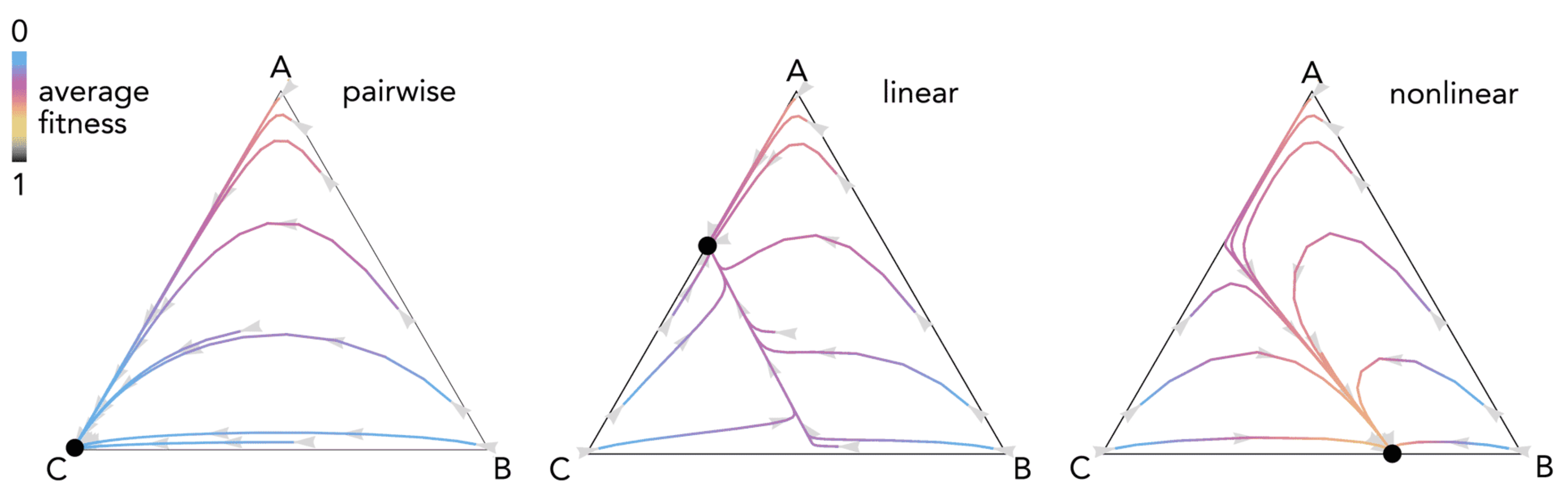
that is, type A has constant fitness; the fitness of type B increases with the number of players of type C; the fitness of type C increases with the number of players of type B. Figure 8 shows an example of the differences between pairwise, linear, and nonlinear models.
ωA = γ
ωB(j) = r[LB(j) − LB(0)]/[LB(n) − LB(0)]
ωC(j) = 1 − [LC(j) − LC(0)]/[LC(n) − LC(0)]
3. Conclusions
Pairwise games and games with collective interactions can have different dynamics and equilibria [31,32]. As we have seen here, nonlinearities also have profound effects; the main difference is that pairwise and linear games usually lack the internal equilibria that are often observed in nonlinear games. This means that if benefits are nonlinear, a stable coexistence of cooperators and free-riders is often possible without positive assortment or incentives. This is in direct contradiction with most of the theoretical models that have been developed in biology—which are based on the assumption of linear benefits or pairwise games, and therefore require positive assortment between cooperators (brought about by genetic relatedness [58,59], spatial structure [60] or repeated interactions [61]) to maintain cooperation. As we have seen, with nonlinear benefits cooperation can persist as a mixture of producers and non-producers because of the nonlinear effects of the interactions.
In models of game theory of cancer with two strategies, nonlinear effects help explain seemingly puzzling empirical observations such as the persistence of intra-tumor heterogeneity and the Warburg effect [37,38,39,40,41,42,43,44]. Three-strategy games have been used to model tumor-stroma interactions in multiple myeloma and have also shown that assuming pairwise interactions [27] leads to results that differ significantly from a model with collective interactions [46], with implications for disease progression and treatment. Extending the same model to a game with nonlinear benefits reveals further differences [Sartakhti, et al., this issue].
Neglecting collective interactions and nonlinearities can also lead to other more subtle but equally misleading errors. For instance, invertase production in yeast, a clear example of diffusible public good, has been modelled as a game with pairwise interactions, initially as a PD [62] and eventually as a game of Chicken [63] leading to an incorrect prediction that still persist in microbiology: maximum growth in experimental populations of microbes is often observed at intermediate frequencies of cooperators—a fact that is often highlighted as puzzling [64] because it is based on predictions for pairwise game or linear benefits, which predicts maximum cooperation when the cooperators go to fixation; in multiplayer nonlinear games, however, it is not surprising that maximum fitness occurs for intermediate frequencies of cooperators [32].
Neglecting nonlinearities in public goods games can lead to crucial mistakes in the basic results and fundamental misunderstanding. The approach described here offers a relatively simple way to study games with payoffs that are seemingly impossible to analyze. Even for more complex cases in which the Bernstein approach fails, we should nonetheless insist on using nonlinear public goods games.
Acknowledgments
This project has received funding from the Marie Curie International Outgoing Fellowship within the 7th European Community Framework Program under grant agreement No 627816-dunharrow.
Conflicts of Interest
The author declares no conflict of interest.
References
- Hardin, J. The tragedy of the commons. Science 1968, 162, 1243–1248. [Google Scholar] [CrossRef] [PubMed]
- Burt, A.; Trivers, R. Genes in Conflict; Harvard University Press: Cambridge, MA, USA, 2006. [Google Scholar]
- West, S.A.; Diggle, S.P.; Buckling, A.; Gardner, A.; Griffin, A.S. The social lives of microbes. Annu. Rev. Ecol. Evol. Syst. 2007, 38, 53–77. [Google Scholar] [CrossRef]
- Jouanneau, J.; Moens, G.; Bourgeois, Y.; Poupon, M.F.; Thiery, J.P. A minority of carcinoma cells producing acidic fibroblast growth factor induces a community effect for tumor progression. Proc. Nat. Acad. Sci. USA 1994, 91, 286–290. [Google Scholar] [CrossRef] [PubMed]
- Axelrod, R.; Axelrod, D.E.; Pienta, K.J. Evolution of cooperation among tumor cells. Proc. Nat. Acad. Sci. USA 2006, 103, 13474–13479. [Google Scholar] [CrossRef] [PubMed]
- Packer, C.; Scheel, D.; Pusey, A.E. Why lions form groups, food is not enough. Am. Nat. 1990, 136, 1–19. [Google Scholar] [CrossRef]
- Maynard Smith, J.; Szathmáry, E. The Major Transitions in Evolution; Freeman: San Francisco, CA, USA, 1995. [Google Scholar]
- Tucker, A. A two-person dilemma (1950). In Readings in Games and Information; Rasmusen, E., Ed.; Blackwell: Oxford, UK, 2001; pp. 7–8. [Google Scholar]
- Rapoport, A.; Chammah, A.M. The game of chicken. Am. Behav. Sci. 1966, 10, 10–28. [Google Scholar] [CrossRef]
- Maynard Smith, J.; Price, G.R. The logic of animal conflict. Nature 1973, 246, 15–18. [Google Scholar] [CrossRef]
- Sugden, R. The Economics of Rights, Cooperation and Welfare; Blackwell: Oxford, UK, 1986. [Google Scholar]
- Hamburger, H. N-person Prisoners Dilemma. J. Math. Sociol. 1973, 3, 27–48. [Google Scholar] [CrossRef]
- Fox, J.; Guyer, M. Public Choice and cooperation in N-person Prisoner’s Dilemma. J. Confl. Resolut. 1978, 22, 469–481. [Google Scholar] [CrossRef]
- Rankin, D.J.; Bargum, K.; Kokko, H. The tragedy of the commons in evolutionary biology. Trends Ecol. Evol. 2007, 12, 643–651. [Google Scholar] [CrossRef] [PubMed] [Green Version]
- Kollock, P. Social dilemmas, the anatomy of cooperation. Ann. Rev. Sociol. 1998, 24, 183–214. [Google Scholar] [CrossRef]
- Cornish-Bowden, A. Fundamentals of Enzyme Kinetics, 4th ed.; Wiley Blackwell: Hoboken, NJ, USA, 2012. [Google Scholar]
- Frank, S.A. Input-output relations in biological systems, measurement, information and the Hill equation. Biol. Dir. 2013, 8, 31. [Google Scholar] [CrossRef] [PubMed]
- Archetti, M.; Scheuring, I. Evolution of optimal Hill coefficients in nonlinear public goods games. J. Theor. Biol. 2016, 406, 73–82. [Google Scholar] [CrossRef] [PubMed] [Green Version]
- Tomlinson, I.P. Game-theory models of interactions between tumour cells. Eur. J. Cancer 1997, 33, 1495–1500. [Google Scholar] [CrossRef]
- Tomlinson, I.P.; Bodmer, W.F. Modelling consequences of interactions between tumour cells. Br. J. Cancer 1997, 75, 157–160. [Google Scholar] [CrossRef] [PubMed]
- Bach, L.A.; Bentzen, S.; Alsner, J.; Christiansen, F.B. An evolutionary-game model of tumour cell interactions, possible relevance to gene therapy. Eur. J. Cancer 2001, 37, 2116–2120. [Google Scholar] [CrossRef]
- Bach, L.A.; Sumpter, D.J.T.; Alsner, J.; Loeschke, V. Spatial evolutionary games of interaction among generic cancer cells. J. Theor. Med. 2003, 5, 47–58. [Google Scholar] [CrossRef]
- Basanta, D.; Hatzikirou, H.; Deutsch, A. Studying the emergence of invasiveness in tumours using game theory. Eur. Phys. J. 2008, 63, 393–397. [Google Scholar] [CrossRef]
- Basanta, D.; Simon, M.; Hatzikirou, H.; Deutsch, A. Evolutionary game theory elucidates the role of glycolysis in glioma progression and invasion. Cell Prolif. 2008, 41, 980–987. [Google Scholar] [CrossRef] [PubMed]
- Basanta, D.; Scott, J.G.; Rockne, R.; Swanson, K.R.; Anderson, A.R. The role of IDH1 mutated tumour cells in secondary glioblastomas, an evolutionary game theoretical view. Phys. Biol. 2011, 8, 015016. [Google Scholar] [CrossRef] [PubMed]
- Basanta, D.; Scott, J.G.; Fishman, M.N.; Ayala, G.; Hayward, S.W.; Anderson, A.R. Investigating prostate cancer tumour-stroma interactions, clinical and biological insights from an evolutionary game. Br. J. Cancer 2012, 106, 174–181. [Google Scholar] [CrossRef] [PubMed] [Green Version]
- Dingli, D.; Chalub, F.A.; Santos, F.C.; Pacheco, J. Cancer phenotype as the outcome of an evolutionary game between normal and malignant cells. Br. J. Cancer 2009, 101, 1130–1136. [Google Scholar] [CrossRef] [PubMed]
- Gerstung, M.; Nakhoul, H.; Beerenwinkel, N. Evolutionary games with affine fitness functions, applications to cancer. Dyn. Games Appl. 2011, 1, 370–385. [Google Scholar] [CrossRef]
- You, L.; Brown, J.S.; Thuijsman, F.; Cunningham, J.J.; Gatenby, R.A.; Zhang, J.S.; Stankova, K. Spatial vs. non-spatial eco-evolutionary dynamics in a tumor growth model. J. Theor. Biol. 2017, 435, 78–97. [Google Scholar] [CrossRef] [PubMed]
- Zhang, J.S.; Cunningham, J.J.; Brown, J.S.; Gatenby, R.A. Integrating evolutionary dynamics into treatment of metastatic castrate-resistant prostate cancer. Nat. Commun. 2017, 8, 1816. [Google Scholar] [CrossRef] [PubMed]
- Broom, M.; Cannings, C.; Vickers, G.T. Multiplayer matrix games. Bull. Math. Biol. 1997, 59, 931–952. [Google Scholar] [CrossRef] [PubMed]
- Archetti, M.; Scheuring, I. Review: Game theory of public goods in one-shot social dilemmas without assortment. J. Theor. Biol. 2012, 299, 9–20. [Google Scholar] [CrossRef] [PubMed]
- Archetti, M. The volunteer’s dilemma and the optimal size of a social group. J. Theor. Biol. 2009, 261, 475–480. [Google Scholar] [CrossRef] [PubMed]
- Archetti, M. Cooperation as a volunteer’s dilemma and the strategy of conflict in public goods games. J. Evol. Biol. 2009, 22, 2192–2200. [Google Scholar] [CrossRef] [PubMed]
- Archetti, M.; Scheuring, I. Coexistence of cooperation and defection in public goods games. Evolution 2011, 65, 1140–1148. [Google Scholar] [CrossRef] [PubMed]
- Boza, G.; Számadó, S. Beneficial laggards, multilevel selection, cooperative polymorphism and division of labour in threshold public good games. BMC Evol. Biol. 2010, 10, 336. [Google Scholar] [CrossRef] [PubMed]
- Archetti, M. Dynamics of growth factor production in monolayers of cancer cells. Evol. Appl. 2013, 6, 1146–1159. [Google Scholar] [CrossRef] [PubMed] [Green Version]
- Archetti, M. Evolutionarily stable anti-cancer therapies by autologous cell defection. Evol. Med. Public Health 2013, 1, 161–172. [Google Scholar] [CrossRef] [PubMed]
- Archetti, M. Evolutionary game theory of growth factor production, implications for tumor heterogeneity and resistance to therapies. Br. J. Cancer 2013, 109, 1056–1062. [Google Scholar] [CrossRef] [PubMed] [Green Version]
- Archetti, M. Evolutionary dynamics of the Warburg effect, glycolysis as a collective action problem among cancer cells. J. Theor. Biol. 2014, 341, 1–8. [Google Scholar] [CrossRef] [PubMed] [Green Version]
- Archetti, M. Stable heterogeneity for the production of diffusible factors in cell populations. PLoS ONE 2014, 9, e108526. [Google Scholar] [CrossRef] [PubMed] [Green Version]
- Archetti, M. Heterogeneity and proliferation of invasive cancer subclones in game theory models of the Warburg effect. Cell Prolif. 2015, 482, 259–269. [Google Scholar] [CrossRef] [PubMed] [Green Version]
- Archetti, M. Cooperation among cancer cells as public goods games on Voronoi networks. J. Theor. Biol. 2016, 396, 191–203. [Google Scholar] [CrossRef] [PubMed] [Green Version]
- Archetti, M.; Ferraro, D.A.; Christofori, G. Heterogeneity for IGF-II production maintained by public goods dynamics in neuroendocrine pancreatic cancer. Proc. Nat. Acad. Sci. USA 2015, 112, 1833–1838. [Google Scholar] [CrossRef] [PubMed] [Green Version]
- Kaznatcheev, A.; Velde, R.V.; Scott, J.G.; Basanta, D. Cancer treatment scheduling and dynamic heterogeneity in social dilemmas of tumour acidity and vasculature. Br. J. Cancer 2018, in press. [Google Scholar]
- Sartakhti, J.S.; Manshaei, M.H.; Bateni, S.; Archetti, M. Evolutionary dynamics of tumor-stroma interactions in multiple myeloma. PLoS ONE 2016, 1112, e0168856. [Google Scholar] [CrossRef] [PubMed]
- Hofbauer, J.; Sigmund, K. Evolutionary Games and Population Dynamics; Cambridge University Press: Cambridge, UK, 1998. [Google Scholar]
- Bernstein, S. Démonstration du théorème de Weierstrass fondée sur le calcul des probabilities. Comm. Soc. Math. Kharkov 1912, 13, 1–2. [Google Scholar]
- Farouki, R.T. The Bernstein polynomial basis, a centennial retrospective. Comput. Aided Geom. Des. 2012, 29, 379–419. [Google Scholar] [CrossRef]
- Lorentz, G.G. Bernstein Polynomials; University of Toronto Press: Toronto, ON, Canada, 1953. [Google Scholar]
- DeVore, R.A.; Lorentz, G.G. Constructive Approximation; Springer: Berlin, Germany, 1993. [Google Scholar]
- Phillips, G.M. Interpolation and Approximation by Polynomials; Springer: Berlin, Germany, 2003. [Google Scholar]
- Schoenberg, I.J. On variation diminishing approximation methods. In On Numerical Approximation; Langer, R.E., Ed.; University of Wisconsin Press: Madison, WI, USA, 1959. [Google Scholar]
- Motro, U. Cooperation and defection, playing the field and the ESS. J. Theor. Biol. 1991, 151, 145–154. [Google Scholar] [CrossRef]
- Pena, G.; Lehmann, L.; Noeldeke, G. Gains from switching and evolutionary stability in multi-player matrix games. J. Theor. Biol. 2014, 346, 23–33. [Google Scholar] [CrossRef] [PubMed] [Green Version]
- Voronovskaya, E. Détermination de la forme asymptotique d’ approximation des fonctions par les polynômes de M. Bernstein. CR Acad. Sci. URSS 1932, 79, 79–85. [Google Scholar]
- Mabry, R. Problem 10990. Am. Math. Mon. 2003, 110, 59. [Google Scholar] [CrossRef]
- Hamilton, W.D. The genetical evolution of social behaviour. J. Theor. Biol. 1964, 7, 1–52. [Google Scholar] [CrossRef]
- Frank, S.A. Foundations of Social Evolution; Princeton University Press: Princeton, NJ, USA, 1998. [Google Scholar]
- Nowak, M.A. Evolutionary Dynamics; Harvard University Press: Cambridge, MA, USA, 2006. [Google Scholar]
- Axelrod, R.; Hamilton, W.D. The Evolution of cooperation. Science 1981, 211, 1390–1396. [Google Scholar] [CrossRef] [PubMed]
- Greig, D.; Travisano, M. The Prisoner’s Dilemma and polymorphism in yeast SUC genes. Proc. R. Soc. Lond. Ser. B 2004, 27, S25–S26. [Google Scholar] [CrossRef] [PubMed]
- Gore, J.; Youk, H.; van Oudenaarden, A. Snowdrift game dynamics and facultative cheating in yeast. Nature 2009, 459, 253–256. [Google Scholar] [CrossRef] [PubMed]
- MacLean, R.C.; Fuentes-Hernandez, A.; Greig, D.; Hurst, L.D.; Gudelj, I. A Mixture of “Cheats” and “Co-Operators” Can Enable Maximal Group Benefit. PLoS Biol. 2010, 8, e1000486. [Google Scholar] [CrossRef] [PubMed]
Figure 1.
Sigmoid benefits. The benefit b(i) of a public good as a function of the number of producers (i), described by a normalized logistic function (Equation (9)) with inflection point h; h→1 gives increasing returns and h→0 diminishing returns. Multiple curves are shown, with increasing steepness s (increasing opacity).

Figure 2.
The gradient of selection (bottom panels, continuous blue line) and its Bernstein coefficient Δbi (bottom panels, dotted line) for different types of benefit functions (top panels): concave (n = 9, h = 0.1, s = 10, c = 0.1); convex (n = 9, h = 0.9, s = 10, c = 0.1); sigmoid (n = 10, h = 0.4, s = 9, c = 0.1); step function (n = 9, h = 0.4, s = 1000, c = 0.1). Arrows show the direction of the dynamics (determined by the sign of the gradient of selection); squares show the equilibria (full: stable; empty: unstable).
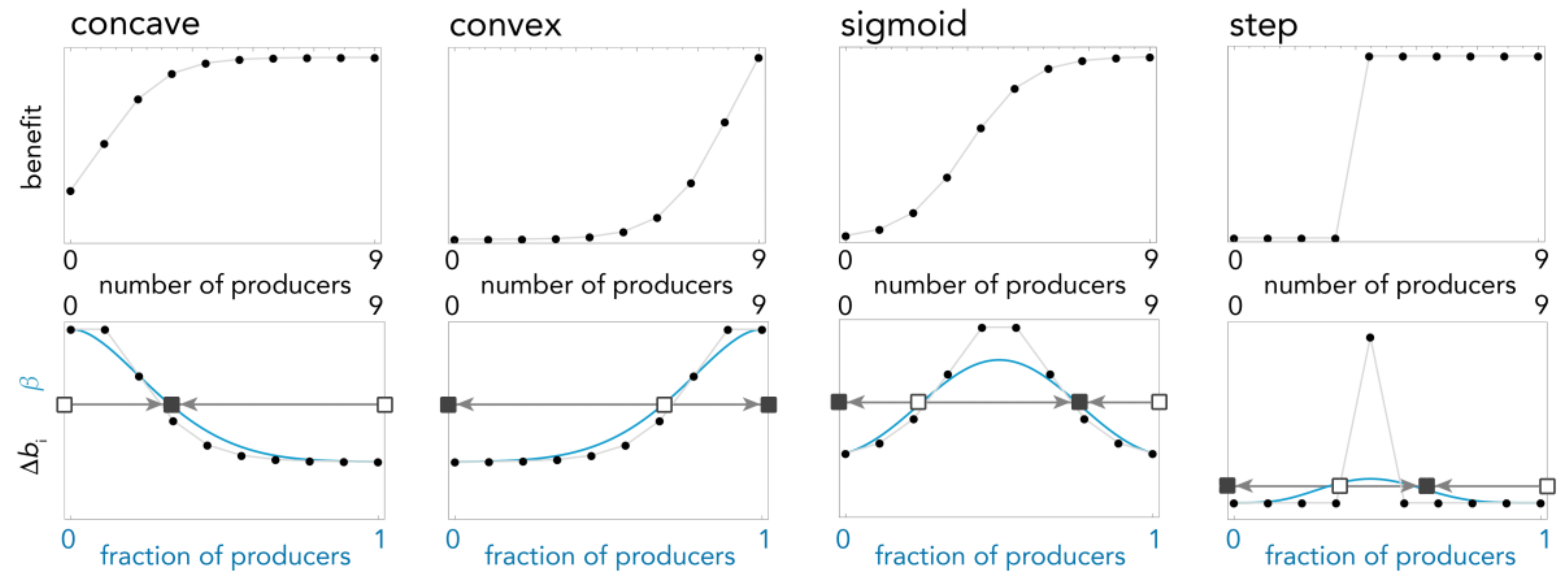
Figure 3.
Types of dynamics when the benefit is a sigmoid function. The gradient of selection (continuous blue line) and its Bernstein coefficient Δbi (dotted line); squares show the equilibria (full: stable; empty: unstable) for different values of c (gray lines); arrows show the direction of the dynamics (determined by the sign of the gradient of selection); s = 5; n = 9, h = 0.4 or 0.6.
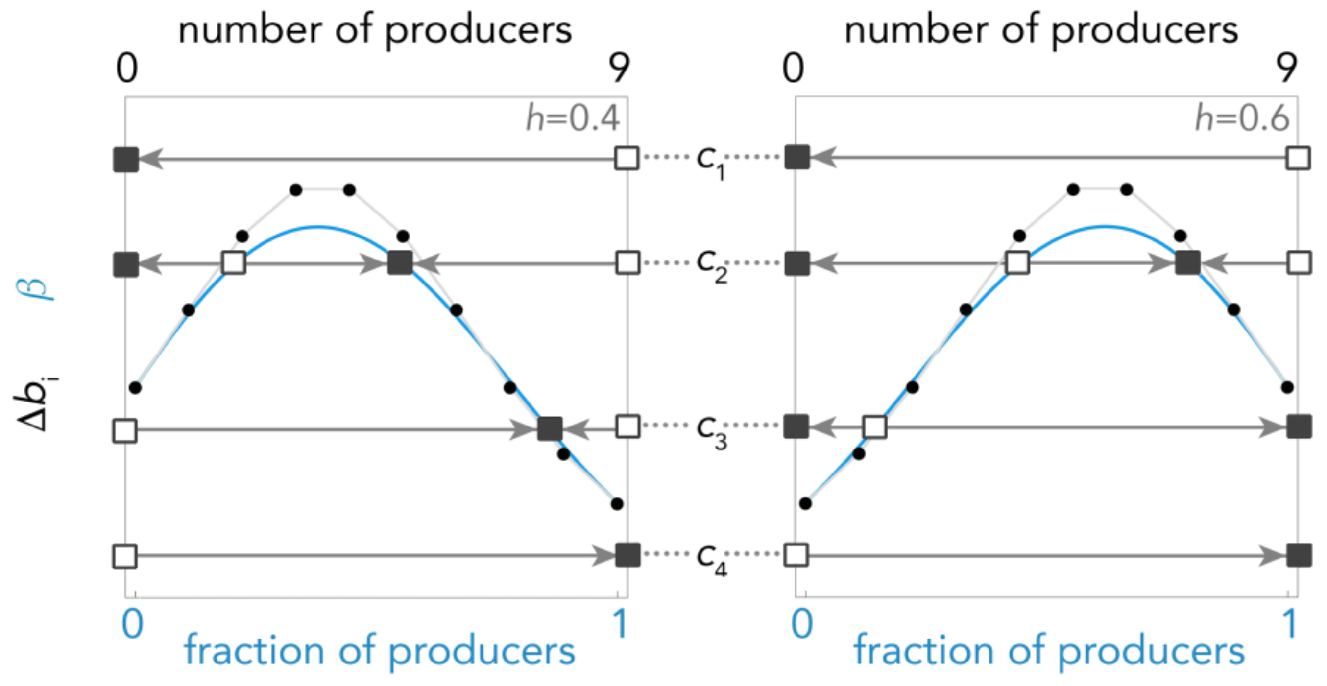
Figure 4.
The gradient of selection (continuous blue line) and its Bernstein coefficient Δbi (dotted line) for more complex functions; squares show the equilibria (full: stable; empty: unstable); arrows show the direction of the dynamics (determined by the sign of the gradient of selection); A: The double inverse sigmoid function described in (13) (n = 10, h1 = 0.4, h2 = 0.2, s1 = 10, s2 = 10, c = 0.1, y = 2, d = 0.5). B: Two different benefit functions described by (16) and (17) (n = 10, h1 = 0.6, h2 = 0.2, s1 = 5, s2 = 20, c = 0.1).
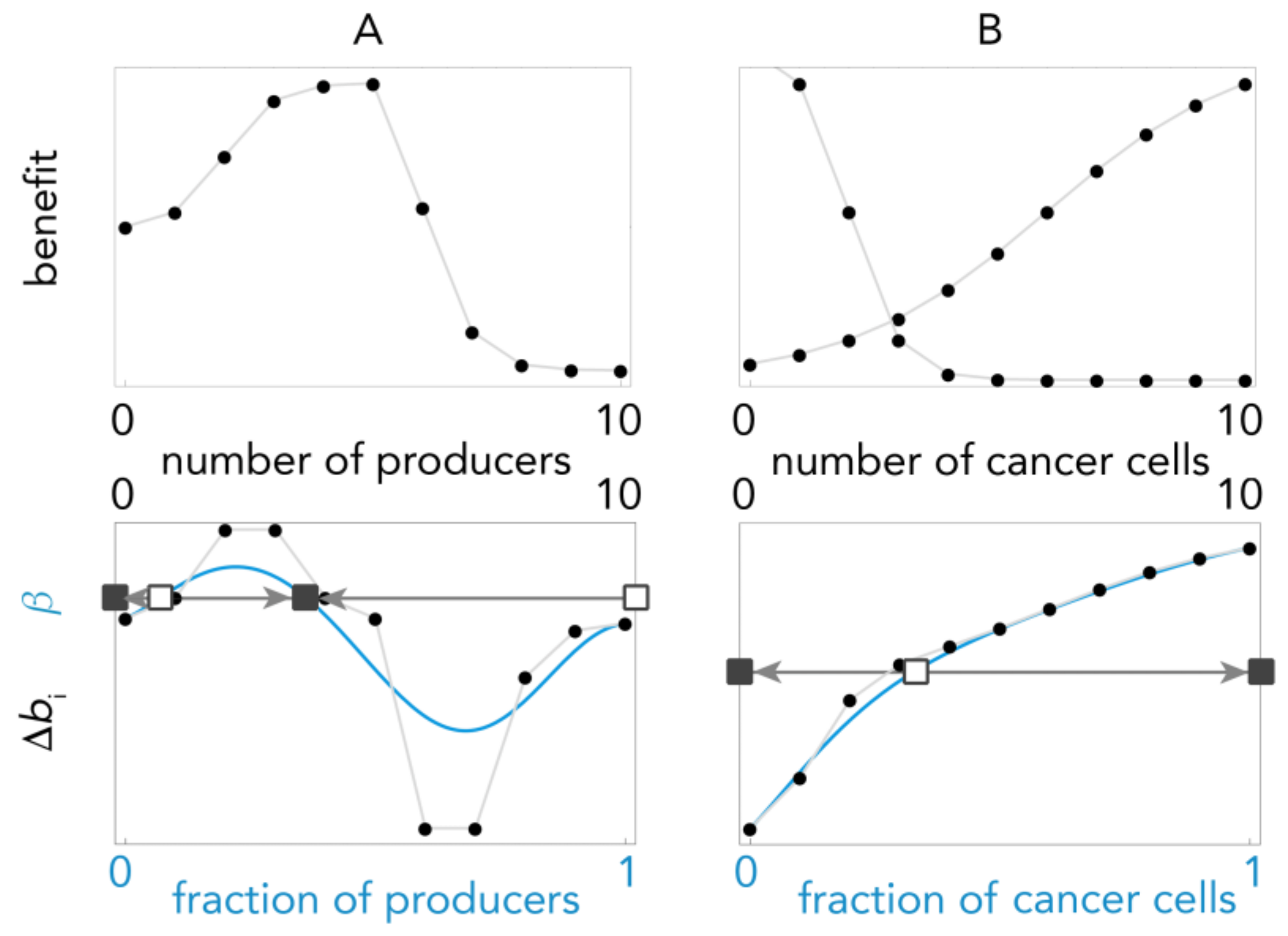
Figure 5.
Effect of s and n. The gradient of selection (continuous blue line) and its Bernstein coefficient Δbi (dotted line) in public goods games with sigmoid benefits, for different values of s (n = 10, h = 0.4, c = 0.05) or for different values of n (s = 10, h = 0.4, c = 0.05); squares show the equilibria (full: stable; empty: unstable); arrows show the direction of the dynamics (determined by the sign of the gradient of selection).

Figure 6.
Error [Δb − ] at the stable equilibrium, as a function of s, for different values of n; c = 0.01, h = 0.5.
Figure 6.
Error [Δb − ] at the stable equilibrium, as a function of s, for different values of n; c = 0.01, h = 0.5.
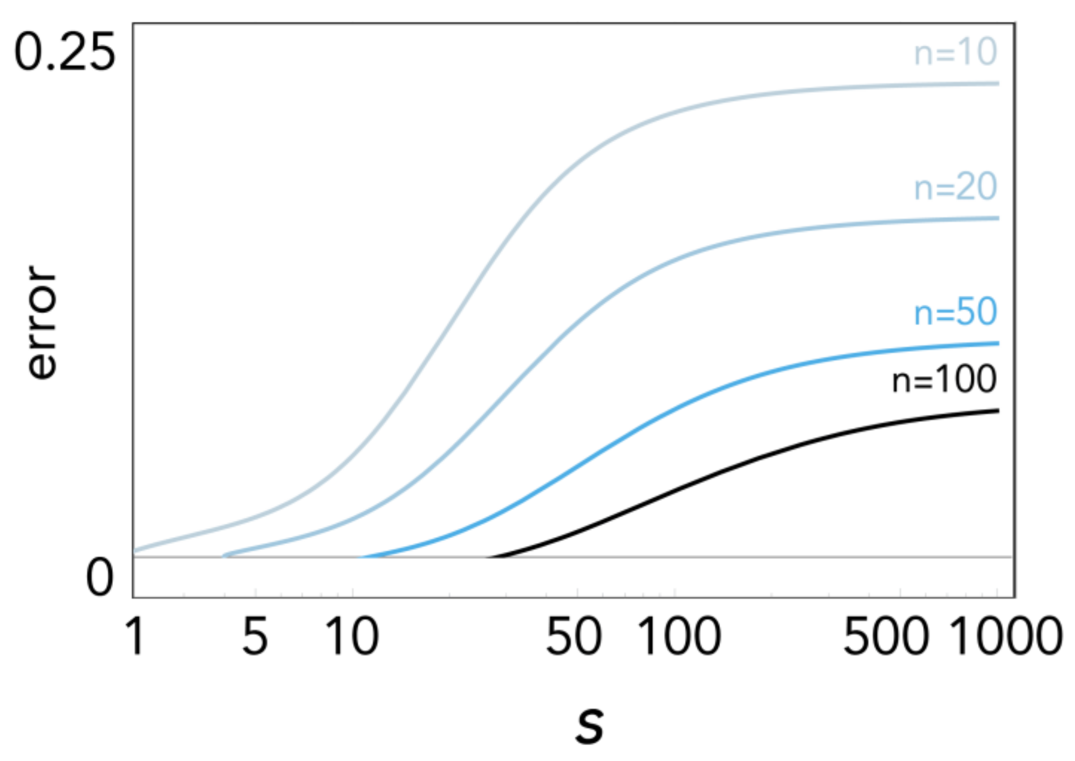
Figure 7.
Comparison between the values of the stable equilibria (as a function of n) calculated using different methods, with c = 0.04, h = 0.5 and different values of s.
Figure 7.
Comparison between the values of the stable equilibria (as a function of n) calculated using different methods, with c = 0.04, h = 0.5 and different values of s.

Figure 8.
Three-strategy game. The dynamics of the three strategies A, B, and C with fitness given by Equations (33)–(35) with n = 20, h1 = 0.2, h2 = 0.4, r = 0.5 with pairwise interactions, linear benefits (s1 = s2 = 0.01) or nonlinear benefits (s1 = 50, s2 = 20).
Figure 8.
Three-strategy game. The dynamics of the three strategies A, B, and C with fitness given by Equations (33)–(35) with n = 20, h1 = 0.2, h2 = 0.4, r = 0.5 with pairwise interactions, linear benefits (s1 = s2 = 0.01) or nonlinear benefits (s1 = 50, s2 = 20).

© 2018 by the authors. Licensee MDPI, Basel, Switzerland. This article is an open access article distributed under the terms and conditions of the Creative Commons Attribution (CC BY) license (http://creativecommons.org/licenses/by/4.0/).
Share and Cite
MDPI and ACS Style
Archetti, M. How to Analyze Models of Nonlinear Public Goods. Games 2018, 9, 17. https://doi.org/10.3390/g9020017
AMA Style
Archetti M. How to Analyze Models of Nonlinear Public Goods. Games. 2018; 9(2):17. https://doi.org/10.3390/g9020017
Chicago/Turabian StyleArchetti, Marco. 2018. "How to Analyze Models of Nonlinear Public Goods" Games 9, no. 2: 17. https://doi.org/10.3390/g9020017
Note that from the first issue of 2016, this journal uses article numbers instead of page numbers. See further details here.